SPRA420A - February 2000
Switched Reluctance Motor Control – Basic Operation and
Example Using the TMS320F240
Michael T. DiRenzo
Digital Signal Processing Solutions
ABSTRACT
This report describes the basic operation of switched reluctance motors (SRMs) and
demonstrates how a TMS320F240 DSP-based SRM drive from Texas Instruments (TI
) can
be used to achieve a wide variety of control objectives.
The first part of the report offers a detailed review of the operation and characteristics of
SRMs. The advantages and disadvantages of this type of motor are cited.
The second part of the report provides an example application of a four-quadrant, variable
speed SRM drive system using a shaft position sensor. The example has complete hardware
and software details for developing an SRM drive system using the TMS320F240. The SRM
operation is described, along with the theoretical basis for designing the various control
algorithms. The example can be used as a baseline design which can be easily modified to
accommodate a specific application.
This report contains material previously released in the Texas Instruments application report
Developing an SRM Drive System Using the TMS320F240 (literature number SPRA420),
and has been updated for inclusion in the Application Design Kit (ADK) for switched
reluctance motors.
Contents
1
Introduction
. . .
2
2
Motor Characteristics
. . .
3
2.1 Torque-Speed Characteristics
. . .
4
2.2 Electromagnetic Equations
. . .
5
2.3 General Torque Equation
. . .
6
2.4 Simplified Torque Equation
. . .
8
3
Control
. . .
9
4
Example – SRM Drive with Position Feedback
. . .
12
4.1 Hardware Description
. . .
12
4.1.1
SRM Characteristics
. . .
12
4.1.2
Control Hardware
. . .
12
4.1.3
Position Sensor
. . .
12
4.1.4
Power Electronics Hardware
. . .
14
4.2 Software Description
. . .
16
4.2.1
Program Structure
. . .
17
4.2.2
Initialization Routines
. . .
20
4.2.3
Current Controller
. . .
21
4.2.4
Position Estimation
. . .
23
4.2.5
Velocity Estimation
. . .
24
4.2.6
Commutation
. . .
27
4.2.7
Velocity Controller
. . .
29
5
References
. . .
32
Appendix A
Software Listings for a TMS320F240-Based SRM Drive With Position Sensor
. . .
34
List of Figures
Figure 1. Various SRM Geometries
. . .
4
Figure 2. SRM Torque-Speed Characteristics
. . .
5
Figure 3. Graphical Interpretation of Magnetic Field Energy
. . .
7
Figure 4. Graphical Interpretation of Magnetic Field Co-Energy
. . .
7
Figure 5. Basic Operation of a Current-Controlled SRM – Motoring at Low Speed
. . .
9
Figure 6. Commutation of a 3-Phase SRM
. . .
10
Figure 7. Single-Pulse Mode – Motoring, High Speed
. . .
11
Figure 8. SRM Shaft Position Sensor
. . .
13
Figure 9. Opto-Coupler Output Signals vs. Rotor Angle
. . .
13
Figure 10. Opto-Coupler Connections to the TMS320F240 EVM
. . .
14
Figure 11. Two-Switch Per Phase Inverter
. . .
15
Figure 12. Schematic Diagram of SRM Inverter Using the IR2110 and Connections to the EVM
. . . .
16
Figure 13. Block Diagram of the SRM Controller
. . .
17
Figure 14. TMS320F240 SRM Control Program Structure
. . .
17
Figure 15. Processor Timeline Showing Typical Loading and Execution of
SRM Control Algorithms
. . .
18
Figure 16. Initialization Flowchart
. . .
20
Figure 17. Approximate SRM Current Loop Model
. . .
21
Figure 18. Frequency Response Plots for the SRM Current Loop at the Unaligned Position (Squares)
and at the Aligned Position (Circles)
. . .
22
Figure 19. State Transition Diagram for the SRM Position Pickoff
. . .
23
Figure 20. Simplified Block Diagram of SRM Velocity Loop Using PI Control
. . .
30
Figure 21. Open-Loop Frequency Response of the SRM Velocity Loop at Several Motor Speeds, for
a = 0.73 rad/s
. . .
31
List of Tables
Table 1. SRM Parameters
. . .
12
Table 2. Benchmark Data for the Various SRM Drive Software Modules
. . .
19
1
Introduction
Electric machines can be broadly classified into two categories on the basis of how they produce
torque
−
electromagnetically or by variable reluctance.
In the first category, motion is produced by the interaction of two magnetic fields, one generated
by the stator and the other by the rotor. Two magnetic fields, mutually coupled, produce an
electromagnetic torque tending to bring the fields into alignment. The same phenomenon causes
opposite poles of bar magnets to attract and like poles to repel. The vast majority of motors in
commercial use today operate on this principle. These motors, which include DC and induction
motors, are differentiated based on their geometries and how the magnetic fields are generated.
Some of the familiar ways of generating these fields are through energized windings, with
permanent magnets, and through induced electrical currents.
In the second category, motion is produced as a result of the variable reluctance in the air gap
between the rotor and the stator. When a stator winding is energized, producing a single
magnetic field, reluctance torque is produced by the tendency of the rotor to move to its
minimum reluctance position. This phenomenon is analogous to the force that attracts iron or
steel to permanent magnets. In those cases, reluctance is minimized when the magnet and
metal come into physical contact. As far as motors that operate on this principle, the switched
reluctance motor (SRM) falls into this class of machines.
In construction, the SRM is the simplest of all electrical machines. Only the stator has windings.
The rotor contains no conductors or permanent magnets. It consists simply of steel laminations
stacked onto a shaft. It is because of this simple mechanical construction that SRMs carry the
promise of low cost, which in turn has motivated a large amount of research on SRMs in the last
decade. The mechanical simplicity of the device, however, comes with some limitations. Like the
brushless DC motor, SRMs can not run directly from a DC bus or an AC line, but must always be
electronically commutated. Also, the saliency of the stator and rotor, necessary for the machine
to produce reluctance torque, causes strong non-linear magnetic characteristics, complicating
the analysis and control of the SRM. Not surprisingly, industry acceptance of SRMs has been
slow. This is due to a combination of perceived difficulties with the SRM, the lack of
commercially available electronics with which to operate them, and the entrenchment of
traditional AC and DC machines in the marketplace. SRMs do, however, offer some advantages
along with potential low cost. For example, they can be very reliable machines since each phase
of the SRM is largely independent physically, magnetically, and electrically from the other motor
phases. Also, because of the lack of conductors or magnets on the rotor, very high speeds can
be achieved, relative to comparable motors.
Disadvantages often cited for the SRM; that they are difficult to control, that they require a shaft
position sensor to operate, they tend to be noisy, and they have more torque ripple than other
types of motors; have generally been overcome through a better understanding of SRM
mechanical design and the development of algorithms that can compensate for these problems.
2
Motor Characteristics
The basic operating principle of the SRM is quite simple; as current is passed through one of the
stator windings, torque is generated by the tendency of the rotor to align with the excited stator
pole. The direction of torque generated is a function of the rotor position with respect to the
energized phase, and is independent of the direction of current flow through the phase winding.
Continuous torque can be produced by intelligently synchronizing each phase’s excitation with
the rotor position.
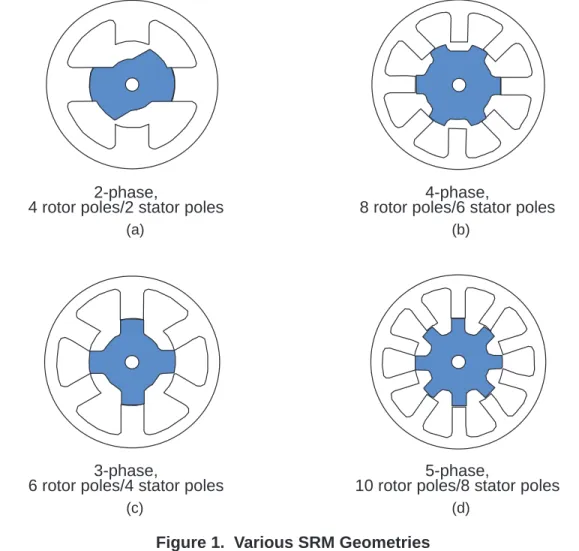
By varying the number of phases, the number of stator poles, and the number of rotor poles,
many different SRM geometries can be realized. A few examples are shown in Figure 1.
2-phase,
4 rotor poles/2 stator poles
(b)
(a)
4-phase,
8 rotor poles/6 stator poles
3-phase,
6 rotor poles/4 stator poles
(c)
(d)
5-phase,
10 rotor poles/8 stator poles
Figure 1. Various SRM Geometries
Note that although true of these examples, the number of phases is not necessarily equal to half
the number of rotor poles.
Generally, increasing the number of SRM phases reduces the torque ripple, but at the expense
of requiring more electronics with which to operate the SRM. At least two phases are required to
guarantee starting, and at least three phases are required to insure the starting direction. The
number of rotor poles and stator poles must also differ to insure starting.
2.1
Torque-Speed Characteristics
The torque-speed operating point of an SRM is essentially programmable, and determined
almost entirely by the control. This is one of the features that makes the SRM an attractive
solution. The envelope of operating possibilities, of course, is limited by physical constraints
such as the supply voltage and the allowable temperature rise of the motor under increasing
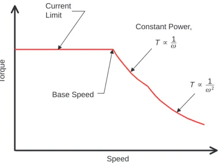
load. In general, this envelope is described by Figure 2.
T
orque
Speed
Base Speed
Current
Limit
Constant Power,
T
T
w
1
T
T
1
w
2Figure 2. SRM Torque-Speed Characteristics
Like other motors, torque is limited by maximum allowed current, and speed by the available bus
voltage. With increasing shaft speed, a current limit region persists until the rotor reaches a
speed where the back-EMF of the motor is such that, given the DC bus voltage limitation we can
get no more current in the winding—thus no more torque from the motor. At this point, called the
base speed, and beyond, the shaft output power remains constant, and at it’s maximum. At still
higher speeds, the back-EMF increases and the shaft output power begins to drop. This region
is characterized by the product of torque and the square of speed remaining constant.
2.2
Electromagnetic Equations
Although SR motor operation appears simple, an accurate analysis of the motor’s behavior
requires a formal, and relatively complex, mathematical approach. The instantaneous voltage
across the terminals of a single phase of an SR motor winding is related to the flux linked in the
winding by Faraday’s law,
v
+
iRm
)
d
f
dt
where, v
is the terminal voltage, i
is the phase current, R
m
is the motor resistance, and
φ
is the
flux linked by the winding. Because of the double salient construction of the SR motor (both the
rotor and the stator have salient poles) and because of magnetic saturation effects, in general,
the flux linked in an SRM phase varies as a function of rotor position,
θ
, and the motor current.
Thus, Equation (1) can be expanded as
v
+
iRm
)
ē
f
ē
i
di
dt
)
ē
f
ē
q
d
q
dt
where,
ē
ē
f
i
is defined as L(
θ
, i), the instantaneous inductance,
ē
ē
f
q
is K
b
(
θ
, i), the instantaneous
back EMF.
(1)
2.3
General Torque Equation
Equation (2) governs the transfer of electrical energy to the SRM’s magnetic field. In this section,
the equations which describe the conversion of the field’s energy into mechanical energy are
developed. Multiplying each side of Equation (1) by the electrical current, i, gives an expression
for the instantaneous power in an SRM,
vi
+
i
2Rm
)
i
d
f
dt
The left-hand side of Equation (3) represents the instantaneous electrical power delivered to the
SRM. The first term in the right-hand side (RHS) of Equation (3) represents the ohmic losses in
the SRM winding. If power is to be conserved, then the second term in the RHS of Equation (3)
must represent the sum of the mechanical power output of the SRM and any power stored in the
magnetic field. Thus,
i
d
f
dt
+
dW
mdt
)
dW
fdt
where,
dW
mdt
is the instantaneous mechanical power, and
dW
fdt
is the instantaneous power, which
is stored in the magnetic field. Because power, by it’s own definition, is the time rate of change
of energy, W
m
is the mechanical energy and W
f
is the magnetic field energy.
It is well known that mechanical power can be written as the product of torque and speed,
dWm
dt
+
T
w
+
T
d
q
dt
where, T is torque, and
w
+
d
q
dt
is the rotational velocity of the shaft.
Substitution of Equation (5) into Equation (4) gives,
i
d
f
dt
+
T
d
q
dt
)
dW
fdt
and solving Equation (6) for torque yields the equation,
T (
q
,
f
)
+
i (
q
,
f
)
d
f
d
q
*
dW
f(
q
,
f
)
d
q
and for constant flux, Equation (7) simplifies to,
T
+ *
ē
ē
W
q
fSince it is often desirable to express torque in terms of current rather than flux, it is common to
express torque in terms of co-energy, W
c
, instead of energy. To introduce the concept of
co-energy, first consider a graphical interpretation of field energy. For constant shaft angle,
d
q
dt
+
0
,
integration of Equation (6) shows that the magnetic field energy can be given by the
equation,
W
f+
ŕ
f 0i(
q
,
f
)
d
f
(3)
(4)
(5)
(6)
(7)
(8)
(9)
and graphically by the shaded area in Figure 3.
φ
Flux Linkage
i
Current
for angle,
θ
,
magnetization
curve defines
current as a
function of flux
i = i (
θ
,
φ
)
W
f, stored field energy
Figure 3. Graphical Interpretation of Magnetic Field Energy
Now, consider Figure 4.
φ
Flux Linkage
i
Current
for angle,
θ
,
magnetization
curve defines flux
as a function of
current
φ
=
φ
(
θ
,i )
W
c, stored field co-energy
For the fixed angle,
θ
, let the magnetization curve define flux as a function of current, instead of
current defined as a function of flux. The shaded area below the curve,
Wc
+
ŕ
i0
(
,
i) di
is defined as the magnetic field co-energy.
From Figure 3 and Figure 4, we see that the area defining the field energy and co-energy can be
described by the relation,
Wc
)
W
f+
i
Differentiating both sides of Equation (11) yields
dWc
)
dW
f+
di
)
id
Solving for the differential field energy in Equation (12) and substituting back into Equation (7)
gives,
T
+
id
* ǒ
di
)
id
*
dW
c(
,
i)
Ǔ
d
For simplification, the general torque equation, Equation (13), is usually simplified for values of
constant current. The differential co-energy can be written in terms of its partial derivatives as,
dWc
(
,
i)
+ ē
ē
Wc
d
) ē
Wc
ē
i
di
From Equation (13) and Equation (14), it is fairly easy to show that under constant current,
T
+ ē
Wc
ē
,
i constant
2.4
Simplified Torque Equation
Often, SRM analysis proceeds under the assumption that, magnetically, the motor remains
unsaturated during operation. This assumption can be useful for “first cut” control designs or
performance predictions. When magnetic saturation is neglected, the relationship from flux to
current is given by,
+
L(
)
@
i
and the motor inductance varies only as a function of rotor angle. Substituting Equation (16) into
Equation (10) and evaluating the integral yields,
W
c+
i
22
L(
)
and then substituting Equation (17) into Equation (15) gives the familiar simplified relationship
for SRM torque,
T
+
i
22
dL
d
(10)
(11)
(12)
(13)
(14)
(15)
(16)
(17)
(18)
3
Control
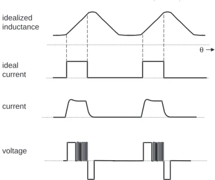
SRM drives are controlled by synchronizing the energization of the motor phases with the rotor
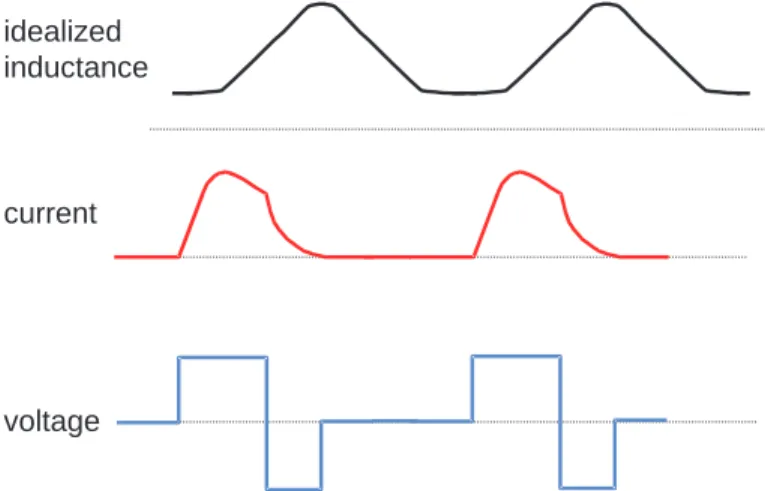
position. Figure 5 illustrates the basic strategy.
θ
idealized
inductance
ideal
current
current
voltage
Figure 5. Basic Operation of a Current-Controlled SRM – Motoring at Low Speed
As Equation (18) suggests, positive (or motoring) torque is produced when the motor inductance
is rising as the shaft angle is increasing,
dL
d
0
.
Thus, the desired operation is to have current in the SRM winding during this period of time.
Similarly, a negative (or braking) torque is produced by supplying the SRM winding with current
while
dL
d
0
.
The exact choice of the turn-on and turn-off angles and the magnitude of the phase current,
determine the ultimate performance of the SRM. The design of commutation angles, sometimes
called firing angles, usually involves the resolution of two conflicting concerns
−
maximizing the
torque output of the motor or maximizing the efficiency of the motor. In general, efficiency is
optimized by minimizing the dwell angle (the dwell angle is the angle traversed while the phase
conducts), and maximum torque is achieved by maximizing the dwell angle to take advantage of
all potential torque output from a given phase.
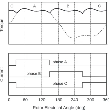
T
orque
Rotor Electrical Angle (deg)
Current
0
60
120
180
240
300
360
C A B C phase A phase C phase BFigure 6. Commutation of a 3-Phase SRM
In the top plot of Figure 6, the dashed line shows the torque that would be generated by phase
A, should constant current flow through the phase winding during an entire electrical cycle of the
SRM. With the idealized current waveforms of the figure, the resulting net torque from the motor
is shown by the solid line. The turn-on and turn-off angles coincide with the region where
maximum torque is obtained for the given amount of phase current.
This commutation sequence tends to optimize efficiency. Here, a dwell angle of 120 electrical
degrees is used, which is the minimum dwell angle that can be used for a three-phase SRM,
without regions of zero torque.
Of interest to note from Figure 6 is that constant current results in non-constant torque. As might
be expected, schemes have been proposed by Husain and Ehsani
1
, Ilic-Spong, et al
2
, and
Kjaer, et al
3
that attempt to linearize SRM output torque by shaping and controlling the phase
currents through some non-linear function that depends upon the motor characteristics. This
application, although not covered in this report, is well suited for DSP implementation.
Figure 6 illustrates the effect that the choice of commutation angles can have upon the SRM
performance. Equally important is the magnitude of the current that flows in the winding.
Commonly, the phase current is sensed and controlled in a closed-loop manner, and as seen in
the voltage curve of Figure 5, the control is typically implemented using PWM techniques.
1
I. Husain and M. Ehsani, ” Torque Ripple Minimization in Switched Reluctance Motor Drives by
PWM Current Control,” Proc. APEC’94, 1994, pp. 72–77.
2
M. Ilic-Spong, T. J. E. Miller, S. R. MacMinn, and J. S. Thorp, “Instantaneous Torque Control of
Electric Motor Drives,” IEEE Trans. Power Electronics, Vol. 2, pp. 55–61, Jan. 1987.
3
P. C. Kjaer, J. Gribble, and T. J. E. Miller, “High-grade Control of Switched Reluctance Machines,”
SRM control is often described in terms of ”low-speed” and ”high-speed” regimes. Low-speed
operation is typically characterized by the ability to arbitrarily control the current to any desired
value. Figure 5 illustrates waveforms typical of low-speed SRM operation. As the motor’s speed
increases, it becomes increasingly difficult to regulate the current because of a combination of
the back EMF effects and a reduced amount of time for the commutation interval. Eventually a
speed is reached where the phase conducts (remains on) during the entire commutation
interval. This mode of operation, depicted by Figure 7, is called the single-pulse mode.
idealized
inductance
current
voltage
Figure 7. Single-Pulse Mode – Motoring, High Speed
When this occurs, the motor speed can be increased by increasing the conduction period (a
greater dwell angle) or by advancing the firing angles, or by a combination of both. By adjusting
the turn-on and turn-off angles so that the phase commutation begins sooner, we gain the
advantage of producing current in the winding while the inductance is low, and also of having
additional time to reduce the current in the winding before the rotor reaches the negative torque
region. Control of the firing angles can be accomplished a number of ways, and is based on the
type of position feedback available and the optimization goal of the control, as discussed in
publications by Becerra, et al,
4
and Miller.
5
When position information is more precisely known,
a more sophisticated approach can be used. One approach is to continuously vary the turn-on
angle with a fixed dwell.
Near turn-on, Equation (2) can be approximated as
v
i
di
dt
Lu
di
dt
4
R. Becerra, M. Ehsani, and T. J. E. Miller, “Commutation of SR Motors,” IEEE Trans. Power
Electronics, Vol. 8, July 1993, pp. 257–262.
5
T. J. E. Miller, “Switched Reluctance Motors and Their Control,” Magna Physics Publishing,
Hillsboro, OH, and Oxford, 1993.
Multiplying each side of Equation (19) by the differential, d
θ
, and solving for d
θ,
gives,
d
Lu
v
di
d
dt
and using first order approximations yields an equation for calculating advance angle,
adv
Lu
i
cmdV
buswhere i
cmd
is the desired phase current and V
bus
is the DC bus voltage.
4
Example – SRM Drive with Position Feedback
This section describes an example application of an SRM drive with position feedback. The
SRM is a 3-phase 12/8 machine that is speed and current controlled.
4.1
Hardware Description
4.1.1
SRM Characteristics
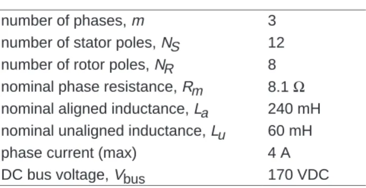
The characteristics of the SRM used in this application report are given by Table 1.
Table 1. SRM Parameters
number of phases, m
3
number of stator poles, N
S12
number of rotor poles, N
R8
nominal phase resistance, R
m8.1
Ω
nominal aligned inductance, L
a240 mH
nominal unaligned inductance, L
u60 mH
phase current (max)
4 A
DC bus voltage, V
bus170 VDC
4.1.2
Control Hardware
The control hardware used in this application report is the TMS320F240 evaluation module
(EVM).
4.1.3
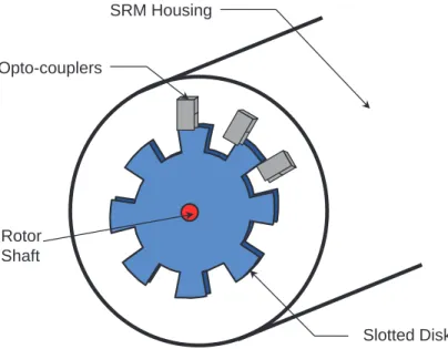
Position Sensor
Shaft position information is provided using an 8-slot, slotted disk connected to the rotor shaft
and three opto-couplers mounted to the stator housing as shown in Figure 8.
(20)
SRM Housing
Opto-couplers
Rotor
Shaft
Slotted Disk
Figure 8. SRM Shaft Position Sensor
The opto-couplers are nominally located 30
°
apart from each other along the circumference of
the disk. This configuration and geometry produces the output waveforms shown in Figure 9.
Opto #1 Opto #2 Opto #3 (mechanical angle) (electrical angle) 0 15 30 45 0 120 240 360/0
Figure 9. Opto-Coupler Output Signals vs. Rotor Angle
This configuration generates an opto-coupler edge for every 7.5
°
of mechanical rotation. For
every 45
°
of mechanical rotation the signal pattern repeats, corresponding to one electrical cycle
of the SRM, of which there are 8 per shaft revolution.
In this report both mechanical angle and electrical angle are referenced. Mechanical angle is
useful when considering velocity control of the SRM, and electrical angle is convenient when
considering commutation. Electrical angle is related to mechanical angle by the number of rotor
poles, N
R
. In Figure 9, the angles are arbitrarily defined with respect to some convenient point.
Here, 180
°
electrical is defined as the aligned position for phase A of the motor. This is easily
verified by energizing phase A and then monitoring the opto-coupler output waveforms on an
oscilloscope to observe that the rotor is at the point where opto-coupler #3 switches state, while
opto-coupler #2 is low and opto-coupler #1 is high. For a 3-phase SRM, phases B and C are
related to the position of phase A by adding 120 and 240 electrical degrees, respectively.
A fundamentally identical position sensor can be implemented by replacing the opto-couplers
with Hall-effect sensors and embedding permanent magnets within the teeth of the slotted disk.
The opto-couplers are connected to the F240 EVM as shown in Figure 10.
Opto-coupler #x
+5 V
CAPx
IOPx
x = 1,2,3
Figure 10. Opto-Coupler Connections to the TMS320F240 EVM
Here, each opto-coupler output is connected to both a capture input and a digital I/O input. As
will be explained in further detail below, the capture inputs are used once the motor is running,
and the digital I/O inputs are used for estimating initial rotor position and for starting the SRM.
4.1.4
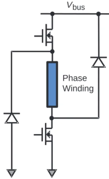
Power Electronics Hardware
The amount of current flowing through the SRM windings is regulated by switching on or off
power devices, such as MOSFETs or IGBTs, which connect each SRM phase to a DC bus. The
power inverter topology is an important issue in SRM control because it largely dictates how the
motor can be controlled.
There are numerous options available, and invariably the decision will come down to trading off
the cost of the driver components against having enough control capability (independent control
of phases, current feedback, etc.) built into the driver. A popular configuration, and the one used
in this application report, uses 2 switches and 2 diodes per phase. This topology is depicted in
Figure 11.
Phase
Winding
V
busFigure 11. Two-Switch Per Phase Inverter
Publications by Vukosavic and Stfanovic
6
and Miller
7
offer several other configurations that
require fewer switches per phase, although with some penalty on control flexibility and
maintaining phase independence. A gate drive IC device, such as the IR2110, is used to turn on
and off the semiconductor switches. In the topology of Figure 11, the low-side switch is usually
held on during a commutation interval, while the top switch is used to implement the control. For
independent current control of each phase, a low-ohm sense resistor is placed between the
source of the low-side n-channel power MOSFET and ground.
A schematic diagram of the inverter used in this application report, including the gate drive
circuit and the connections to the EVM, is given in Figure 12.
6
S. Vukosavic and V. Stfanovic, “SRM Inverter Topologies: A Comparative Evaluation,” IEEE IAS
Annual Meeting Conf. Record, 1990.
7
T. J. E. Miller (ed.), “Switched Reluctance Motor Drives,” Intertec Communications Inc., Ventura
_ + CMPj / PWM j CMPi / PWM i j = 2,4,6 i = 1,3,5 7403 1 2 4 5 3 6 3 5 MC14049 +15 IR2110 2 4 9 12 10 11 13 7 5 6 3 1 2 VDDHO LIN HIN SD VSS VB VS VCC LO COM 2.2 µF +15 22 +LOAD +VBUS –LOAD IRF740 IRF710 +15 IRFD123 10k HFA15TB60 HFA15TB60 22 IRF740 LOGIC GROUND SENSE RESISTOR ADCINx x = 1,2,3 POWER GROUND MUR160 0.01 µF
Figure 12. Schematic Diagram of SRM Inverter Using the IR2110 and Connections to the EVM
The diagram shows the components used for a single phase. Each phase uses two IRF740
n-channel power MOSFETs for the switching elements in the output stage. The IRF740 is rated
at 400 VDC, 10 A. The drain to source on resistance of these devices is 0.55
Ω
. The
free-wheeling diodes used in the power stage are HFA15TB60s, fast recovery diodes. The
HFA15TB60 has a reverse recovery time of 60 ns, and is rated at 600 VDC, 15 A. Logic is
implemented at the input to the gate drive IC such that the top power MOSFET can be turned on
only when the bottom MOSFET is also on. The reasons for this limitation, and other circuit
details, are discussed more thoroughly in a publication by Clemente and Dubhashi.
8
4.2
Software Description
The software described in this application report is written in C and is designed for operating a
3-phase 12/8 SRM in closed loop current control and closed loop speed control. A block diagram
of the algorithms implemented is given in Figure 13.
8
S. Clemente and A. Dubhashi, “HV Floating MOS-Gate Driver IC,” International Rectifier
}
on speed cmd + –P
I
torque cmd DSP icmd + –K
PWM Inverter SRM current controller velocity controller torque to current currentT
samp off commutation angles advance angle calc position estimator position edges opto-couplers position DC bus voltage velocity estimatorFigure 13. Block Diagram of the SRM Controller
Velocity is estimated by monitoring the elapsed time between opto-coupler edges, which are a
known distance apart. A velocity compensation algorithm determines the torque required to
bring the motor velocity to the commanded value.
A commutation algorithm converts the torque command into a set of phase current commands,
and the current in each phase is individually regulated using a fixed-frequency PWM scheme.
Further details on each of the algorithms are provided in subsequent sections of this report.
4.2.1
Program Structure
Figure 14 shows the structure of the SRM control software for the TMS320F240 DSP.
Start
Initialization Routines: – DSP Setup
– Event Manager Initialization – SRM Algorithm Initialization – Enable Interrupts – Start Background Run Routines: Background: – Velocity Estimation – Visual Feedback Timer ISR: – Current Control – Position Estimation – Commutation – Velocity Control Capture ISR: – Store Capture Data
– Schedule Position msmt Update – Schedule Velocity msmt Update
At the highest level, the software consists of initialization routines and run routines. Upon
completion of the necessary initialization, the background task is started. The background is
simply an infinite loop, although when required, lower priority processing including velocity
estimation and a visual feedback routine is executed. The velocity estimation involves
double-precision division arithmetic, thus it is executed in background mode so that the timeline
is not violated. This algorithm is initiated in the capture interrupt service routine. The visual
feedback function simply toggles an LED on the EVM board to provide a signal to the user that
the code is running.
All of the time critical motor control processing is done via interrupt service routines. The timer
ISR is executed at each occurrence of the maskable CPU interrupt INT3. This interrupt
corresponds to the event manager group B interrupts, of which we enable only the timer #3
period interrupt, TPINT3. The frequency, F, at which this routine is executed is specified by
loading the timer 3 period register with the desired value. The SRM control algorithms which are
implemented during the timer ISR are the current control, shaft position estimation,
commutation, and velocity control. As illustrated in Figure 15, only the current control and shaft
position estimation are executed at the frequency, F.
Î Î 5 1 2 3 4 5 1 2 3 4 ÏÏ ÏÏ ÏÏ ÏÏ ÌÌ ÌÌ Ì Ì Î Î ÎÎ ÎÎ ÑÑ ÑÑ ÑÑ ÑÑ ÓÓ ÓÓ ÔÔ ÔÔ ÖÖ ÖÖ ÏÏ ÏÏ ÒÒ ÒÒ Ó Ó ÕÕ ÕÕ ÕÕ ÕÕ ÎÎ ÎÎ Î Î Ó Ó ÓÓ ÓÓ ŠŠ ŠŠ ŠŠ ŠŠ ÚÚ ÚÚ ÛÛ ÛÛ ÜÜ ÜÜ Timer ISR Processing Capture ISR Processing Background Processing Total Processing capture interrupts
timer 3 period interrupts
current control and position estimation commutation
velocity control
read and store capture data velocity estimation
Figure 15. Processor Timeline Showing Typical Loading and Execution of
SRM Control Algorithms
Because of their lower bandwidth requirements, velocity control and commutation are performed
at a frequency of F/5. Considering the timer ISR as being sliced into fifths with a pattern
repeating every five slices, commutation is run only in the first slice and the velocity loop only in
the second. Current control and position estimation are performed in each slice.
The capture interrupt service routine is executed at each occurrence of the maskable CPU
interrupt INT4. This CPU interrupt corresponds to the event manager group C interrupts, of
which we enable the three capture event interrupts, CAPINT1–3. This ISR executes
asynchronously to the timers on board the DSP and the frequency of execution is dependent on
the SRM shaft speed according to the equation,
capture ISR frequency (Hz)
shaft speed (rpm)
360 (deg)
(rev)
1
7.5 (deg)
1 (min)
60 (sec)
The capture ISR is used to determine which capture interrupt has occurred, read the appropriate
capture FIFO register, and then store the data. Although no algorithm is explicitly executed in
this ISR, flags are set which initiate velocity and position estimation actions. As described above,
the velocity estimate update calculation is performed in the background. The position estimation
algorithm, which executes during the timer ISR, is notified that a new position measurement has
been received.
Table 2 summarizes the processing requirements for each of the major software functions for the
SRM controller.
Table 2. Benchmark Data for the Various SRM Drive Software Modules
S/W Block
Module
Number of
Cycles
Execution
Time
@ 50 ns
Execution
Frequency
Relative
Time
@ 5 kHz
Velocity Estimation
Background
3620
181.0
µ
s
800 Hz
†29.0
µ
s
Visual Feedback
Background
60
3.0
µ
s
2 Hz
0.0
µ
s
Current Control
Timer ISR
948
47.4
µ
s
5000 Hz
47.4
µ
s
Position Estimation
Timer ISR
258
12.9
µ
s
5000 Hz
12.9
µ
s
Commutation
Timer ISR
1296
64.8
µ
s
1000 Hz
13.0
µ
s
Velocity Control
Timer ISR
444
22.2
µ
s
1000 Hz
4.4
µ
s
Misc. Overhead
Timer ISR
140
7.0
µ
s
5000 Hz
7.0
µ
s
Capture ISR
Capture ISR
500
25.0
µ
s
800 Hz
†4.0
µ
s
C Context Switch
RTS.LIB
120
6.0
µ
s
5800 Hz
7.0
µ
s
Total
124.7
µ
s
† at a shaft speed of 1000 rpm
The data in Table 2 shows that when the timer ISR frequency, F, is chosen as 5 kHz, that the
overall processor loading is equal to
processor loading
124.7 s
200.0 s
62.4% ,
when running the DSP at a 20 MHz clock frequency. The code size is 2456 words and
167 words are required for variable/data storage. Thus, the total memory requirement is less
than 3K words. Complete code listings are given in Appendix A.
It should be noted that this benchmark data was taken with the program and data memory
located off chip, as can be seen in the link.cmd file located in the appendix. A 2
×
to 3
×
improvement in execution can be achieved by moving the .bss and .stack sections of the
firmware to the on-chip B0/B1 area of the DSP and by moving the .text section of the firmware to
the flash memory.
(22)
4.2.2
Initialization Routines
A flowchart describing the initialization routines is given in Figure 16.
disable interrupts
reset
DSP setup
disable interrupts
initialize event
manager
initialize
SRM algroithm
parameters
initialize program
control counters
and flags
enable interrupts
start background
Figure 16. Initialization Flowchart
The DSP is configured so that the watchdog timer is disabled. The TMS320F240 EVM has a
10 MHz crystal, which is used in conjunction with the PLL module of the DSP to yield a 20 MHz
CPUCLK.
The event manager initialization configures the timer units, the capture units, the compare units,
and the A/D converters. Also, the CAP1–CAP4 and IOPB0–IOPB3 pins, whose functions are
software programmable, are configured to operate as capture pins and digital output pins,
respectively.
Each of the timers are programmed to operate in the continuous up count mode. Timer #1
provides the timebase for the fixed-frequency PWM control of the phase current. Timer #2
provides the timebase for the capture events, and timer #3 is used to provide a CPU interrupt at
a fixed rate. The compare units are configured to the PWM mode, where PWMs 1,3, and 5
(used for switching the high-side power MOSFET) are configured as active high.
The SRM algorithm initialization defines the parameters of the position estimation state machine
and sets the initial conditions of the motor, for example, setting the shaft velocity estimate to
zero. Also, during this routine, the logic states of the opto-couplers are read from the digital I/O
pins, and this information used to estimate the rotor position.
Upon initializing several flags and counters which are used for program flow control, the infinite
loop background routine is called, and the normal operation of controlling the SRM drive begins.
See the comments in the code listings found in Appendix A for further information on the
program initialization.
4.2.3
Current Controller
Current is regulated by fixed-frequency PWM signals with varying duty cycles. The
TMS320F240 accomplishes this using compare units and output logic circuits. The compare
units are programmed for PWM mode, to use timer #1 as a time base. The desired output logic
polarity is controlled by the ACTR register. The PWM frequency is specified by loading the
period register of timer #1, T1PER, with a value, P, defined by,
P
+
CPUCLK frequency
PWM frequency
*
1
For the F240, the CPUCLK frequency is 20 MHz. The percentage duty cycle for the x
th
phase is
controlled by loading the appropriate compare register, CMPRx, with an appropriate value
between 0 and P (0 = 0%, P/2 = 50%, P = 100%). A PWM frequency of 20 kHz is used. The
value is significantly higher than the bandwidth of the current loop and also at a frequency which
is inaudible.
The percentage duty cycle command is calculated by the current loop compensation algorithm,
which is designed using linear analysis. The analysis begins with an approximate model of the
current loop, given by Figure 17.
Current Control Algorithm Loop Gain
i
cmd K P 01
P
PWMV
bus SRM V1
ń
R
m i(L
ń
R
m)s
)
1
i
fb1
*
e
*sTs
ZOH A/D Converter
Feedback Gain 1023 0
1023
5
K
fbFigure 17. Approximate SRM Current Loop Model
Using the SRM data of Table 2, and with P = 999, K
fb
= 1.17 V/A, the open-loop frequency
response, G(
ω
), of the SRM current loop, from i
cmd
to i
fb
, is given in Figure 18 for values of
phase inductance at both the aligned rotor position (L = L
a
) and the unaligned rotor position
(L = L
u
).
0
Phase (deg) DC gain = 14.1 dB + 20log10(K) Magnitude (dB) –100 –200 10 100 1000 104 Frequency (Hz) desired 0 dB 1.16 decade slope = –20 dB/decade 370 Hz R Lmin +200 radńs (32 Hz) desired P.M. = 65 deg –180 degFigure 18. Frequency Response Plots for the SRM Current Loop at the Unaligned Position
(Squares) and at the Aligned Position (Circles)
Because of the digital implementation of the current loop, additional phase loss, beyond the 90
°
due to the motor pole, is contributed by the sample and hold process and the processing delay
inherent in the loop. These dynamics essentially limit the current loop bandwidth to an open loop
crossover frequency near 370 Hz. The time delay due to the zero-order hold (ZOH) is equal to
½
of the sampling period, in this case
½
of 200
µ
sec, or 100
µ
sec. Since the phase loss at any
frequency,
ω
, due to a pure time delay,
τ
, is given by the expression,
q
loss+
wt
using Equation (25), we calculate that the phase loss due to the ZOH sampling at 370 Hz is
equal to
q
loss+
2
p
370
ǒ
100
10
*6Ǔ
+
0.232 rad
+
13.3
oAssuming that the processing delay is equal to 50% of a loop cycle, or another 100
µ
sec, then
the net effect of digital implementation yields about 26
°
of phase loss at 370 Hz. When
combined with the 90
°
due to the motor pole, the phase loss through the loop is approximately
116
°
, at 370 Hz. If the loop gain, K, is chosen such that the 0 dB point of the open-loop
magnitude occurs at 370 Hz, then the resulting phase margin in the loop will be about 64
°
. This
amount of phase margin provides a very stable loop design. The DC gain of the loop is given by,
(25)
K
@
V
bus@
K
fb@
1023
P
@
5
@
R
+
5.092
K
which, when written in decibels, is equal to,
DC gain
+
14.1 dB
)
20 log
10(K)
For frequencies where
ω >
(R/L), the magnitude of the loop response is equal to,
|G( )|
+
14.1 dB
)
20 log
10(K)
*
2
ǒ
R
ń
L
Ǔ
In Equation (29), letting L = L
u
provides the most conservative choice, resulting in a stable
design for all rotor positions. Setting the left-hand side of Equation (29) to 0 dB while
ω
=
2
π
(370) rad/s, and solving for K, yields the value of K which ensures the desired open-loop
crossover point for the current loop. In this case K = 2.8.
Often, a PI controller is used. In this example adding an integrator to the control law will not
make much difference in the loop performance, except only at very low speeds, because the
integrator action must be slower than the motor pole to stabilize the loop. In this example using a
3-phase, 12/8 SRM, the motor pole is located near 32 Hz. The SRM operating speed required to
produce the equivalent of 32 Hz commands to the SRM current loops is 240 rpm. Thus, in this
case, only at operating speeds lower than 240 rpm would any integrator action be helpful.
The current loop gain is set using the ILOOP_GAIN constant in the file CONSTANT.H. For this
value, Q3 scaling is used, thus setting ILOOP_GAIN = 22 results in K = 2.75, which is
sufficiently close to the desired value of 2.8, for this application.
4.2.4
Position Estimation
Recall that Figure 9 showed six possible combinations of the opto-coupler output states per
electrical cycle of the SRM. The transitions of the outputs define specific angles. This
information can readily be described by a state machine, such as Figure 19.
011 [3] 0° 001 [1] 101 [5] 100 [4] 110 [6] 010 [2] 60° 300° 120° 180° 240° Opto #1 Opto #3 Opto #2 Opto #2 Opto #3 Opto #1
Figure 19. State Transition Diagram for the SRM Position Pickoff
(27)
(28)
The state, [ ], is defined by ‘zyx’, where z is the logic state of opto-coupler #3, y of
opto-coupler #2, and x is the state of opto-coupler #1.
Position measurements are made by using this state machine and identifying which opto-coupler
transition occurs, using the DSP’s capture units.
The opto-couplers and slotted disk provide position measurements at six discrete points per
electrical cycle of the SRM. Many commutation schemes, however, require continuous position
information to optimize performance. Thus, to provide a position estimate between
measurements, the equation,
q
^(k)
+
q
^(k
*
1)
)
w
^f(k)
1
fs
is used, where f
s
is the estimation update rate and
k
represents the time of the most recent
capture edge. Equation (30) is implemented, using double precision arithmetic, as follows:
long dp; /* delta–position in mechanical angle */ int speed;
int temp;
if (anSRM–>wEst_10xrpm > 0) {
dp = anSRM–>wEst_10xrpm * K_POSITION_EST + anSRM–>dp_remainder; anSRM–>dp_remainder = dp & 0xffff;
temp = (int) (dp >> 16);
anSRM–>position = anSRM–>position + (temp * NR); }
else {
speed = –anSRM–>wEst_10xrpm;
dp = speed * K_POSITION_EST + anSRM–>dp_remainder; anSRM–>dp_remainder = dp & 0xffff;
temp = (int) (dp >> 16);
anSRM–>position = anSRM–>position – (temp * NR);
}
The constant K_POSITION_EST (Q16), compensates for units (shaft velocity is available in the
software as
SRM.wEst_10xrpmwith units of rpm
×
10) and is calculated according to the equation,
K_POSITION_EST
+
1
10
(rpm
10)
1 (sec)
fs
1 (min)
60 (sec)
360
o(rev)
65535
360
o2
16for, f
s
= 5 kHz, K_POSITION_EST = 1432.
During startup, the digital I/O ports determine the state of the rotor and initial position is
estimated in the mid-range of the state. For example, a reading of [100], (consistent with
Figure 19) yields an initial position estimate of 270 electrical degrees. The capture units provide
subsequent measurements, by recognizing the edges, or state transitions.
4.2.5
Velocity Estimation
The three opto-coupler outputs produce an edge every 7.5
°
of mechanical rotation, and each
opto-coupler produces an edge every 22.5
°
mechanical. At each edge, velocity is calculated
according to the equation,
w
^+
Dq
D
t
+
60
@
Dq
@
f
clkN
(30)
(31)
(32)
where,
w
^is the velocity estimate (rpm)
Dq
is the distance between opto-coupler edges (rev)
D
t
is the time between edges (min)
N is the number of clock counts between edges
f
clk
is the clock frequency (Hz)
The time between edges is determined from the capture units. The capture units are
programmed via the CAPCON register to use timer #2 as a time base, and to trigger on both
rising and falling edges. Timer #2 is programmed to count at 1.25 MHz via the T2CON. Although
we trade-off resolution in measuring
∆
t, a clock frequency of 1.25 MHz is chosen, versus a
maximum of 20 MHz, so that the 16-bit registers containing the count do not overflow except at
very low speeds. Using a 1.25 MHz clock, the counter overflows only at shaft speeds less than
71.5 rpm, considered very low for our application. So that we can operate (although degraded)
at speeds lower than about 100 rpm,
∆
t
in Equation (32) is determined by a software counter of
the number of 5 kHz timer interrupts that occur between opto-coupler edges.
It can be shown that when instantaneous velocity is estimated by Equation (32) that the
quantization of a velocity estimate is given by
Q
+
d
w
^dN
+
w
2
60
@
Dq
@
f
clkand, Q is the quantization of velocity (rpm). In our design,
∆θ
= 1/16 revolution (22.5
°
mechanical) and f
clk
= 1.25 MHz. Thus, at 1200 rpm, the quantization is 0.31 rpm.
Various filtering can be applied to Equation (32) for smoothing the velocity estimate, depending
upon the application. What has proven useful is a combination of FIR and IIR filtering of the
form:
w
^ f(k)
+
a
@
w
^ f(k
*
1)
)
(1
*
a
)
@
ȍ
k j+(k*5)w
^(
j)
The FIR filter portion of Equation (34) uses six (from
k
*
5
to
k
) instantaneous velocity
estimates. Because there are six opto-coupler edges per electrical cycle, once per cycle
estimation errors are removed.
(33)
The FIR filtering and the determination of the instantaneous velocity estimate is calculated using
double precision as follows:
DWORD a1,a2,a3,a4,a5,a6; DWORD sum_cnt;
int inst_velocity;
/*–––––––––––––––––––––––––––––––––––––––––––*/ /* Obtain instantaneous velocity estimate */ /*–––––––––––––––––––––––––––––––––––––––––––*/ if (mode == 1) {/* use timer #2 as time base */
/*–––––––––––––––––––––––––––––––––––––––––––––––––––*/ /* FIR filter for removing once per electrical cycle */ /* effects */ /*–––––––––––––––––––––––––––––––––––––––––––––––––––*/ a1 = (DWORD) anSRM–>capture_delta[0][0]; a2 = (DWORD) anSRM–>capture_delta[0][1]; a3 = (DWORD) anSRM–>capture_delta[1][0]; a4 = (DWORD) anSRM–>capture_delta[1][1]; a5 = (DWORD) anSRM–>capture_delta[2][0]; a6 = (DWORD) anSRM–>capture_delta[2][1]; sum_cnt = a1+a2+a3+a4+a5+a6; /*––––––––––––––––––––––––––––––––––––––––––––––––––––––*/ /* apply “velocity = delta_theta/delta_time” algorithm */ /*––––––––––––––––––––––––––––––––––––––––––––––––––––––*/ sum_cnt = K1_VELOCITY_EST/sum_cnt;
inst_velocity = ((int) sum_cnt) * anSRM–>shaft_direction; }
else { /* else, use timer ISR count as time base */ /*––––––––––––––––––––––––––––––––––––––––––––––––––––––*/ /* apply “velocity = delta_theta/delta_time” algorithm */ /*––––––––––––––––––––––––––––––––––––––––––––––––––––––*/ sum_cnt = K2_VELOCITY_EST/anSRM–>delta_count;
inst_velocity = ((int) sum_cnt) * anSRM–>shaft_direction; }
Here, K1_VELOCITY_EST and K2_VELOCITY_EST are constants which incorporate
∆θ
and
units so that the instantaneous velocity estimate has units of (rpm
×
10). The constants are
calculated using,
K1_VELOCITY_EST
6
22.5 (deg)
1.25e6 (cnts)
(sec)
1 (rev)
360 (deg)
60 (sec)
(min)
10
K2_VELOCITY_EST
1
7.5 (deg)
5000 (cnts)
(sec)
1 (rev)
360 (deg)
60 (sec)
(min)
10
(35)
The IIR filtering is implemented as:
long filt_velocity;/*–––––––––––––––––––––––––––––––––––––––––––––––––––*/ /* IIR filter for smoothing velocity estimate */ /*–––––––––––––––––––––––––––––––––––––––––––––––––––*/ filt_velocity = (ALPHA * anSRM–>wEst_10xrpm)
+ (ONE_MINUS_ALPHA * inst_velocity);
anSRM–>wEst_10xrpm = (int) (filt_velocity >> 3);
The filter coefficient,
α
, is chosen equal to 0.875, [ALPHA = 7 (Q3)]. Let
α
approach zero for a
higher bandwidth velocity estimate (less smoothing, more noise) and let
α
approach one for
more smoothing, less noise, and lower bandwidth.
4.2.6
Commutation
The commutation strategy ultimately determines the performance of the SRM. Torque-speed
range, machine efficiency, torque ripple, and acoustic noise all depend, to some extent, on the
commutation algorithm. Design of the commutation algorithm must consider requirements in
each of these areas, while trading off cost issues such as the algorithm complexity and the
availability or accuracy of various sensors. For a current controlled SRM, commutation can be
described as the transformation of the desired net motor torque into a set of desired phase
currents. This is described mathematically by the equation,
i
jcmd
+
g
j(
@
)
T
cmdand j = 1,...,m and m is the total number of motor phases. In general, g( ), is a non-linear
function of shaft angle
θ
, shaft speed
ω
, the desired torque command T
cmd
, the DC bus voltage
V
bus
, and the motor instantaneous inductance, L. The most simple choice for g( ) is given by
g(
q
)
+
ȥȡȢ
1,
0,
q
ONv
q
t
(
q
ON)
dq
)
otherwise
where the dwell angle,
δθ
, must be at least equal to 360
°
/m (electrical), to avoid regions of zero
torque production. An example of commutation described by Equation (37) is illustrated by
Figure 6. The turn-on angle,
θ
ON
, is typically a few degrees beyond the unaligned position of a
phase. Equation (37) is useful for only single-quadrant operation. For four quadrant operation,
Equation (37) must be modified, for example,
g(
q
,
T
cmd)
+
ȧ
ȧȥ
ȡ
Ȣ
1,
1,
0,
ƪ
q
ONv
q
t
(
q
ON)
dq
)
ƫ
&T
cmdu
0
otherwise
ƪ
(
q
ON)
p
)
v
q
t
(
q
ON)
p
)
dq
)
ƫ
&T
cmdt
0
(36)
(37)
(38)
where the conduction angles are offset by 180
°
electrical (
π
radians) when negative torque is
desired. This allows a phase to conduct during the region where
dL
d
q
< 0. An even more flexible
approach, which results in a wider operating range for the SRM, allows the turn-on and dwell
angles to vary. For example, Equation (38) is extended to allow
θ
ON
and
δθ
, to be functions of
velocity, desired torque, and the DC bus voltage.
Often, for minimizing torque ripple, the commutation is designed such that two phases conduct
simultaneously and share the job of producing the desired SRM torque. In this case,
Equation (38) is further extended to a function of the form,
g(
q
,
T
cmd)
+
ȧ
ȧ
ȥ
ȡ
Ȣ
ò
(
q
),
ò
(
q
),
0,
ƪ
q
ONv
q
t
(
q
ON)
dq
)
ƫ
&T
cmdu
0
ȧ
ȱ
Ȳ
(
q
ON)
p
)
v
q
q
t
(
q
ON)
p
)
dq
)
ȧ
ȳ
ȴ
&T
cmdt
0
otherwise
where
ρ
(
θ
) is the sharing function. Sharing functions are not implemented in this application
report, however, further information on the choice of sharing functions can be found in a
publication by Kjaer, et al.
9
Essentially commutation schemes of the form in Equation (39) use
knowledge of the motor characteristics to design a non-linear function,
ρ
(
θ
), that produces a
linear output torque.
In this example, the commutation coefficients, g( ), were calculated using Equation (38), where
θ
ON
=
π
/6 +
θ
adv
(radians),
δθ = π
/3 (radians), and the advance angle,
θ
adv
, is given by
Equation (21). This yields a single-quadrant, fixed-dwell, variable turn-on commutation
algorithm. This algorithm is implemented as follows:
int phase; WORD electricalAngle; WORD angle; int channel; long advance; /*–––––––––––––––––––––––––––*/ /* Advance angle calculation */ /*–––––––––––––––––––––––––––*/
advance = (anSRM–>wEst_10xrpm * anSRM–>desiredTorque); advance = advance >> 9;
/*–––––––––––––––––––––––––––––––––––––––––––––––––––––––*/ /* Offset for advance angle negative torque, if required */ /*–––––––––––––––––––––––––––––––––––––––––––––––––––––––*/ if (anSRM–>desiredTorque > 0) {
electricalAngle = anSRM–>position + (int) advance; }
else {
electricalAngle = anSRM–>position + PI_16 – (int) advance; }
9
P. C. Kjaer, J. Gribble, and T. J. E. Miller, pp. 1585–1593.
for (phase=0; phase< NUMBER_OF_PHASES; phase++) { /*––––––––––––––––––––––––––––––*/
/* 120 degree offsets for phase */ /*––––––––––––––––––––––––––––––*/
angle = electricalAngle – phase * TWOPIBYTHREE_16;
/*–––––––––––––––––––––––––––––––––––––––––––––––––––––––––––*/ /* turn phase on, if between desired angles and switch */ /* the mux on the A/D to measure the desired */
/* phase current */
/*–––––––––––––––––––––––––––––––––––––––––––––––––––––––––––*/ if ( (angle >= (PIBYSIX_16)) && (angle < (FIVEPIBYSIX_16)) ) { anSRM–>active[phase] = 1; channel = anSRM–>a2d_chan[phase]; switch_mux(channel,channel+8); } else { anSRM–>active[phase] = 0; } } }
As seen in the code above, the advance angle calculation (which yields an advance angle in
units of bits, 65535 bits = 360 electrical degrees) is computed according to the equation,
adv
(bits)
i
cmd(bits)
^(rpm
10)
K
,
K
2
9