Machine Learning manuscript No. (will be inserted by the editor) Multiclass Classification with Bandit Feedback using Adaptive

(1)

(will be inserted by the editor)

Multiclass Classification with Bandit Feedback using

Adaptive Regularization

Koby Crammer · Claudio Gentile

Received: date / Accepted: date

Abstract We present a new multiclass algorithm in the bandit framework, where after making a prediction, the learning algorithm receives only partial feedback, i.e., a single bit indicating whether the predicted label is correct or not, rather than the true label. Our algorithm is based on the second-order Perceptron, and uses upper-confidence bounds to trade-off exploration and exploitation, instead of random sampling as performed by most current al-gorithms. We analyze this algorithm in a partial adversarial setting, where instances are chosen adversarially, while the labels are chosen according to a linear probabilistic model which is also chosen adversarially. We show a regret of O(√TlogT), which improves over the current best bounds of O(T2/3_{) in} the fully adversarial setting. We evaluate our algorithm on nine real-world text classification problems and on four vowel recognition tasks, often obtain-ing state-of-the-art results, even compared with non-bandit online algorithms, especially when label noise is introduced.

Keywords First keyword·Second keyword·More

PACS PACS code1·PACS code2·more

Mathematics Subject Classification (2000) MSC code1·MSC code2 · more

1 Introduction

Consider a book recommendation system. Given a customer’s profile, it rec-ommends a few possible books to the user, with the aim of choosing books that

Koby Crammer

The Technion, Department of Electrical Engineering, Haifa, 32000, Israel E-mail: [email protected]

Claudio Gentile

Universita’ dell’Insubria, DICOM, Via Mazzini 5, 21100 - Varese, Italy E-mail: [email protected]

(2)

the user will like and eventually purchase. Typical feedback in such a system is the actual action of the user, or specifically what books has she bought, if any. The system cannot observe what would have been the user’s actions had other books got recommended.

Generally, such problems are referred to as learning with partial feedback. Unlike the full information case, where the system or the learning algorithm knows the outcome of each possible response, e.g., the user’s action for each and every possible book recommended, in the partial setting, the system observes the response only to very limited options and, in particular, the option that was actually recommended.

We consider an instantiation of this problem in the multiclass prediction problem within the online bandit setting. Learning is performed in rounds. On each round the algorithm receives an instance and outputs a label from a finite set of size K. It then receives a single bit indicating whether the predicted label is correct or not, which the algorithm uses to update its internal model and proceed to the next round. Note that for rounds where the feedback indicates wrong prediction, the algorithm’s uncertainty about the true label for that instance is almost not reduced, since the number of alternatives is only reduced fromK toK−1. Hence the algorithm needs somehow to follow an exploration-exploitation strategy.

Related work. Our algorithm trades-off exploration and exploitation via upper-confidence bounds, in a way that is somewhat similar to the work of Auer (2003) and Dani et al (2008). Yet, the result most closely related to our work is the Banditron algorithm of Kakade et al (2008), which builds on the immortal Perceptron algorithm. Kakade et al (2008) investigated this problem in an online adversarial setting, and showed a O(T2/3_{) bound on the regret} compared to the hinge loss of a linear-threshold comparator. Wang et al (2010) extended their results to a more general potential-based framework for online learning.

Multiclass classification with bandit feedback can be seen as a multi-armed bandit problem with side information. Relevant work within this research thread includes the Greedy-Epoch algorithm analyzed by Langford and Zhang (2007), where a O(T2/3_{) regret bound has been proven under i.i.d.} assump-tions, yet covering more general learning tasks than ours. We are aware of at least three more papers that define multi-armed bandit problems with side information, also called bandits with covariates: Wang et al (2005); Lu et al (2010); Rigollet and Zeevi (2010). However, the models in these paper are very different from ours, and not easily adapted to our multiclass problem. Another paper somewhat related to this work is by Walsh et al (2009), where the au-thors adopt a similar linear model as ours (and similar mathematical tools) in a setting where an online prediction algorithm is allowed to sometimes answer “I don’t know” (the so-called KWIK setting). A direct adaptation of their results to our multiclass setting is not straightforward. It is, however, easy to adapt their work to the binary (non-bandit) setting. In this case, their algo-rithm is shown to approximate the Bayes predictor with a convergence rate of

(3)

the formT−1/4. This result is significantly inferior to our convergence results, and it seems to hold only in the finite-dimensional case. We do not expect any multiclass adaptation of their results to lead to improved convergence rates.

Two papers (Valizadegan et al, 2011; Hazan and Kale, 2011) more closely related to our work became available after our paper was submitted; we briefly discuss these contributions in Section 8.

Our results. We study a setting related to the one by Kakade et al (2008) and Wang et al (2010), in which we assume a probabilistic linear model over the labels, although the instances are chosen by an adaptive adversary. We develop a bandit algorithm building on the 2nd-order Perceptron algorithm using the correlation matrix maintained by the algorithm to estimate uncer-tainty in prediction. We show regret bounds ofO(√TlogT), which are essen-tially optimal in this setting (up to log factors). We evaluate our algorithms on nine real-world text classification tasks and four vowel recognition tasks which vary in size, feature complexity and number of labels. We show that our algorithm always outperforms the Banditron algorithm. In fact, on a few datasets our algorithm also outperforms Perceptron and 2nd-order Perceptron working with full information labels, especially when label noise is induced. Finally, we sketch an extension of our results to the case when the labels have

anarbitrarydistribution, and an approximation error to our linear noise model

has to be taken into account.

2 Multiclass Bandit Online Learning

Standard online learning with full information is performed in rounds. On roundtthe algorithm receives an instancext∈Rdto be classified, and predicts

a label ˆy∈ {1. . . K}. It receives the true labelyt, updates its internal model,

and is ready for the next round.

The algorithm we present employs linear models. The algorithm maintains

Kweight vectorswi∈Rd, fori= 1, ..., K. Given an instancext, the algorithm

computes a score associated with each of theKclasses, defined byw>_i xt, and

outputs apredictionto be the label with the highest score, that is,

˜

yt= arg max i=1...Kw

>

i xt . (1)

We emphasize that two quantities are considered: the label with maximal score ˜

ytdefined in Eq. (1) (this quantity is internal to the algorithm), and the label

that is actually output by the algorithm, denoted by ˆyt. In the full-information

case, most algorithms just output their prediction, that is we have ˆyt = ˜yt.

In this paper, we focus on the partial information setting, also known as the

banditsetting. Here, after the algorithm makes a prediction, it does not receive

the correct label ytbut only a single bitMtindicating whether its output ˆyt

was correct or not, i.e.,

(4)

where{A}is 1 if the predicateAis true, and 0 otherwise.

Since learning algorithms receive only very limited feedback there is a nat-ural tradeoff between exploration and exploitation. On the one hand, the al-gorithm should output the best scoring label ˜yt = arg maxi=1...Kw>i xt, this

step being called exploitation. Yet, it may be the case that the model used at some point will not perform well (for example, the initial model), and thus the algorithm will make many mistakes and most of its feedback will indicate that the output is not correct, that is Mt= 1. This feedback is almost useless, as

there is still uncertainty about the true label (one ofK−1 options remain). On the other hand, the algorithm may perform exploration and output another label to get useful feedback.

The Banditron algorithm implements one approach to exploration-exploitation tradeoff. From time to time, the algorithm outputs another label than its prediction ˜y. The banditron chooses such examples at random with some probabilityγ, and then it chooses a random label uniformly with proba-bility 1/K. This approach ignores few aspects of the state. First, it ignores the specific input xt to be labeled, although some inputs may be classified well

by the current model, and others may not. For example, in a deterministic setting where each instance vector is associated with only a single label, if an example is repeated few times, and the algorithm receives feedback about its true label, then it should output the best scoring label rather than sampling a label. Second, it ignores the difference in score valuesw>₁xt, . . . ,w>Kxt. For

example, it may be the case that two of the score values are very large com-pared to the others; then it makes sense to output only one of the two, rather than sampling from the entire label set. Third, it ignores the example index

t, as it is reasonable to assume that as the algorithm learns more it needs to explore less.

An alternative approach, which we employ in this work, is to maintain additional confidence information about the predictions. Specifically, given an inputxt, the algorithm not only computes score values, but also non-negative

uncertainty values for these scores, denoted by i,t. Intuitively, high values

of i,t indicate that the algorithm is less confident in the value of the score

w>_i xt. Given a new example, the algorithm outputs the label with the highest

upper confidence bound(UCB), computed as the sum of score and uncertainty,

ˆ

yt= arg maxi(w>i xt+i,t) .Intuitively, a label ˆy is output by the algorithm

if either its score is high or the uncertainty in predicting it is high, and there is need to obtain information about it. Specifically, our algorithm maintains a positive semidefinite matrix per label,Ai,t∈Rd×d. Given an input instance

xtto be classified, we define the confidence intervals to be 2i,t =ηtx>tA

−1

i,txt

for some scalar ηt which is used to tradeoff the exploration and exploitation.

The matricesAi,t (or their inverses) are used to measure uncertainty in the

score, and input examples are used to update them as well as the parameters of the scoring functionwi’s.

We now describe the specific model we use to motivate our algorithm, and later analyze it. In Section 4.2 we sketch an extended analysis that works under

(5)

more general assumptions and show that the regret is larger and depends on how much the general model is different from the proposed one.

Our setting is slightly less adversarial than the one considered in Kakade et al (2008); Wang et al (2010). In particular, we assume the following paramet-ric model for the multiclass labels1_{: we assume that the labels of an example}

xtare generated according to the following probabilistic model,

P(yt=i|xt) =

α+u>_i xt

α+ 1 , (2)

for someK vectorsu1, . . . ,uK ∈Rd, and a scalar α∈(−1,1]. The model is

well defined if, for allx∈_Rd _{chosen by the adversary, we have} K

X

i=1

u>_i x=α+ 1−Kα and −α≤u>_i x ∀i.

(Notice that this implies u>_i x ≤ 1 for all i). For simplicity we also assume ||xt|| = 1 for all t. Given some weight vectors ui for i = 1, . . . , K and an

inputx, the constraints of α+u>ix

α+1 being a probability vector are enforced by projecting these weight vectors onto the constraintsPK_i₌₁u>_i x=α+ 1−Kα

and −α ≤ u>_i x for i = 1, . . . K, as defined in (6). In Section 3.1 below we

show how to compute this projection efficiently.

Intuitively, α quantifies the closeness of the K tasks according to model (2). On the one hand, the closer αgets to −1 the more the scores u>_i x are forced to be close to each other (i.e., u>_i x ≈ 1 for all i, independent of x). On the other hand, setting α = 1 yields P(yt =i|xt) =

1+u>_ixt

2 under the constraints −1 ≤u>_i x≤ 1 and PK_i₌₁u>_i x= 2−K. This choice allows the probability mass to be concentrated on thei-th label by settingu>_i x= 1 for some iandu>_i x=−1 otherwise. Two natural choices ofαareα= _K1₋₁ and

α= 0. The former yields

P(yt=i|xt) =

1 +u>_i xt(K−1)

K

under the constraints

− 1 K−1 ≤u > i x≤1 and K X i=1 u>_i x= 0,

which can be satisfied by a constraint that is independent of xt, namely, PK

i=1ui = 0. The latter choice α= 0 forces (u>1x, . . . ,u>Kx) to be a

prob-ability vector. For the sake of our analysis (Section 4), we will restrict our attention to the caseα≥0.

1 _{This model is a natural extension of the binary label noise model considered by}

(6)

We will bound the extent to which the number of prediction mistakes of our learning algorithms exceeds the number of prediction mistakes of the Bayes optimal predictor

bt=b(xt) = arg max

i=1...KP(yt=i|xt) = arg maxi=1,...,K(u

>

i xt)

for this label noise model. In particular, we are aimed to bound from above the cumulative regret

RT ≡ T X t=1 Pt(yt6= ˆyt)−Pt(yt6=b(xt)) (3)

with high probability over pasty’s, possibly taking into account the internal randomization of the algorithms. In the above expression,Ptdenotes the

con-ditional probability P(· |x1, . . .xt, y1, . . . yt−1, σt−1), where it is understood that xt can also be chosen adversarially as a function of past x and y, and

σt−1is the (possible) internal randomization of the algorithm under considera-tion up to roundt−1. Similarly, we denote byEt[·] the conditional expectation

Et[· |x1, . . .xt, y1, . . . yt−1, σt−1].

Notice that the regret (3) is comparing (expected) cumulative 0/1-loss of the algorithm to (expected) cumulative 0/1-loss of the best offline linear predictor. Hence, our notion of regret is also sharper than the one adopted in Kakade et al (2008) and Wang et al (2010), whose regret compares 0/1 loss to

hingeloss.

Our algorithm is a variant of the multiclass second-order Perceptron algo-rithm that maintains at timeta set ofKvectorsw1,t, . . . ,wK,t∈Rd, where

ˆ

∆i,t =w>i,t−1xt is intended to approximate ∆i,t =u>i xt for alli andt. The

bandit algorithm also maintains a set of K matrices Ai,t, which are used to

compute a standard upper confidence scheme of the form

ˆ yt= arg max i=1...K ˆ ∆i,t+i,t , (4)

where i,t is a suitable upper confidence level for classiat timet, which is a

function of bothxtandAi,t.

3 The New Bandit Algorithm

Our algorithm, described in Figure 1, is parameterized by the model parameter

α ∈ (−1,1], assumed to be known. The algorithm maintains, for each class

i = 1, . . . , K, a weight vector wi ∈Rd and a correlation matrix Ai ∈ Rd×d,

and operates similarly to 2nd-order (or ridge regression)-like algorithms (Hoerl and Kennard, 1970; Azoury and Warmuth, 2001; Cesa-Bianchi et al, 2005) (see also, e.g., (Strehl and Littman, 2008; Crammer et al, 2009b; Cesa-Bianchi et al, 2009; Dekel et al, 2010; Dredze et al, 2008) and references therein). The weight vectors are initialized to zero, and the matrices Ai are initialized to

(7)

single matrix of size dK ×dK defined to be the block-diagonal matrix A=

diag(A1, A2, . . . , AK). We also denote byW thedK-dimensional vector which

is defined to be the concatenation of theKvectorswi. Similarly,U ∈RdK is

the concatenation of theK vectors ui defined in (2). We use both notations

below, each in turn to simplify the presentation in place.

Our algorithm works in rounds. On round t, the algorithm receives the (normalized) instancext∈Rd and defines the following time-t convex set

Ct= n W = (w1, . . . ,wK)∈RdK : −α≤w>i xt, i= 1, . . . , K, (5) K X i=1 w>_i xt= 1 +α−Kα o .

The reader should observe that for each t, set Ct includes the

parame-ter space where vectors ui are assumed to live (see text surrounding Eq.

(2)). The algorithm then projects the current vector Wt−1 onto Ct yielding

W_t0₋₁ = (w01,t−1, . . . ,w0K,t−1). The projection is performed using the

multi-class Mahalanobis distance

dt−1(U, W) = 1 2(U−W) >_A t−1(U −W) = K X i=1 1 2(ui−wi) >_A i,t−1(ui−wi).

This projection can be computed efficiently in time O(KlogK), the details are given in Section 3.1.

The algorithm uses w0_i,t₋₁ to estimate the score-values ˆ∆0_i,t=x>_tw0_i,t₋₁, and the upper confidence prediction ˆyt=arg maxi( ˆ∆0i,t+i,t) is output. Upon

receiving the binary feedbackMt, the algorithm performs either a deterministic

or a randomized update, depending on the value ofMt. Specifically, if a mistake

has been made (Mt=1) then the algorithm flips a coin with bias 1+₂α and goes

with the update the vectorXt=(0, . . . ,0,±xt,0, . . . ,0) depending on the value

of the coin. On the other hand, if no mistake is made in that time step (Mt=

0), the associated update vector isXt=(0, . . . ,0,xt,0, . . . ,0), independent ofα.

In all cases, the nonzero block ofXtis in position ˆyt, i.e., only the ˆyt’s predictor

gets directly affected by Xt. The constructed update vectors are used within

a standard 2nd-order updating scheme, where matrixAt−1undergoes a rank-one update At←At−1+XtXt>, and vector Wt0−1 turns to vector Wt through

an additive update AtWt←At−1Wt0−1+Xt. The update is well defined as the

matricesAtare positive definite (hence nonsingular), since we initializeA0 to be positive definite, and the eigenvalues of the matricesAtare nondecreasing

witht. We call this algorithmConfidit, for (upper) confidence based bandit algorithm.

The construction of the update vectorXtessentially determines the

algo-rithm’s behavior: The updating sign, denoted by βt = ±1, of xt withinXt

acts either as a promoterfor class ˆyt or ademoter, depending on whetherβt

is positive or negative. First, observe that, if the algorithm makes a mistake, then βt is on average equal to −α, i.e., Et[βt|Mt = 1] = −α. Hence on a

(8)

Parameter:α∈(−1,1]

Initialization:

A0= (1 +α)2I∈RdK×dK, W0= (w1,0,w2,0, . . . ,wK,0) = 0∈RdK;

Fort= 1,2. . . , T:

1. Get instancext∈Rd :||xt||= 1; 2. Set (see Eq. (5))

Wt0−1= argmindt−1(W, Wt−1)

the min being overW = (w1, . . . ,wK)∈RdK :

−α≤w>ixtfori= 1, . . . , K, K X i=1 w>i xt= 1 +α−Kα 3. Set ˆ∆0 i,t=x>t w0i,t−1, i= 1, . . . , K;

4. Output ˆyt= argmaxi( ˆ∆0i,t+i,t), where (see Eq. (9))

2i,t= “ 2x>tA −1 i,t−1xt ” ×ηt, ηt=1₂(1 +α)2||U||22+ (1 +α)2 2 t−1 X s=1 x>sA−1yˆs,sxs+ 9(1 +α) 2_logt+ 4 δ 5. Get feedbackMt={yt6= ˆyt}; 6. IfMt= 1 then:

6a. with prob. (1−α)/2 set

Xt= (0, . . . ,0, xt

|{z}

position ˆyt

,0, . . . ,0)

6b. with prob. (1 +α)/2 set

Xt= (0, . . . ,0, −xt | {z } position ˆyt ,0, . . . ,0) 7. Else (Mt= 0) set Xt= (0, . . . ,0, xt |{z} position ˆyt ,0, . . . ,0); 8. Update: At =At−1+XtXt>, Wt=A−1_t (At−1W_t0−1+Xt).

Fig. 1 The multiclass bandit algorithmConfidit.

mistaken trial we demote (the mistaken) class ˆytonly ifαis positive. (On the

contrary, if α is negative the algorithm deems all class predictors∆i,t to be

very close to each other, hence promoting one class is somewhat similar to pro-moting all the other ones. Recall that the projection step forces them to stay very close anyway. This is one of the reasons why we restrict our discussion to nonnegative values ofα.) Second, it is worth observing that, conditioning

(9)

only on the past, and settingpt=Pt(Mt= 0) = α+∆ˆyt,t 1+α , we have Et[βt] =Et[βt|Mt= 1] (1−pt) +Et[βt|Mt= 0]pt =Et[βt|Mt= 1] (1−pt) +pt =−α(1−pt) +pt =∆yˆt,t .

Hence this expectation is positive if and only if∆yˆt,t>0. One way of stating

this is that on any given time step (mistaken or not), ˆ∆yˆt,tprogresses through

the updates in Step 8 of the algorithm towards∆ˆyt,tby growing more positive

or more negative depending on the sign of∆yˆt,t, at an average pace of|∆yˆt,t|.

The above behavior is similar to the upper-confidence algorithms under bandit feedback of (Auer, 2003; Dani et al, 2008) for multiarmed bandits, where our update signβtplays the role there of a random observation whose

(conditional) average is the average payoff∆yˆt,t of the chosen arm. The

ran-domization in the algorithm serves just to “symmetrize” the unbalanced feed-back received in this online protocol, so as to gather information about the true margin∆yˆt,t of the chosen class.

We note in passing that the running time of each round of the algo-rithm includes the time for computing the inversion of the matrix Ayˆt,t−1,

which is O(d2_{) if done incrementally. Calculating}

i,t according to Eq. (9)

also takes O(d2_{) for each} _i_{, computing the projection in Step 2 takes} O(d2_K₊_K_log_K_{) (see Section 3.1). Hence the overall running time per round} isO(d2_K₊_K_log_K_{). Moreover, it is easy to see that the algorithm can also be} run in dual variables (i.e., in a RKHS). This has a twofold implication: (a) The resulting noise model (2) can be made highly nonlinear in the input space,2 and (b) the running time per round can be made quadratic in the number of rounds so far, rather thand2. In practice, and also in the experiments described in Section 5, we actually used a version of the algorithm which maintains a

(fully) diagonalmatrixAinstead of a block-diagonal one. All the steps remain

the same except step 8 of Alg. 1 where we define therth diagonal element of the matrix to be (At)r,r = (At−1)r,r+ (Xt)2r. The running time per round is

nowO(dK+KlogK), as all the operations are linear in the dimensions ofX,

W andA, except the projection, as shown next.

3.1 Computing The Projection

We now show how to compute the projection step efficiently. The running time will be O(d2_K₊_K_log_K_{) in the case when} _A

i,t are general matrices,

and O(d K +KlogK) in the case when Ai,t are diagonal matrices, where

non-diagonal elements equals zero.

2 _{But see also Section 4.2 where the linearity assumption is removed at the cost of}

(10)

Our goal is to solve the following problem, which we write in vector form, arg min {ui} 1 2 K X i=1 (ui−wi) > Ai(ui−wi) s.t. −α≤u>_i x, i= 1, . . . , K K X i=1 u>i x= 1 +α−Kα , (6)

whereAi is the i-thblock of the matrixAand we omitted the example index

tfor convenience. We change variables for the derivation below and define,

˜ ui=A 1/2 i ui , w˜i=A 1/2 i wi , x˜i=A −1/2 i x.

Substituting back into (6) we get,

arg min {u˜i} 1 2 K X i=1 ||u˜i−w˜i||2 s.t. −α≤u˜>_i x˜i, i= 1, . . . , K K X i=1 ˜ u>_i x˜i= 1 +α−Kα

Next, we write the Lagrangian and get,

L= 1 2 K X i=1 ku˜i−w˜ik2+ K X i=1 βi(−α−u˜>i x˜i)−λ K X i=1 ˜ u>_i x˜i−(1 +α−Kα) !

Taking the derivative with respect to ˜ui and setting it to zero we get,

∂ ∂u˜i

L= ˜ui−w˜i−βix˜i−λx˜i= 0

from which we get the optimal solution,

˜

ui= ˜wi+ (βi+λ)˜xi . (7)

From the KKT conditions we know thatβi

−α−u˜>_i x˜i

= 0, thus eitherβi=

0 or it is chosen such that−α−u˜>_i x˜i= 0, that is−α= ˜x>i ( ˜wi+ (βi+λ)˜xi).

We thus get, βi=− α ||x˜i||2 −x˜ > i w˜i ||x˜i||2 −λ ,

where we used the assumption kxk = 1, hence kx˜ik 6= 0 sinceAi are of full

rank. Combining both cases into a single equation we get,

βi= max ( 0,− α ||x˜i||2 −x˜ > i w˜i ||x˜i||2 −λ ) . (8)

(11)

To solve forλwe tell apart the set of indicesiassociated with non-zero values of βi, formally, I ={i : βi = 0}. Plugging into the equality constraint we

have, 1 +α−Kα=X i ˜ x>_i u˜i =X i ˜ x>_i ( ˜wi+ (βi+λ)˜xi) =X i ˜ x>_i w˜i+ max ( 0,− α ||x˜i||2 −x˜ > i w˜i ||x˜i||2 −λ ) +λ ! ˜ xi ! =X i /∈I ˜ x>_i w˜i+ − α ||x˜i||2 −x˜ > i w˜i ||x˜i||2 −λ+λ ! ˜ xi ! +X i∈I ˜ x>_i ( ˜wi+ (0 +λ)˜xi) =X i /∈I ˜ x>_i w˜i+ − α ||x˜i||2 −x˜ > i w˜i ||x˜i||2 ! ˜ xi ! +X i∈I ˜ x>_i ( ˜wi+λx˜i) =X i /∈I (−α) +X i∈I ˜ x>_i w˜i+λkx˜ik2 =−α(K− |I|) +X i∈I ˜ x>_i w˜i+λ X i∈I kx˜ik2 . We thus get, λ= 1 +α−α|I| − P i∈Ix˜ > i w˜i P i∈Ikx˜ik2 .

Theoreticaly, one could enumerate over all possible 2K _sets _I _{to solve for}_λ

and thenβi and pick the single consistent solution. The following observation

reduces the number of possibilities from 2K _to_K_{+ 1. Examining (8) we note}

thatβi is monotonically decreasing with _||_x_˜α

i||2 +

˜ x>_iw˜i

||x˜i||2. Thus, we have that

α ||x˜i||2 +x˜ > i w˜i ||x˜i||2 ≥ α ||x˜j||2 +x˜ > jw˜j ||x˜j||2 ⇒ βi ≤βj.

Therefore, if βj = 0 (and j ∈ I) then also βi = 0 (and i ∈ I). One last

observation is that the set I cannot be empty. Otherwise, it will imply that

βi 6= 0 for all i, and thus ˜u>i x˜i = −α for all i, in contradiction with the

equality constraintP iu˜

>

i x˜i= 1 +α−Kα.

All the above yields the following algorithm which we now sketch. First, sort the indicesiwith respect to a monotonically decreasing order of_||_˜_xα

i||2+

˜ x>_iw˜i

||x˜i||2.

Denote byrthe lowest index for whichβi= 0. The algorithm starts withr= 1

and iterates: it computesλand checks if indeedαr= 0. If yes, the algorithm

(12)

Note that we can compute the main quantities directly from the original variables and not the modified ones,

||x˜i||2=x>A−i1x , x˜

>

i w˜i=w>i x.

These quantities can be precomputed once for all i (this is dominated by the matrix inversions, which takes order of d2_K _{if the inversions are done} incrementally) after which we can update the value ofλin O(1). Onceλand

βi have been computed, obtaining the solution to problem (6) can be done via

(7) by computing

ui=wi+ (βi+λ)A−i 1x, i= 1, . . . , K.

Thus, the total running time of the algorithm isO(d2_K₊_K_log_K_{) as claimed.} However, in the case when the matricesAi are diagonal, this clearly reduces

toO(dK+KlogK).

Our derivation above is inspired by Crammer and Singer (2002). Other papers where methods have been proposed for solving similar problems include the work of Liu and Ye (2009) and of Duchi et al (2008). Yet, it is not so obvious to us how to adapt their methods to our specific projection problem, while retaining computational efficiency.

4 Regret analysis

Our analysis, given in Sec. 7.1, allows us to set the upper confidence leveli,t

in Algorithm 1 in such a way that

2_i,t = 2x>_tA−_i,t1₋₁xt 1 2(1 +α) 2_||_U_||2 2 (9) +(1 +α) 2 2 t−1 X s=1 x>_sA−_y_ˆ1 s,sxs+ 9(1 +α) 2_logt+ 4 δ ,

where ||U||2 is either the actual Euclidean length of the comparison vector

U = (u1, . . . ,uK) defined in (2) or a (known) upper bound thereof. The

following is the main theoretical result of this paper, where we emphasize both the data and the time-dependent aspects of the bound.

Theorem 1 In the adversarial setting described so far with α ∈ [0,1], the

cumulative regretRT ofConfidit(Algorithm 1) satisfies

RT =O p B1T p B2B3+B3 , where B1= 1 + (1 +α)−2, B2=||U||22+ 18 log((T+ 4)/δ), B3= K X i=1 log|Ai,T| |Ai,0| ≤dK log1 + T dK(1 +α)2

(13)

with probability at least1−δuniformly over the time horizon T. In the above,

||U||2 2 =

PK

i=1||ui||22, and | · |denotes the determinant of the matrix at

argu-ment.

The bound described in Theorem 1 is essentially aO(√TlogT) regret bound, as bothB2andB3are logarithmic inT. The best previous bound for multiclass prediction in an adversarial bandit setting isO(T2/3_{), which was first shown} for the Banditron algorithm in the case when also the labels are adversarial, rather than being stochastically generated.

4.1 Low-Noise Assumptions

By making further assumptions on the distribution of the xt, such as low

noise, one can improve the √TlogT bound and interpolate between log2T

(hard-margin separation assumption) and √TlogT (no assumptions on xt).

In fact, we can proceed by defining the multiclass margin of a label yt as

∆bt,t−maxi6=bt∆i,t. A low-noise assumption places restrictions (lower bounds)

on the probability that xt is drawn in such a way that this margin is small.

For instance, under hard-margin separation assumptions we can easily prove the following logarithmic regret result.

Corollary 1 In the adversarial setting described so far withα∈[0,1], if there

is an >0 such that for any t and anyi6=bt we have ∆bt,t−∆i,t> , then

the cumulative regretRT of Algorithm 1 satisfies

RT =O B₁ B2B3+B23 , forB1= 1 +α+ 1 1 +α

whereB2 andB3 are as in Theorem 1.

This result is essentially a log2T regret bound, which is a log-factor worse than the one achieved by the random projection-based algorithm described by Kakade et al (2008), working in the linearly separable case. However, unlike ours, their algorithm does not seem to lend itself to an efficient implementation.

4.2 General conditional distribution of classes

In this section we sketch an extension that holds for any conditional distribu-tion of classes_P(y|x). Because our algorithm in Section 3 has been designed to work under a linear noise model, we need to keep track of the approximation error caused by our linear noise hypothesis (2).

Let thenqtbe the (multiclass) approximation error at timet, defined as

qt=q(xt) = max i=1,...,K P (yt=i|xt)− α+u>_i xt α+ 1 ,

i.e., the extent to which instance xt makes the conditional probabilty of the

(14)

constraints given in Section 2, and the cumulative regret is still given by (3), i.e., we are still competing against the best linear hypothesis bt = b(xt) =

arg maxi=1,...,K(u>i xt). Because of the harder setting, we need to modify the

upper confidence levels i,t so as to incorporate approximation errors. Let

Modified Confiditbe Algorithm 1 where2

i,t is given by 2_i,t= 2x>_tA−_i,t1₋₁xt 1₂(1 +α)2||U||22+ (1 +α)2 2 t−1 X s=1 x>_sA−_y_ˆ1 s,sxs (10) + (1 +α)2 t−1 X s=1 qs+ 9(1 +α)2log t+ 4 δ ! .

We have the following cumulative regret bound.

Theorem 2 In the adversarial setting described above with α ∈ [0,1], the

cumulative regretRT ofModified Confidit satisfies

RT = 2QT +O p B1T p (QT +B2)B3+B3 , where B1= 1 + (1 +α)−2, B2=||U||22+ 18 log((T+ 4)/δ), B3= K X i=1 log|Ai,T| |Ai,0| ≤dK log 1 + T dK(1 +α)2 !

with probability at least1−δuniformly over the time horizon T. In the above,

QT = PT_t₌₁qt is (an upper bound on) the cumulative approximation error,

||U||2 2 =

PK

i=1||ui||22, and | · |denotes the determinant of the matrix at

argu-ment.

In order to runModified Confiditwith2_i,tsatisfying (10), we need to know an upper bound on the current approximation errorQt−1=

Pt−1

s=1qs, the most

obvious one being Qt−1 = O(t). However, notice that this setting results in useless (i.e., nondecreasing) confidence levels (10), and a vacuous regret bound. Hence Theorem 2 is meaningful only whenQT issublinearinT. Clearly, when

QT = 0 we recover the result in Theorem 1.

5 Experimental Study

We evaluate our algorithm on two domains: text categorization and vowel recognition. In text categorization, we use five natural language classification tasks over nine datasets, with various size and number of labels. In vowel recognition, the goal is to detect spoken vowels as part of the Vocal Joystick project3_{, again varying in size and number of labels.}

Below we summarize the main properties of our datasets. More information can be found in the recent works by Dredze et al (2008); Crammer et al (2009a); Lin et al (2009), where these datasets have previously been used.

(15)

Task Instances Features Labels Balanced 20 newsgroups 18,828 252,115 20 Y Amazon7 13,580 686,724 7 Y Amazon3 7,000 494,481 3 Y Enron A 3,000 13,559 10 N Enron B 3,000 18,065 10 N NYTD 10,000 108,671 26 N NYTO 10,000 108,671 34 N NYTS 10,000 114,316 20 N Reuters 685,071 268,170 4 N

Table 1 A summary of the nine text categorization datasets, including the number of

instances, features and labels and whether the number of examples in each class are balanced.

5.1 Data

The characteristics of the text categorization datasets are summarized in Ta-ble. 1. We use two datasets based on Amazon product reviews studied pre-viously (Blitzer et al, 2007) for domain classification. The first dataset Ama-zon7contains all seven product types: books, dvds, music, apparel, electronics, kitchen and, video. The second smaller subset includes reviews from only the first three product types: books, dvds, and music. Preprocessing and feature generation followed the protocol of Blitzer et al (2007).

The 20 newsgroups4_{is a very popular dataset with about 20,000 newsgroup} messages, divided into 20 different newsgroups. This dataset was also used in the past for evaluation both in the supervised binary and multi-class text classification setting, as well as in the unsupervised clustering setting. Each message was represented as a binary bag-of-words.

Two aditional datasets are based on the automatic classification of Enron emails into one of the 10 largest folders5. Two users were selected:

farmer-d (Enron A) and kaminski-v (Enron B). The classes were defined using the

ten largest folders for each user (excluding non-archival email folders such as inbox, deleted items, and discussion threads). Emails were represented as binary bag-of-words with stop-words removed.

The NY Times (Sandhaus, 2008) dataset was published few years ago. The entire dataset contains 1.8 million articles, published across 20 years starting from 1987. This is an ideal corpus for large scale NLP tasks, as it is one of the largest publicly released annotated news text. We used a subset with three an-notations for each article: the desk that produced the story (Financial, Sports, etc.) (NYTD), the online section to which the article was posted (NYTO), and the section in which the article was printed (NYTS). Articles were represented as bag-of-words with feature counts (stop-words removed).

Finally, we also used documents from RCV1v2 dataset (Lewis et al, 2004), which contains more than 800,000 manually categorized newswire stories (RCV1-v2/ LYRL2004). Each article contains one or more labels describing

4

http://people.csail.mit.edu/jrennie/20Newsgroups/

(16)

its general topic, industry, and region. We performed topic classification with the four general topics: corporate, economic, government, and markets.

In all of the above text categorization datasets, we followed the experimen-tal setting described by Crammer et al (2009a), including data preprocessing. The vowel recognition datasets are taken from the Vocal Joystick Vowel Corpus (Kilanski et al, 2006) collected specifically for the VJ project6_{. We} followed the same experimental setting of Lin et al (2009) which we repeat now for completeness. We used a training set built from 21 recording sessions (2 speakers appear twice, although there is only partial overlap in their sounds), a development set of 4 speakers, and a test set of 10 speakers. All speakers come from the earlier data collection efforts described by Kilanski et al (2006) and capture the wide variability in human vowel production.

We tested two sizes of label sets: 4-vowel (æ, A, u, i) classification and 8-vowel (with additional four vowels: a, o, 1, e) classification. For the 4-vowel case, there are about 275K training examples or frames (1,931 utterances), for the 8-vowel case there are about 550K frames (3,867 utterances). The test set has 116K examples or frames (716 utterances) for 4-vowel task and 236K (1432 utterances) frames for 8-vowel task. In these tasks, each utterance contains a single speaker uttering a single vowel. We used MFCCs with first-order deltas yielding vectors with 26 distinct features (frames were 25ms long with a 10ms shift) and we also varied the number of frames in the feature window. There are 53 features when using one frame and 365 features when using seven frames. The above gave rise to four vowel recognition datasets, named v4.w1 (four vowels, one frame), v4.w7 (four vowels, seven frames), v8.w1 (eight vowels, one frame), and v8.w7 (eight vowels, seven frames).

5.2 Algorithms

We evaluated five algorithms: two of them work in the bandit setting, the other three in the full information setting. The two bandit algorithms are the Banditron algorithm (Kakade et al, 2008), and the following modification to our algorithm. First, as is typical of many upper confidence-based algorithms, the width of the confidence interval is a pessimistic overestimation of the actual uncertainty, which suggests that implementing our algorithm and testing it on

realdata in the exact form given by the theory may not work well in practice. Hence, we replaced the multiplier ofx>_tA−_i,t1₋₁xt in the definition of2i,t (see

Eq. (9)) with some constant η whose value was set by cross validation, that is, we used7

2i,t=ηx>tA−

1

i,t−1xt. (11)

Second, the projection step in Algorithm 1 is only needed for technical pur-poses in the analysis (operating with a bounded martingale difference se-quence). On preliminary experiments (not reported here) we observed that the

6 _{The VJ corpus is freely available online at}_{http://ssli.washington.edu/vj}_.

7 _{On top of this, observe that the multiplier in (9) is dependent on the norm}_||_U_||_{of the}

(17)

actual length of the vectors either did not grow large or, when it did, the pro-jection actually hurted performance – see below. Furthermore, the real-world data do not necessarily satisfy the constraint of Eq. (5). Thus, we decided to remove this projection step from our implementation of Algorithm 1. Third, for computational efficiency reasons, the inverse matrices A−_i,t1₋₁ have been replaced by diagonal versions thereof.

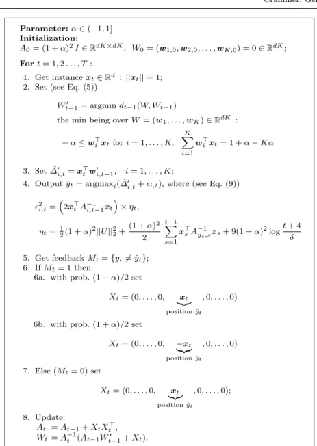
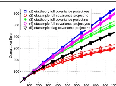
In order to illustrate the properties of the three abovementioned imple-mentation choices for Confidit(full vs diagonal matrices, projection vs. no projection, theoretical vs. simplified confidence intervals), and to motivate our subsequent setting on the real-world data, we run a simple simulated experi-ment on synthetic data. Our goal is to underscore the contribution of each to the final performance. We ran five versions ofConfidit, ranging from ”theo-retical” to ”practical”. These are summarized in the following table.

Version Projection Upper conf.2_i,t Covariance Comment

1 yes (9) Full Algorithm 1

2 no (11) Full

3 no (9) Full

4 yes (11) Full

5 no (11) Diagonal Used in subsequent

experiments

We repeated the following experiment 10 times, the reported results be-ing an average over the 10 runs. On each run we generated 1,000 random examples of dimension 9, where the first 5 features were used to generate labels, and the remaining 4 features are random with zero mean and unit standrad deviation, with no correlation with other features or labels. One of five labels (this is a multiclass problem with K = 5) were generated using five (random) linear modelsui of dimension five through the first 5 features.

Specifically, a given instance vectorx = (x1, . . . , x9) is associated with class

i= arg maxj=1...5(uj,0,0,0,0)>x. The norm of the modelsui was recorded,

since Eq. (9) depends on it. Notice that these data are not generated according to model (2), thereby making the setting ofαinConfidit(and the associated projection step) lose much of its significance. In fact, in all cases we setα= 1, turningConfiditinto a deterministic algorithm.

We ran each of the five versions seven times. When (9) was used (variants 1 and 3) we setkUkto be the squared norm of the model used to generated the data, scaled by one of the 7 values 10−3_,₁₀−2_{, . . . ,}₁₀3_{, which were meant} to provide a further “knob” to Eq. (9), possibly capturing the variability due to the confidence levelδ therein. Otherwise, when (11) was used (variants 2, 4 and 5), we setη= 10−3_,₁₀−2_{, . . . ,}₁₀3_{, seven values all together.}

The results are summarized in Fig. 2 showing the (average) cumulative number of mistakes for each of the five variants and the seven choices of pa-rameters. Interestingly, Algorithm 1 (shown in blue squares) performs worst, with more than 600 mistakes after 1,000 examples. The version that uses (11)

(18)

100 200 300 400 500 600 700 800 900 1000 100 200 300 400 500 600 Example index Cumulative Error

(1) eta:theory full covariance project:yes (2) eta:simple full covariance project:no (3) eta:theory full covariance project:no (4) eta:simple full covariance project:yes (5) eta:simple diag covariance project:no

Fig. 2 Averaged (over ten random generations of data) cumulative number of mistakes for

each of the five variants and seven choices of parameters.

rather than (9) (magenta diamonds) performs slightly better, with slightly less than 600 mistakes. The versions with no projection perform better, where the one that uses (9) (green stars) makes about 500 mistakes and the one that uses (11) (red circles) performing best, with about 300 mistakes. If we use diagonal matrices rather than full ones (black triangles), the performance drops and the number of mistakes increases to about 400. This fifth version is the one we used in our subsequent experiments, since it is much faster than all other (full matrix) versions.

In summary, these simple findings suggest that indeed the projection step

in Confidit is only needed for technical purposes related to the specifics of

our noise model, and that the confidence intervals computed by theory in (9) are too pessimistic. It seems that the full matrix version performs best, yet it is unfortunate that in many real-world problems it is not feasible to manipulate such matrices. It is also important to observe that performance is robust to the specific choice of parameters, as in most variants the total number of mistakes is within a range of about 30.

The three Confidit’s competitors that work in the full information set-ting are the classical Perceptron algorithm (Rosenblatt, 1958) extended to the multiclass setting as by Crammer and Singer (2003), a diagonal multiclass version of the 2nd-order perceptron algorithm (Cesa-Bianchi et al, 2005), and AROW (Crammer et al, 2009b). Note that only AROW is margin-based among all five algorithms. All other algorithms are mistake driven (at most). This dif-ference will be reflected in the performance of the algorithms.

(19)

In all experiments with real-world data we performed 10-fold cross valida-tion for all algorithms. Algorithm’s parameters (γfor Banditron,rfor AROW,

η forConfiditandafor the 2nd order Perceptron) were tuned using a single

split of the data into 80% training and 20% evaluation. In a preliminary set of experiments we also evaluated the influence of the parameterαforConfidit. Since the optimal value was very close to 1 anyway, with no significant im-provement in the results, we decided to set8 _α _{= 1 even on the real-world} datasets.

6 Empirical Results

We now report our results on real-world datasets, starting from text catego-rization. We summarize these results both in terms of cumulative number of mistakes in the online setting and in terms of test error in the batch setting, beginning with the former.

6.1 Online Results for Text Categorization

Evaluation of all algorithms in the online setting is split into Figure 3 and Fig-ure 4. We refer to the best scoring label (prediction) as ˜yt= arg maxiw>i,t−1xt,

and to the one actually output as ˆyt. For Perceptron, 2nd-order Perceptron and

AROW, these two are always the same. On the contrary, bandit algorithms work in the partial information setting, hence their need to make prediction ˜yt

and output label ˆytbe generally different. In particular, Banditron outputs a

uniformly random label with some fixed probability, whileConfiditoutputs the label with the highest sum of score and confidencew>_i,t₋₁xt+i,t.

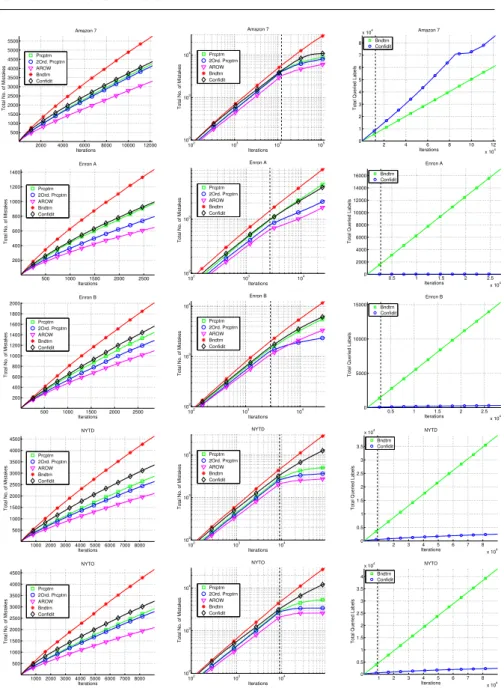
We refer now to Figure 3 which summarizes the results for four represen-tative datasets. Similar observations hold for the other five datasets shown in Figure 4. The left column of Figure 3 summarizes the cumulative number of

prediction mistakes each of the five online algorithms makes during its first

training epoch over the data. The plots are in a linear-linear scale. The four datasets are (top to bottom): 20 newsgroups, Amazon3, NYTS, and Reuters. We observe that AROW makes the least number of mistakes, while Banditron makes the most. There is no clear ordering between the other algorithms. This is surprising since Confidithas only partial information, on each iteration, while Perceptron and 2nd-order Perceptron do rely on full label information. Furthermore, we expected algorithms that employ (diagonal) 2nd-order infor-mation (e.g., 2nd-order Perceptron), to outperform algorithms that are based only on first order information (e.g., Perceptron).

8 _{Recall that}_α_{quantifies our prior knowledge about the amount of overlap among the}_K

classes. This prior knowledge is enforced through the projection step inConfidit. Since we decided to remove the projection from our implementation, the role ofαindeed loses much of its practical significance.

(20)

2000400060008000 10000 12000 14000 16000 2000 4000 6000 8000 10000 12000 14000 Iterations

Total No. of Mistakes

20 News Prcptrn 2Ord. Prcptrn AROW Bndtrn Confidit 102 103 104 105 102 103 104 105 Iterations

20 News Prcptrn 2Ord. Prcptrn AROW Bndtrn Confidit 2 4 6 8 10 12 14 16 x 104 0 0.5 1 1.5 2 2.5 3 3.5 4 4.5 x 104 Iterations

Total Queried Labels

20 News Bndtrn Confidit 0.5 1 1.5 2 2.5 3 x 104 500 1000 1500 2000 2500 3000 3500 4000 Iterations

Amazon 3 Prcptrn 2Ord. Prcptrn AROW Bndtrn Confidit 102 103 104 105 102 103 104 Iterations

Amazon 3 Prcptrn 2Ord. Prcptrn AROW Bndtrn Confidit 0.5 1 1.5 2 2.5 3 x 105 0 2 4 6 8 10 12 14 16 x 104 Iterations

Amazon 3 Bndtrn Confidit 1000 2000 3000 4000 5000 6000 7000 8000 500 1000 1500 2000 2500 3000 3500 4000 4500 5000 5500 Iterations

NYTS Prcptrn 2Ord. Prcptrn AROW Bndtrn Confidit 102 103 104 102 103 104 Iterations

NYTS Prcptrn 2Ord. Prcptrn AROW Bndtrn Confidit 1 2 3 4 5 6 7 8 x 104 0 0.5 1 1.5 2 2.5 3 3.5 4 x 104 Iterations

NYTS Bndtrn Confidit 1 2 3 4 5 6 x 105 0.5 1 1.5 2 2.5 3 3.5 4 x 104 Iterations

Reuters Prcptrn 2Ord. Prcptrn AROW Bndtrn Confidit 102 103 104 105 106 102 103 104 105 Iterations

Reuters Prcptrn 2Ord. Prcptrn AROW Bndtrn Confidit 1 2 3 4 5 6 x 106 0 2 4 6 8 10 12 14 x 105 Iterations

Reuters Bndtrn Confidit

Fig. 3 Cumulative number of prediction mistakes in the first training epoch (left;

linear-linear scale), and in all 10 epochs (middle; log-log scale), no label noise. The right plots shows the cumulative number of examples for which a prediction ˆyof a bandit algorithm is

notthe label output ˜y. Four datasets are used (top to bottom): 20 newsgroups, Amazon3, NYTS and Reuters.

The second column of Figure 3 summarizes the cumulative number of

pre-dictionmistakes overtentraining epochs over the data. The plots are in a

log-log scale. The vertical dashed black line indicates the end of the first epoch. In general, we observe a trend similar to the one observed after the first epoch. Banditron makes the same rate of mistakes in later epochs as the first one, yet it is not always the case for the other algorithms. For example, on 20 newsgroups (top plots) all other algorithms make noticeably fewer mistakes in the last 9 training epochs (on average) compared to the number of mistakes they make in the first iteration. The parameters of all algorithms were the

(21)

2000 4000 6000 8000 10000 12000 500 1000 1500 2000 2500 3000 3500 4000 4500 5000 5500 Iterations

Amazon 7 Prcptrn 2Ord. Prcptrn AROW Bndtrn Confidit 2 4 6 8 10 12 x 104 0 1 2 3 4 5 6 7 8 x 104 Iterations

Amazon 7 Bndtrn Confidit 500 1000 1500 2000 2500 200 400 600 800 1000 1200 1400 Iterations

Enron A Prcptrn 2Ord. Prcptrn AROW Bndtrn Confidit 102 103 104 102 103 Iterations

Enron A Prcptrn 2Ord. Prcptrn AROW Bndtrn Confidit 0.5 1 1.5 2 2.5 x 104 0 2000 4000 6000 8000 10000 12000 14000 16000 Iterations

Enron A Bndtrn Confidit 500 1000 1500 2000 2500 200 400 600 800 1000 1200 1400 1600 1800 2000 Iterations

Enron B Prcptrn 2Ord. Prcptrn AROW Bndtrn Confidit 102 103 104 102 103 104 Iterations

Enron B Prcptrn 2Ord. Prcptrn AROW Bndtrn Confidit 0.5 1 1.5 2 2.5 x 104 0 5000 10000 15000 Iterations

Enron B Bndtrn Confidit 1000 2000 3000 4000 5000 6000 7000 8000 500 1000 1500 2000 2500 3000 3500 4000 4500 Iterations

NYTD Prcptrn 2Ord. Prcptrn AROW Bndtrn Confidit 102 103 104 102 103 104 Iterations

NYTD Prcptrn 2Ord. Prcptrn AROW Bndtrn Confidit 1 2 3 4 5 6 7 8 x 104 0 0.5 1 1.5 2 2.5 3 3.5 x 104 Iterations

NYTD Bndtrn Confidit 1000 2000 3000 4000 5000 6000 7000 8000 500 1000 1500 2000 2500 3000 3500 4000 4500 Iterations

NYTO Prcptrn 2Ord. Prcptrn AROW Bndtrn Confidit 102 103 104 102 103 104 Iterations

NYTO Prcptrn 2Ord. Prcptrn AROW Bndtrn Confidit 1 2 3 4 5 6 7 8 x 104 0 0.5 1 1.5 2 2.5 3 3.5 4 x 104 Iterations

NYTO Bndtrn Confidit

Fig. 4 Same as Figure 3, with the remaining five datasets (top to bottom): Amazon7, Enron

A, Enron B, NYTD, and NYDO.

ones that minimize the error on held-out-data, which may be far from optimal when evaluating just on the number of online mistakes.

Finally, the right column of Fig. 3 summarizes the cumulative number of examples for which the prediction and the output of bandit-based algorithms

(22)

are not the same. This may be thought of as anexploration rateortotal queried

labels - which is the total number of time for which the algorithm output a

label which is not the best according to the model. Clearly, this only applies to Banditron and Confidit. The plots are in linear-linear scale. By definition, Banditron has afixed exploration rate (ofγ), as opposed to Confiditwhose exploration rate varies as more examples are observed. In seven out of the nine datasets (four are plotted in Figure 3, the other five are in Figure 4)Confidit

haslowerand monotonically decreasing exploration rate.Confidithas more

cumulative exploration rate in two of the datasets: Amazon3 and Amazon7. A possible explanation is that the number of features in these datasets is large (the largest among the nine datasets). Since the exploration rate ofConfidit

is based on a term which is linear in the square of the features, and there are many rare features, new features are introduced at a high-rate during training. As a result,Confiditgets biased towards exploring classes with a high number of relatively rare features.

6.2 Batch Evaluation for Text Categorization

Table 2 summarizes averaged 10-fold cross-validation error rates. Bold entries indicate best results within all algorithms except AROW (which is margin based), while underlined entries indicate superiority when comparing only the two bandit-based algorithms Banditron andConfidit. It is not surprising that AROW outperforms all other algorithms, as it works in the full information case with a margin-sensitive update rule. (This was shown for the binary case by Crammer et al (2009b)). Thus we consider below only Perceptron and 2nd-order Perceptron in the full information setting, and their bandit counterparts: Banditron and Confidit. When comparing the two algorithms working in the full information setting, we see that 2nd-order Perceptron outperforms Perceptron in 6 datasets, and is worse in 2 (there is a tie on one dataset). In fact the 2nd-order Perceptron outperforms all other three algorithms in 4 datasets. Confidit performs best among all four algorithms (including full information ones) in three datasets, and outpeforms Banditron in all dataset. All results, except one, are statistically significant with p-value of 0.001.

6.3 Label Noise for Text Categorization

We repeated the above experiments with artificial label noise injected into the training data. Specifically, we picked examples from the training set with probability p, and replaced the true label of these examples with a uniformly distributed random label. This process was performed only for the training subset of the data, the test results were evaluated using uncorrupted data. However, parameter tuning was performed using only corrupted data. The motivation here is that injecting label noise might be more harmful in the bandit setting than the full information setting. This is because the bandit

(23)

Second Order

Task Perceptron Perceptron AROW Banditron Confidit

20 newsgroups 20.04 13.92 8.14 50.52 ?12.41 Amazon7 25.71 25.73 22.30 29.15 (?)24.73 Amazon3 5.52 5.45 4.47 7.54 (?)6.67 Enron A 21.39 19.57 16.39 27.35 (?)23.01 Enron B 34.02 33.32 27.11 42.49 (?)37.89 NYTD 22.02 20.95 17.61 31.23 (?)27.02 NYTO 21.84 22.69 17.20 31.64 (?)25.20 NYTS 49.16 51.23 43.05 56.06 (†)54.24 Reuters 4.29 3.96 2.92 4.59 ?3.55

Table 2 Test error with 10-fold cross validation with no label noise. Bold entries indicate

lowest error-rate among the Perceptron, 2nd order Perceptron, Banditron and Confidit algo-rithms (AROW is not included, since it is margin-based, unlike the others), and underlined entries indicates lowest error-rate between the two bandit algorithms. Additional†and ?

indicate p-value of 0.01 and 0.001 respectively, when comparing all results, while (†) and (?) only include comparison between the two bandit-based algorithms.

Second Order

20 newsgroups 31.27 22.03 13.10 53.04 ?17.70 Amazon7 30.96 31.53 23.46 34.74 †29.49 Amazon3 12.51 12.17 5.42 16.12 ?8.90 Enron A 32.52 27.65 19.73 36.85 (?)27.58 Enron B 41.14 40.64 34.05 46.15 (?)41.27 NYTD 28.46 28.15 19.57 37.60 (?)28.94 NYTO 29.35 27.66 20.14 39.00 (?)27.87 NYTS 53.31 54.55 44.26 58.22 (?)54.82 Reuters 16.79 16.86 3.64 18.92 ?5.96

Table 3 Same as Table 2, with 10% training label noise.

Second Order

20 newsgroups 38.33 30.54 18.49 67.38 ?23.67 Amazon7 35.49 41.63 25.02 39.46 ?32.80 Amazon3 20.04 19.34 6.94 23.80 ?11.29 Enron A 38.77 36.62 22.75 43.15 ?29.40 Enron B 50.48 46.50 36.63 54.89 ?45.14 NYTD 36.90 34.92 21.46 43.99 ?31.63 NYTO 35.62 34.26 21.81 45.17 ?31.16 NYTS 59.42 57.69 46.82 61.77 ?54.90 Reuters 25.94 26.46 4.03 28.77 ?8.58

algorithms not only observe partial information, but when they get some, this information may be incorrect.

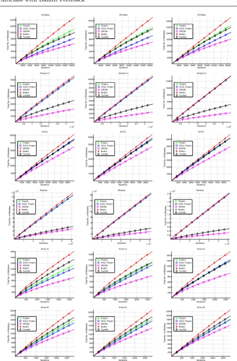
Online results for six datasets are given in three groups of plots. Figure 5 shows the cumulative number of mistakes (compared to the true non-corrupted label) for three noise levels: 10%, 20%, and 30% (left to right), similar to the

(24)

Second Order

20 newsgroups 45.88 39.92 21.41 65.71 ?30.45 Amazon7 42.33 41.41 27.47 45.28 ?36.24 Amazon3 28.70 27.38 6.22 31.70 ?17.16 Enron A 46.85 46.09 24.04 49.20 ?33.01 Enron B 55.52 54.89 37.17 61.10 ?50.57 NYTD 43.14 43.36 24.40 50.74 ?34.93 NYTO 44.43 42.40 24.78 48.85 ?33.85 NYTS 63.39 63.66 48.99 65.63 ?55.84 Reuters 35.34 35.70 4.53 36.61 ?11.70

left column of Figure 3. Figure 6 shows the cumulative number of mistakes (compared to the true non-corrupted label) on 10 training epochs for the three noise levels:0% (no noise),920%, and 30% (left to right), to be compared to the middle column of Figure 3. Finally, Figure 7 shows the cumulative number of examples for which the prediction and the output of bandit-based algorithms are not the same for the three noise levels: 10%, 20% and 30% (left to right), similar to the right column of Figure 3. As before, this may be thought of as

anexploration rate, and it only applies to Banditron andConfidit.

Comparing the three columns of Figure 5 per row, we observe that all algorithms make more mistakes, still the relative ordering remains the same. For example, the 2nd-order Perceptron algorithm makes about 8,000 mistakes on the 20 newsgroups data set of which 10% of the labels were corrupted, about 9,000 mistakes when 20% of the labels were corrupted, and about 10,000 mistakes when 30% of the labels were corrupted. Similar trend is observed for

Confiditwhich makes about 10,000, 11,500 and 12,000 mistakes when run

on the same data corrupted with 10%, 20% and 30% label-noise, respectively. Comparing the three columns of Figure 6 per row, we observe that, when run on noisy data (second and third columns), all algorithms continue to make mistakes after the first epoch at a rate that remains similar throughout time. This is in contrast to the evidence we collected on noiseless data (left column), where the mistake rate curves tend to flatten out in later epochs. The phe-nomenon was observed in the full information setting as well: Since the data are not separable the algorithms will continue to make mistakes.

Additionally, from Figure 7 we see that compared to the noise-free case,

Confidithas more exploration in some datasets, and comparable in others.

In these plots we show the total queried labels - the total number of time for which the algorithm output a label which is not the best according to the model. This is also due to the different value of exploration-exploitation parameter η automatically set by cross-validation. For example, in the first

9 _{The left column Figure 6 shows the results for 0% label noise, rather than 10%, as in}

Figure 5. This is because, after the first iteration the performance of most algorithms on noisy data has similar characteristics, as opposed to non-noisy data. However, on the first epoch the characteristics are changing gradually when we increase the label noise.

(25)

2000400060008000 10000 12000 14000 16000 2000 4000 6000 8000 10000 12000 14000 Iterations

20 News Prcptrn 2Ord. Prcptrn AROW Bndtrn Confidit 2000400060008000 10000 12000 14000 16000 2000 4000 6000 8000 10000 12000 14000 Iterations

20 News Prcptrn 2Ord. Prcptrn AROW Bndtrn Confidit 0.5 1 1.5 2 2.5 3 x 104 1000 2000 3000 4000 5000 6000 7000 Iterations

Amazon 3 Prcptrn 2Ord. Prcptrn AROW Bndtrn Confidit 0.5 1 1.5 2 2.5 3 x 104 1000 2000 3000 4000 5000 6000 7000 8000 9000 10000 Iterations

Amazon 3 Prcptrn 2Ord. Prcptrn AROW Bndtrn Confidit 0.5 1 1.5 2 2.5 3 x 104 2000 4000 6000 8000 10000 12000 Iterations

Amazon 3 Prcptrn 2Ord. Prcptrn AROW Bndtrn Confidit 1000 2000 3000 4000 5000 6000 7000 8000 1000 2000 3000 4000 5000 6000 Iterations

NYTS Prcptrn 2Ord. Prcptrn AROW Bndtrn Confidit 1000 2000 3000 4000 5000 6000 7000 8000 1000 2000 3000 4000 5000 6000 Iterations

NYTS Prcptrn 2Ord. Prcptrn AROW Bndtrn Confidit 1 2 3 4 5 6 x 105 1 2 3 4 5 6 7 8 9 10 11x 10 4 Iterations

Reuters Prcptrn 2Ord. Prcptrn AROW Bndtrn Confidit 1 2 3 4 5 6 x 105 2 4 6 8 10 12 14 16 x 104 Iterations

Reuters Prcptrn 2Ord. Prcptrn AROW Bndtrn Confidit 1 2 3 4 5 6 x 105 0.2 0.4 0.6 0.8 1 1.2 1.4 1.6 1.8 2 2.2 x 105 Iterations

Reuters Prcptrn 2Ord. Prcptrn AROW Bndtrn Confidit 500 1000 1500 2000 2500 200 400 600 800 1000 1200 1400 1600 Iterations

Enron A Prcptrn 2Ord. Prcptrn AROW Bndtrn Confidit 500 1000 1500 2000 2500 200 400 600 800 1000 1200 1400 1600 Iterations

Enron A Prcptrn 2Ord. Prcptrn AROW Bndtrn Confidit 500 1000 1500 2000 2500 200 400 600 800 1000 1200 1400 1600 1800 2000 Iterations

Enron B Prcptrn 2Ord. Prcptrn AROW Bndtrn Confidit 500 1000 1500 2000 2500 200 400 600 800 1000 1200 1400 1600 1800 2000 Iterations

Enron B Prcptrn 2Ord. Prcptrn AROW Bndtrn Confidit 500 1000 1500 2000 2500 200 400 600 800 1000 1200 1400 1600 1800 2000 2200 Iterations

Enron B Prcptrn 2Ord. Prcptrn AROW Bndtrn Confidit

Fig. 5 Cumulative number of prediction mistakes in the first training epoch in linear-linear

scale for three noise levels 10%, 20% and 30% (left to right). Six datasets are shown (top to bottom): 20 newsgroups, Amazon3, NYTS, Reuters, Enron A and Enron B.

(26)

102 103 104 105 102 103 104 105 Iterations

20 News Prcptrn 2Ord. Prcptrn AROW Bndtrn Confidit 102 103 104 105 102 103 104 Iterations

Amazon 3 Prcptrn 2Ord. Prcptrn AROW Bndtrn Confidit 102 103 104 105 102 103 104 105 Iterations

Amazon 3 Prcptrn 2Ord. Prcptrn AROW Bndtrn Confidit 102 103 104 102 103 104 Iterations

NYTS Prcptrn 2Ord. Prcptrn AROW Bndtrn Confidit 102 103 104 105 106 102 103 104 105 Iterations

Reuters Prcptrn 2Ord. Prcptrn AROW Bndtrn Confidit 102 103 104 105 106 102 103 104 105 106 Iterations

Reuters Prcptrn 2Ord. Prcptrn AROW Bndtrn Confidit 102 103 104 102 103 Iterations

Enron A Prcptrn 2Ord. Prcptrn AROW Bndtrn Confidit 102 103 104 102 103 104 Iterations

Enron B Prcptrn 2Ord. Prcptrn AROW Bndtrn Confidit

Fig. 6 Cumulative number of prediction mistakes in 10 training epochs in linear-linear

scale for three noise levels0%, 20% and 30% (left to right). Six datasets are shown (top to bottom): 20 newsgroups, Amazon3, NYTS, Reuters, Enron A and Enron B.

(27)

2 4 6 8 10 12 14 16 x 104 0 1 2 3 4 5 6 7 8x 10 4 Iterations

20 News Bndtrn Confidit 2 4 6 8 10 12 14 16 x 104 0 1 2 3 4 5 6 7 8 x 104 Iterations

20 News Bndtrn Confidit 2 4 6 8 10 12 14 16 x 104 0 1 2 3 4 5 x 104 Iterations

20 News Bndtrn Confidit 0.5 1 1.5 2 2.5 3 x 105 0 2 4 6 8 10 12 14 16 18 x 104 Iterations

Amazon 3 Bndtrn Confidit 0.5 1 1.5 2 2.5 3 x 105 0 5 10 15x 10 4 Iterations

Amazon 3 Bndtrn Confidit 0.5 1 1.5 2 2.5 3 x 105 0 2 4 6 8 10 12 x 104 Iterations

Amazon 3 Bndtrn Confidit 1 2 3 4 5 6 7 8 x 104 0 1 2 3 4 5 x 104 Iterations

NYTS Bndtrn Confidit 1 2 3 4 5 6 7 8 x 104 0 1 2 3 4 5 x 104 Iterations

NYTS Bndtrn Confidit 1 2 3 4 5 6 7 8 x 104 0 0.5 1 1.5 2 2.5 3 3.5 4 x 104 Iterations

NYTS Bndtrn Confidit 1 2 3 4 5 6 x 106 0.5 1 1.5 2 2.5 3 x 106 Iterations

Reuters Bndtrn Confidit 1 2 3 4 5 6 x 106 0.5 1 1.5 2 2.5 3 x 106 Iterations

Reuters Bndtrn Confidit 0.5 1 1.5 2 2.5 x 104 0 2000 4000 6000 8000 10000 12000 Iterations

Enron A Bndtrn Confidit 0.5 1 1.5 2 2.5 x 104 0 2000 4000 6000 8000 10000 12000 Iterations

Enron A Bndtrn Confidit 0.5 1 1.5 2 2.5 x 104 0 2000 4000 6000 8000 10000 12000 14000 16000 Iterations

Enron A Bndtrn Confidit 0.5 1 1.5 2 2.5 x 104 0 2000 4000 6000 8000 10000 12000 14000 Iterations

Enron B Bndtrn Confidit 0.5 1 1.5 2 2.5 x 104 0 2000 4000 6000 8000 10000 12000 Iterations

Enron B Bndtrn Confidit 0.5 1 1.5 2 2.5 x 104 0 1000 2000 3000 4000 5000 6000 7000 8000 Iterations

Enron B Bndtrn Confidit

Fig. 7 The cumulative number of examples for which a prediction ˆyof a bandit algorithm

isnotthe label output ˜yfor three noise levels 10%, 20% and 30% (left to right). Six datasets are shown (top to bottom): 20 newsgroups, Amazon3, NYTS, Reuters, Enron A and Enron B.

(28)

row of Figure 7 we see that for 20 newsgroup Confidit has about 20,000 queries altogether for 10% label noise, about 25,000 queries for 20% label noise, and about 40,000 queries for 30% label noise. This relation can also be observed on the EnronB dataset (last row). On other datasets, the trend is inverse (less queries with more noise, e.g., EnronA, 2nd line form the bottom), and on others there is no clear trend.

Finally, averaged 10-fold cross validation error rates on label noise rates 10% 20%, and 30% are summarized in Table 3, Table 4 and Table 5, respec-tively. Evaluations are performed using uncorrupted data, the noisy data being used only during training and parameter tuning. There are few trends. First, as expected, performance degrades as the level of noise increases. For example, on the Amazon7 dataset the error rate of Banditron increases from 29.15% via 34.74% via 39.46% to 45.28% as the label noise levels range from 0% (see Table 2) to 10% to 20% to 30%. Second, as the level of noise increases, it seems thatConfiditsuffers the least compared to Perceptron and 2nd-order Perceptron. For example, on Amazon3 both Perceptron and 2nd-order Per-ceptron have about 5.50% error when trained with no noise (Table 2), while having about 12% error with 10% label noise. Confidit, on the other hand, has 6.57% error with no noise, and about 8.90% with noise. Third, in fact, whileConfiditperforms best (among the four non margin-based algorithms) on only 3 datasets out of 9 when no noise is induced, it is the best in 4 datasets at a 10% label noise level, and is best on all 9 datasets for 20% and 30% noise. HenceConfiditseems more resilient to label noise compared to Banditron, as well as to the other two full information algorithms: Perceptron and 2nd-order Perceptron.

6.4 Batch Evaluation for Vowel Recognition

Following the experimental setting in Lin et al (2009), we now give batch evaluation results on the four vowel recognition datasets. Generally speaking, similar trends as those reported on the text categorization datasets can be observed.

Test test accuracies as a function of the training set size are contained in Figure 8. All online algorithms made a single pass over the training data. The figure also includes the test set accuracy of the Probabilistic Linear Machine (PLM) algorithm (Lin et al, 2009), which achieves state-of-the-art results for that task. The PLM algorithm was trained using the entire training set. The top row shows the results for the smaller set of four labels (“v4”), and the bottom one for the larger set of eight labels (“v8”). The left column summarizes the results for one feature window (“w1”), the right column is for the seven feature window (“w7”).

Focusing on the top-left panel we observe that PLM achieves 90.0% accu-racy. AROW andConfiditachieve an accuracy of 89% or higher using only 1,000 examples. AROW achieves PLM’s accuracy with about 2,000 training examples, and Confidit with about 20,000. The full training set size has