WORKING PAPER NO. 124
STOCK RETURN VOLATILITY PATTERNS IN INDIA
AMITA BATRA
Contents
Foreword ...i
Abstract ...ii
I Introduction ...1
II Theoretical Motivation...4
III Survey of Literature...6
IV Data...8
IV.1 Basic Data ...8
IV.2 Sample Period ...9
IV.3 Sources of Data ...9
IV.4 Descriptive Statistics...9
V Estimating Volatility: Exponential GARCH (E-GARCH)...10
VI The Analysis: Our Approach ...12
VI.1 Naïve Model...12
VI.2 Augmented GARCH Model ...16
VI.3 Characteristics of Stock Market Cycles ...22
VII Conclusions ...28
APPENDIX ...30
Foreword
Financial crises in the last decade have revealed that financial asset price volatility has the potential to undermine financial stability. Available empirical evidence indicates that financial stability is endangered more by sudden shifts in volatility rather than by a sustained increase in the level of volatility. Understanding volatility is therefore central to risk management in an economy.
This paper examines the time variation in volatility in the Indian stock market during 1979-2003. Using monthly data and asymmetric GARCH methodology augmented by structural change analysis the paper identifies sudden shifts in stock price volatility and the nature of events that cause these shifts in volatility. The paper also undertakes an analysis of the stock market cycles in India to see if the bull and bear phases of the market have exhibited greater volatility in recent times.
The empirical analysis in the paper reveals that the period around the BOP crisis and the subsequent initiation of economic reforms in India is the most volatile period in the stock market. Sudden shifts in stock return volatility in India are more likely to be a consequence of major policy changes and any further incremental policy changes may have only a benign influence on stock return volatility. Stock return volatility in India seems to be influenced more by domestic political and economic events rather than by global events. The analysis in the paper also reveals that stock market cycles in India have not intensified after financial liberalization. A generalized reduction in stock market instability is observed in the post reform period in India.
I do hope that this paper will serve as a useful source and provide valuable reference material for researchers, policymakers and market participants.
Arvind Virmani
Director & Chief Executive ICRIER March 2004
* Sincere thanks are offered to Prof. Arvind Virmani for giving invaluable suggestions that helped me finalize the paper. Thanks are due to an anonymous referee for making useful comments on the first draft. Thanks are also offered to Dr. Reena Aggarwal and Dr. Carla Inclan for giving the relevant econometric packages and to Mr. Vipul Bhatt for technical assistance. Research assistance provided by Ms. Zeba Khan is deeply appreciated.
STOCK RETURN VOLATILITY PATTERNS IN INDIA
Amita Batra*
Abstract
In this paper we analyze the time variation in volatility in the Indian stock market during 1979-2003. We examine if there has been an increase in volatility persistence in the Indian stock market on account of the process of financial liberalization in India. Further, we examine the shifts in stock price volatility and the nature of events that apparently cause the shifts in volatility. We also make an attempt to characterize the evolution of the stock market cycles over time in India and examine if in recent times the stock market cycles have exhibited greater amplitude and volatility. In an overall sense, therefore, the aim of this paper is to give economic significance to changes in the pattern of stock market volatility in India during 1979-2003.
Monthly stock returns have been used for analysis. Asymmetric GARCH model has been used to estimate the element of time variation in volatility. The model is further augmented with dummy variables, an outcome of the structural change analysis, to examine volatility persistence. For the characterization of the stock market cycles, the Pagan and Sussoumov (2003) methodology is adopted.
Our analysis reveals that the period around the BOP crisis and the initiation of economic reforms in India is the most volatile period in the stock market. Structural shifts in volatility are more likely to be a consequence of major policy changes and any further incremental policy changes may have only a benign influence on stock return volatility. Stock return volatility in India seems to be influenced more by the domestic political and economic events rather than global events. In particular there appears to be no coincidence between volatility of portfolio capital flows in and out of the stock market and the volatility shifts in stock returns in India. Our analysis also shows that stock market cycles in India have not intensified after financial liberalization. We observe a generalized reduction in market instability in the post reform period in India. In general, in the post liberalization period in India, the bull phases are longer, the amplitude of bull phases is higher and the volatility in bull phases is also higher than in the bear phases. In comparison with its pre liberalization character, however, the bull phases are more stable in the post liberalization period.
Key Words: Persistence of volatility shocks; structural change; stock market cycles
I Introduction
In the aftermath of the many crises that the last decade has been witness to, a return to the old- world order of regulated/restricted flows has been proposed by many economists and policymakers. The clamor for restrictions on capital inflows has largely been on account of the notion that unregulated cross – border movement of portfolio capital causes “excessive” booms and busts and thus volatility/instability in the financial markets. Financial market volatility can have a wide repercussion on the economy as a whole. There is clear evidence of the important link between financial market
uncertainty1 and public confidence. Policy makers therefore rely on market estimates of
volatility as a barometer of the vulnerability of financial markets. The existence of excessive volatility or “noise” also undermines the usefulness of stock prices as a “signal” about the true intrinsic value of a firm, a concept that is core to the paradigm of informational efficiency of markets. Further, volatility estimation and forecasting have become a compulsory risk –management exercise for economies and many financial institutions around the world ever since the first Basle Accord was established in 1996. Understanding volatility is therefore central to risk management in an economy.
In the asset pricing literature volatility refers to asset price variability. Volatility may be measured as the standard deviation of daily price changes, or as a by-product of estimation of an econometric volatility model. The standard approach to modeling volatility is through the so-called GARCH class of ARCH models. The availability of long series of asset price data has resulted in a large number of econometric studies on volatility. A general finding across asset markets is that volatility shocks are highly persistent.
1 When volatility is interpreted as uncertainty it becomes a key input into many investment decisions and
portfolio creations. Investors and portfolio managers have certain levels of risk, which they can bear. A good forecast of the volatility of asset prices over the investment holding period is a good starting point for assessing risk.
In this paper we analyze the time variation in volatility2 in the Indian stock market during 1979-2003. We examine if there has been an increase in volatility persistence in the Indian stock market on account of the process of financial3 liberalization in India. Further, we examine the shifts in stock price volatility and the nature of events that apparently cause the shifts in volatility. This will enable us to identify if a coincidence between the shifts in stock return volatility and financial liberalization exists. We also make an attempt to characterize the evolution of the stock market cycles over time in India and examine if in recent times the stock market cycles have exhibited greater amplitude and volatility. The analysis of bear and bull markets allows us to investigate in greater detail and in an episodic manner, the evolution of stock market instability. In an overall sense, therefore, the aim of this paper is to give economic significance to changes in the pattern of stock market volatility in India during 1979-2003.
Monthly stock returns have been used for analysis as the presence of more noise at higher frequencies makes it difficult to isolate cyclical variations, obscuring thus the analysis of the driving moments of switching behavior in stock price volatility. Asymmetric GARCH model has been used to estimate the element of time variation in volatility. The model is further augmented with dummy variables, an outcome of the structural change analysis, to examine volatility persistence. For the characterization of the stock market cycles, the Pagan and Sussoumov (2003) methodology is adopted.
Our analysis of sudden shifts in stock index volatility reveals that the period around the 1991 BOP crisis and the subsequent initiation of economic reforms in India is the most volatile period in the stock market. Structural shifts in volatility are more likely to be a consequence of major policy changes and any further incremental policy changes may have only a benign influence on stock return volatility. Further, stock return
2 Stock return/market volatility may not be increasing in recent years or before /after an event but there
may be variation in volatility over time
3 While we seek to analyze volatility changes as a consequence of stock market liberalization and
portfolio inflows, we refer to financial liberalization in the paper, as the period of reference encompasses a large number of economic reform measures simultaneously undertaken to open the domestic financial sector.
volatility in India is influenced more by the domestic political and economic events rather than global events. In particular there appears to be no coincidence between volatility of portfolio capital flows in and out of the stock market and the volatility shifts in stock returns in India.
Our analysis also shows that stock market cycles in India have not intensified after financial liberalization. We observe a generalized reduction in instability in the post reform period in India. Interestingly our findings are in line with the nature of evolution of financial cycles in other emerging markets. An informal analysis shows that external linkages of the Indian stock market seem non-existent prior to 1998. After October 1998, coincidence with financial cycles in the US is visible. Specifically for the peak observed in the year 2000 a coincidence of peaks across the US and the emerging markets is observed. In general, in the post liberalization period in India, the bull phases are longer, the amplitude of bull phases is higher and the volatility in bull phases is also higher than for the bear phases. In comparison with its pre liberalization character, however, the bull phases are more stable in the post liberalization period.
The rest of the paper is organized as follows: In section 2 we present the theoretical motivation for our analysis. Section 3 gives a brief review of literature on the subject. Section 4 lists the data and data sources used for the analysis in this paper. Some summary descriptive statistics for the stock returns over our reference period are also presented in this section. Section 5 explains the exponential GARCH methodology. The empirical analysis is presented in section 6. The empirical analysis is undertaken in three parts viz: time variation in volatility using the asymmetric GARCH (E-GARCH) methodology, augmented E-GARCH using dummy variables for structural change in stock return volatility and volatility analysis using the stock market cycles approach. Main conclusions of our analysis are summarized in section 7.
II Theoretical Motivation
Both volatility persistence and stock market cycle characterization are currently empirical phenomena without a theoretical explanation; some theoretical underpinnings of the link between stock market volatility and liberalization have however evolved. We discuss below the channels through which stock market liberalization may affect volatility. The discussion is based on the model proposed by Tauchen and Pitts (1983) and subsequently used by Kwan and Reyes (1997). The model relates stock price and volume traded in the speculative market with clear implications for liberalization and stock return volatility.
Assume that there are J active traders in the market. Within the day, the market passes through a sequence of distinct Walrasian equilibria. The movement from the (I-1)st to the ith equilibrium in a given day is caused by the arrival of new information to the market. The desired net position, Qij of trader j at the time of the ith equilibrium is
assumed to be a linear function of the following form:
Qij = a [P*ij – Pi] (j = 1,2…..J) (1)
Where
a > 0 = constant
P*ij = jth trader’s reservation price Pi = current market price
A positive value for Qij represents a desired long position in a contract while negative
value represents a desired short position. Equilibrium requires that the following holds true:
Ê
jJ1 Qij = 0 (2)This implies that the average of the reservation price clears the market:
Pi =1/J
Ê
J j 1
The price change can then be written as:
DP = 1/J
Ê
Jj 1
D P*ij (4)
Where P*ij = P*ij-P*I-1, j is the increment to the jth trader’s reservation price. Assuming a variance – components model with an information component that is common to all traders, ji, and one that is specific to the jth trader, yij
Equation (4) can then be re - written as:
DPi = fI +1/J
Ê
J j 1
jij (5)
The first two moments of the price change are then derived as the following:
E[DPi] = 0 (6)
Var[D p i] = s2
+ s2/J (7)
Equation (7) suggests that other things being equal, an increase in the number of traders J tends to reduce the stock price variance. On the other hand, an increase in the variance of information sets available to traders – a common component and/or a unique component - tends to raise the stock price variance.
Stock market liberalization will attract a new group of investors, the FIIs. An increase in the number of traders in the market may then reduce the stock price variance. Stock market opening may also simultaneously trigger an increase in the variance of information sets available to the FII thereby implying a possibility of an increase in the stock return volatility. Theoretical literature therefore does not provide us with an unambiguous conclusion on the impact of stock market liberalization on stock return volatility.
III Survey of Literature
Most recent studies on financial market volatility are placed in the context of transmission of volatility across economies and the contagion effects of a financial crisis. These include studies by Forbes and Rigobon (2002), Bekaert, Harvey and Lumsdaine (2002a,b), Edwards (2000) and others. Rogobon (2003) has focussed on alternative measures of volatility in the equity and bond markets in the period surrounding the financial crises. Bekaert and Harvey (2000) analyzed equity returns in a group of emerging markets before and after financial reforms. The empirical studies investigating the volatility of returns have yielded mixed conclusions. Aggarwal, Inclan and Leal (1999) analyze volatility in emerging stock markets during 1985-95. Using an ICSS algorithm to identify the points of sudden changes in the variance of returns they examine the nature of events that cause large shifts in stock return volatility in these economies. Aggarwal et al find that mostly local events cause jumps in the stock market volatility of the emerging markets. Kim and Singal (1997) and De Santis and Imorohoroglu (1994) study the behavior of stock prices following the opening of a stock market to foreigners or large foreign inflows. They find that there is no systematic effect of liberalization on stock market volatility. These findings corroborate Bekaert’s findings that volatility in emerging markets is unrelated to his measure of market integration. Richards (1996) used three different methodologies and two sets of data to estimate volatility of emerging markets. A common claim of all these studies is that, the proposition that liberalization increases volatility is not supported by empirical evidence. However, Levine and Zervos (1995) suggest that volatility may increase after liberalization.
Hamao and Mei (2001) examined the impact of foreign and domestic trading on market volatility for Japan and find no systematic evidence that foreign trading tends to increase market volatility more than trading by domestic groups. The study however relates to the time period during which the foreign portfolio investment in Japan was rather small. Folkerts – Landau and Ito (1995) computed volatility of emerging markets in periods that differ in their intensity of portfolio flows. Their evidence is rather mixed
with Mexican stock prices being least volatile when flows are most volatile and vice versa for Hong Kong. Nilsson (2002) has explored that stock market liberalization can lead to excess volatility possibly on account of noise trading for Nordic stock markets using the Markov regime-switching model. He finds evidence of higher expected return, higher volatility and stronger links with international stock markets characteristic of the deregulated period in all Nordic stock markets.
Studies analyzing the behavior of stock prices over financial cycles have been undertaken in the recent years. They show that stock markets when liberalized tend to become more stable. Kaminsky and Schumkler (2001,2002) examine the time varying patterns of financial cycles before and after financial liberalization in 28 countries. Their results indicate that while financial liberalization may trigger financial excesses in the short-run it also triggers changes in institutions supporting a better functioning of financial markets. They observe a temporary volatility increase in the years immediately following liberalization in these countries. Edwards et al (2003) analyze the behavior of stock prices in six emerging countries. They find that after financial liberalization Latin American markets are less unstable while the Asian economies, especially Korea, are in the process of recovering their stability.
As is evident from the survey of literature discussed above, the issue of changes in volatility of stock returns on account of stock market liberalization in emerging markets has received considerable attention in recent years. However almost all the studies undertaken thus far analyze the changes in volatility across selected emerging markets in Latin America and East Asia. In most studies India is not included in the sample of countries for which liberalization and volatility is analyzed. We hope to fill this gap through our analysis.
In addition, in most studies a narrowly defined concept of financial liberalization is adopted. The date for a single event characterizing the opening of one of the financial markets is generally taken as the reference date for liberalization. We have tried to
overcome this by taking the reverse route of first looking at the structural breaks in stock return variance and then identifying the events to see if the break from the past behavior can at all be ascribed to a particular event or process of liberalization in the stock market.
IV Data
IV.1 Basic Data
We have used two stock market indices –the BSE sensex and the International Finance Corporation (and S&P) published IFC Global (IFCG) index. Sensex was a natural choice for our analysis, as it is the most popular market index4 and widely used by market participants for benchmarking. Also, existence of data for a longer period for the sensex is an added advantage. Sensex based stock returns are therefore the mainstay of the paper. US dollar returns as in the IFCG index are also used for analysis. Local currency returns enable us to analyze the impact on stock return volatility from a local perspective and the dollar returns give us a comparative foreign perspective.
Data have been used at monthly and daily frequency. However observed data at high frequency are often polluted by “ noise” . “ Noise” plays a key role in the high frequency volatility persistence. At less frequent observation, the “ noise” dies away. Monthly data is therefore the mainstay of this paper. The daily closing prices of the sensex are used as the source data to arrive at the monthly data. Days when there is no trading are omitted and the price change is calculated from the last day the market was open.
Returns are proxied by the log difference change in the price index.
Rt = log Pt – log Pt-1
Rt = return at time t
Pt, Pt-1 = closing value of the stock price index at time t, t-1.
4 Nifty is another popular index based on a 50 firm portfolio. However as the data is available only from
Even though Rt more accurately corresponds to capital gains we refer to these as
returns in accordance with the approach followed by parallel studies. The IFCG however represents total returns5.
IV.2 Sample Period6
Time period for sensex: 1979:04 – 2003:03 Time period for IFCG: 1988:01- 2001:12 IV.3 Sources of Data
Original data -published and unpublished, from official sources such as Securities and Exchange Board of India (SEBI), Reserve Bank of India and Bombay Stock Exchange (BSE) has been used. The data for stock price index for the period prior to 1991 is not available in a published form. Hence this has been procured from the relevant official records. Data on dollar returns has been culled from several issues of the emerging market database factbook published by the IFC. Data sources for other variables are several issues of the IFS (IMF), RBI monthly Bulletin and the Handbook of Statistics on the Indian Economy.
IV.4 Descriptive Statistics
Table IV.1 below gives a summary of the basic statistics relating to the sensex based stock returns in India.
5 This can contribute to difference in results with those obtained using IFC returns data. The IFC dollar
returns are inclusive of dividends and take into account stock splits and capital gains.
6 The lack of uniformity in the sample period for the two indices poses a limitation for our analysis. We
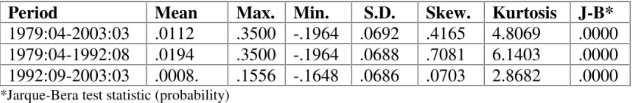
Table IV. 1 Summary Statistics for Sensex based Stock Returns in India7.
Period Mean Max. Min. S.D. Skew. Kurtosis J-B*
1979:04-2003:03 .0112 .3500 -.1964 .0692 .4165 4.8069 .0000
1979:04-1992:08 .0194 .3500 -.1964 .0688 .7081 6.1403 .0000
1992:09-2003:03 .0008. .1556 -.1648 .0686 .0703 2.8682 .0000
*Jarque-Bera test statistic (probability)
Mean returns are higher for the pre – liberalization period. There is in fact a large fall in the mean returns in India in the post liberalization period when compared with the pre liberalization phase. The standard deviation in returns, which is indicative of the unconditional variance in returns, however continues to remain almost the same in the two sub-periods. The return – risk trade-off as indicated by the Sharpe ratio in financial theory therefore shows a fall in the post liberalization period simply on account of the decrease in returns.
From the statistics we may also infer that the stock returns in India are unlikely to have been drawn from a normal distribution. The returns are skewed positively for the full sample period and in the pre liberalization period individually. The kurtosis statistic indicates that the returns are consistently leptokurtic. Furthermore, the Jarque-Bera statistic that tests the hypothesis of normal distribution is rejected at a very high level. For the post liberalization period however a non-normal distribution is not so certain.
V Estimating Volatility: Exponential GARCH (E-GARCH)
Stock return volatility is estimated using asymmetric GARCH (E-GARCH) methodology8. As indicated by the summary statistics presented in section five of this paper, the stock returns in India do not follow a normal distribution. Asymmetric E-GARCH model that allows for leptokurtosis and skewness is therefore considered
7 Based on monthly data.
8 Most earlier studies have used ARCH-GARCH model to estimate volatility of stock returns. However
as the stock returns in emerging markets are not generally drawn from a normal distribution asymmetric GARCH methodology is more appropriate.
appropriate to estimate volatility. The model can in addition capture the leverage and volatility clustering effects.
Under the E-GARCH methodology two distinct specifications for mean and variance are made. These are as follows:
Mean specification:
In the first step we specify the conditional mean equation for returns as:
Yt = m+ et………(1)
Variance specification:
In the second step we identify the conditional variance equation for returns. The
general specification of the conditional variance in the E-GARCH (p, q) model is as follows: 1 1 1 1 2 1 2) log( ) log( + + + = t t t t t t s e b s e g s a w s … … … .(2)
In this model specification a is the GARCH term that measures the impact of last period’s forecast variance. A positive a indicates volatility clustering implying that positive stock price changes are associated with further positive changes and vice versa.
g is the ARCH term that measures the effect of news about volatility from the previous
period on current period volatility. b measures the leverage effect. Ideally b is expected to be negative implying that bad news has a bigger impact on volatility than good news of the same magnitude. The sum of the ARCH-GARCH coefficients indicates the extent to which a volatility shock is persistent over time. A persistent volatility shock raises the asset price volatility.
VI The Analysis: Our Approach
Our analysis for volatility patterns of stock returns in India is undertaken in three stages as follows:
VI.1 Naïve Model
As a direct outcome of the Tauchen and Pitts model as specified in section 2, we examine if stock market liberalization and the consequent increase in the number of traders (the FIIs) leads to an increase in stock return volatility. We undertake a comparative analysis of the stock return volatility pre and post the entry of FIIs in the Indian stock market. For FII entry we specify three different dates corresponding to the Budget announcement (1992:02), actual policy announcement (1992:09) allowing FIIs to invest and the actual entry of FII that is the month when FIIs first invested in the Indian stock market (1992:11).
Results:
Results using both daily and monthly frequency9 are presented in the Tables VI.1 and
VI.2 respectively:
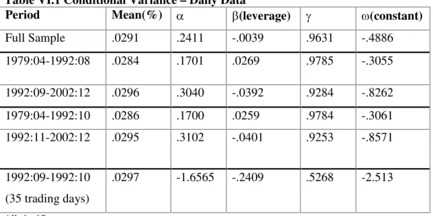
Table VI.1 Conditional Variance – Daily Data
Period Mean(%) a b(leverage) g w(constant)
Full Sample .0291 .2411 -.0039 .9631 -.4886 1979:04-1992:08 .0284 .1701 .0269 .9785 -.3055 1992:09-2002:12 .0296 .3040 -.0392 .9284 -.8262 1979:04-1992:10 .0286 .1700 .0259 .9784 -.3061 1992:11-2002:12 .0295 .3102 -.0401 .9253 -.8571 1992:09-1992:10 (35 trading days) .0297 -1.6565 -.2409 .5268 -2.513 All significant
9 However as has been indicated in the introduction, observed data at high frequency are often polluted
by “ noise” . “ Noise” plays a key role in the high frequency volatility persistence. At less frequent observation, the “ noise” dies away. For the rest of the paper therefore we proceed with monthly data.
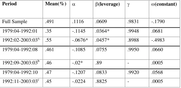
Table VI.2. Conditional Variance –Monthly Data
Period Mean(%) a b(leverage) g w(constant)
Full Sample .491 .1116 .0609 .9831 -.1790 1979:04-1992:01 .35 -.1145 .0364* .9948 .0681 1992:02-2003:03a, .55 -.0676* .0457* .8988 -.4983 1979:04-1992:08 .461 -.1085 .0755 .9950 .0660 1992:09-2003:03b .46 -.02* .89 - .0005 1979:04-1992:10 .47 -.1207 .0833 .9920 .0568 1992:11-2003:03c .45 -.0224 .8825 - .0005 *: Not significant
a: post liberalization w.r.t Budget EGARCH (1,1) model, b: w.r.t Actual announcement-GARCH(1,1) model and c: w.r.t Actual FII entry-announcement-GARCH(1,1) model.
The important feature of volatility that emerges from the above analysis is that the stock return data in India reveals high volatility persistence for both daily and monthly data and this remains almost unaltered throughout the sample period. The stock return series are exploding and very little change is evident in the pattern of volatility persistence between pre and post liberalization periods. The post liberalization period shows some fall in the persistence character of the stock return volatility for monthly data but the magnitude of fall is small and persistence continues to remain very high even in the post liberalization period.
As regards the level of volatility, mean volatility shows a slight increase in the post liberalization period for daily data even though the increase is marginal. This holds true for all the possible break dates (i.e. budget announcement, actual policy announcement and actual entry) regarding FII entry in the Indian stock market.
The results based on daily stock returns also indicate significant leverage in the Indian stock market full sample and in the post liberalization period. Leverage is however not indicated in the monthly data.
For monthly data volatility persistence is significantly evident for the full sample and also for the sub periods. The stock return volatility is observed to be explosive as throughout the sum of all the coefficients is greater than .85. Pre liberalization the sum is greater than 1 and this falls to .87 in the post liberalization period. The results are almost similar for the other break date (i.e. with FII entry date: 1992:11). The mean level of volatility does not change much throughout our sample period. A significant change is however observed when we consider the break date to be the budget date. While volatility persistence continues to be highly significant, the results also clearly indicate that the period between the budget of 1992 i.e. February 1992 and the actual policy announcement, September 1992, was a period of high volatility. Very high volatility change is observed if the break date is the budget date, while volatility remains constant with the break date as actual policy announcement and then falls if the break date relates to the actual entry of FIIs. From these results it may be possible to infer that it is the initial policy announcement that has the maximum impact on stock return volatility. Visual evidence to this effect may be gleaned from the following graphs:
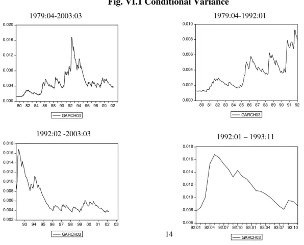
Fig. VI.1 Conditional Variance
0.000 0.004 0.008 0.012 0.016 0.020 80 82 84 86 88 90 92 94 96 98 00 02 GARCH03 1979:04-2003:03 0.000 0.002 0.004 0.006 0.008 0.010 80 81 82 83 84 85 86 87 88 89 90 91 92 GARCH03 1979:04-1992:01 0.002 0.004 0.006 0.008 0.010 0.012 0.014 0.016 0.018 1992:02 -2003:03 0.006 0.008 0.010 0.012 0.014 0.016 0.018 1992:01 – 1993:11
The above graphs show that the increase in volatility occurs during the intervening period of the first announcement towards a liberalized environment for foreign investors in the budget of 1992 and the final policy announcement effective September 1992.
The budget announcement towards allowing FII entry was however coupled with a number of other announcements towards economic reforms in India after the 1991 BOP crisis10. On the basis of the above results therefore it is difficult to ascribe the high persistence or the high level of stock return volatility only to the announcement effect of FII entry. Further, recent evidence on volatility in emerging markets suggests that the typically observed very high persistence as implied by the conventional GARCH model does not characterize the behavior of stock returns. In particular it has been shown that the typical GARCH model can exaggerate volatility persistence compared to the true volatility process perceived by the market11. This discrepancy is particularly pronounced
in cases where there are extreme shocks12. As our sample period covers a broad range of economic liberalization events it is possible that the volatility persistence could be a consequence of parameter change in the underlying GARCH model. It becomes important therefore to analyze if the high levels of volatility persistence as observed for our data set is on account of policy shifts/economic changes that India experienced in the reference period.
In the next section we examine if the observed persistence patterns and their unchanged levels hold true for stock returns in India during 1979-2003 after accounting for possible parameter change on account of major economic policy shift in India during
10 This period was also marked by a stock market scam. However when the scam is controlled for using a
dummy variable (1992:03-1992:05) the level of volatility is higher (57%) and the series remains persistent. The dummy is however insignificant.
11 Engle and Mustafa (1992) and Lamoureux and Lastrapes (1990, 1993).
12 Lamoureux and Lastrapes, 1990, have shown that observed high volatility persistence can be due to neglected non-linearities such as level shifts and that neglecting such potential non -linearities can lead
our sample period. In a more detailed analysis, we first detect shifts in volatility in the stock returns and then analyze the possibility of coincidence between stock return volatility shifts and the important economic and/or political events around that time.
VI.2 Augmented GARCH Model
Analysis of Persistence of Volatility Shocks: Structural Change Analysis
The goal in this part of our analysis is to identify shifts in volatility and then examine if the structural changes in the underlying data set may account for the high volatility persistence as observed in the previous section. Simultaneously we examine the causal events around the time of shifts in volatility13.
We follow the methodology of a combined GARCH14 as given by Lamoureux and
Lastrapes (1990) and followed by Aggarwal, Inclan and Leal (1999). As a first step we detect the shifts in unconditional volatility. The task is to test if a change or structural break has occurred somewhere in the sample period and if so, to estimate the time of its occurrence. To identify the shifts/ sudden changes/breaks in unconditional volatility the Bai and Perron (1998, 2003) methodology has been used. The structural change analysis is undertaken for unconditional variance in the sensex - based returns as well as for IFCG.
VI.2.1 Detecting points of sudden changes in variance: Methodology:
Though standard GARCH models are able to capture time varying nature of volatility, they fail to capture structural shifts in the data that are caused by low probability events such as a crash and/or political/economic event. The GARCH model as in equation 1 and 2 can be modified to include sudden changes in the variance.
13 One by-product of this framework of analysis is that it facilitates the analysis of domestic integration i.e. the extent of stock market integration with the rest of the economy.
14 Lamoureux and Lastrapes (1990) and Aggarwal et al (1999) propose the use of the GARCH model
Lastrapes (1989) and Lamoureux and Lastrapes and (1990) have shown that when ARCH/GARCH models are applied to data that include sudden changes in variance then the conditional variance may be found to strongly persist over time15. Hamilton and Susmel (1994) use a switching ARCH (SWARCH) to introduce regime changes. We have used a model that combines the shifts in variance with GARCH. Our empirical approach first detects the change points by using the Bai & Perron (1997,2003) methodology and then dummy variables are introduced into the variance equation of the GARCH model to account for the sudden changes in variance. The combined EGARCH (1,1) model with dummy variables for sudden changes in variance is given as follows:
1 1 1 1 2 1 2) log( ) log( + + + = t t t t t t se b se g s a w s + d1 E1+ d2 E2 + d3 E3… … … (2’)
where E1, E2 and E3 are the dummy variables taking the value of one from each point of sudden change of variance onwards and zero elsewhere. We then compare the implied persistence of the model as in equation (2’) using the restricted specification to that of the unrestricted specification in (2).
Results:
The dates for observed structural shifts in the unconditional volatility of stock returns (VSensex) and for IFCG (VIFCG) alongwith other variables are presented in Table VI.2.1 below.
15 Lamoureux and Lastrapes (1990): High volatility persistence in GARCH models could be on account
of structural changes in the variance process. A shift in unconditional variance will result in volatility persistence in GARCH that assumes covariance stationarity. Lamoureux and Lastrapes confirm using stock return data that, ignoring simple structural shifts in unconditional volatility can lead to the appearance of extremely strong persistence in variance
Table VI.2.1 Dates of Structural Breaks16,17: Variable No. of change points Dates Event
VSensex 3 1984:12 P@ 1990:05 1993:12 VIFCG 3 1994:11 1997:02 1999:01 VFII(P) 2 1996:03 1997:09 EA crisis VFII(S) 1 1996:11 1997:08 EA crisis Macro: iip 1983:07 1986:10 1990:01 1993:10 1997:01 Er 1983:11
1991:03 BOP crisis period 1994:06
1997:09 EA crisis (Re weakens)
cr 1989:03 1996:05 SMD Turn 1991:04 1996:08 1999:05 mcap 1991:04
P:Political and E:Economic V: unconditional volatility; FII(P) stock purchases by FIIs; FII(S) stock sales by FIIs; cr:call money rate; SMD:stock market development indicators: turn: total turnover and mcap: market capitalization, iip: index of industrial production. @: Possible effects of IG assassination (31.10.84)
No structural changes in the stock price volatility around any liberalization event or more importantly around the dates of volatility breaks for the FII sales and purchases
16 We list below only those breaks that are found to be statistically significant. Statistical significance has
been ascertained using the Sup Wald test - UDmax, WDmax, and /or the BIC and LWZ information criteria. All breaks are listed in Appendix I. We also split the sample into two time periods with respect to liberalization but find no major changes in the pattern of sudden changes in the variance.
17 Structural shifts in some macrovariables and stock market development indicators are also analyzed to
see if shifts in the volatility structure of the stock returns could have a lead/lag or coincident relationship with other segments of the economy.
are observed. The apparent link generally drawn between stock price volatility and the sudden withdrawal or heavy purchases by the FIIs i.e. the volatile FII investment does not seem to hold true.
The same conclusion may also be drawn when the IFCG volatility series is analyzed for structural breaks. To draw a comparison between change points in sensex based return volatility and that for IFCG it is important to ascertain if volatility changes being captured are on account of the stock market only or volatility changes in exchange rate. We have therefore also examined sudden shifts in exchange rates. The periods of volatility shifts in exchange rates do not overlap with that of the stock returns (IFCG).
As a conclusion one may therefore say that liberalization of the stock market or the FII entry in particular does not have any direct implications for the stock return volatility. Reforms in general do lead to a structural shift in the volatility in India as is indicated by the structural breaks having occurred at dates 1991:05 and then at 1993:12, the period that was witness to the shift in economic policy regime when major reforms in the Indian economy were initiated after the 1991 BOP crisis18. In all the phases as delineated by our structural break analysis, the period between 1991:05 and 1993:12 is the most volatile period with standard deviation of stock returns in this period exceeding that in other periods.
As a fall out of the above analysis we can also say that changes in macro fundamentals do not coincide with the breaks in the stock prices i.e. there is no evident co movement of macro indicators and the stock prices in India. This probably indicates that inter linkages between the real sector and the stock market are not as yet well developed in India. This aspect though can be further researched through use of alternative techniques.
We proceed to analyze if inclusion of regime shifts/structural change in unconditional stock return volatility in our GARCH model implies a dramatic fall in the persistence of variance. The results of the augmented GARCH model are presented below:
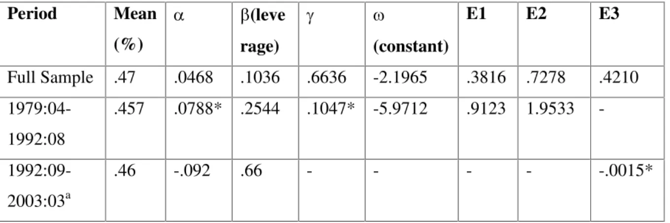
Table VI.2.2. Augmented GARCH19 Model: Conditional Variance with Dummies for Structural Breaks20
Period Mean (%) a b(leve rage) g w (constant) E1 E2 E3 Full Sample .47 .0468 .1036 .6636 -2.1965 .3816 .7278 .4210 1979:04-1992:08 .457 .0788* .2544 .1047* -5.9712 .9123 1.9533 - 1992:09-2003:03a .46 -.092 .66 - - - - -.0015* *not significant a:GARCH(1,1) specification
The results show that the ARCH effects are significantly reduced when large shocks are controlled for. While stock price volatility continues to be persistent series during the full sample period, it is not an explosive series anymore. In fact for pre-liberalization period the ARCH effects completely disappear with the sum of the ARCH coefficients falling to less than .5. A marginal increase in the persistence coefficient is indicated for the post liberalization period but the persistence levels are not high.
All the three dummies have a positive impact on volatility when the full sample is considered. The third dummy has a negative though not significant impact when the second sub period is considered in isolation. No significant economic or political event
19 The model as estimated is EGARCH (1,1) for the full sample and pre liberalization period and
GARCH(1,1) for the post liberalization period. The asymmetric specification is not considered appropriate for the post liberalization period where the returns may belong to a normal distribution.
appears to have occurred at this point in time. The mean level of volatility continues to be unaltered in the two sub periods.
Main conclusions: conventional GARCH model and the augmented model:
Volatility persistence is high for the full sample and sub periods but reduces dramatically when structural changes in the unconditional volatility are factored in the GARCH model.
The period when the economy witnessed the after effects of the BOP crisis and the
initiation of reforms in several fields appears to have been the most volatile period in the stock market between 1979-2003.
Structural shifts in volatility are more likely to be on account of announcement effect
of major economic policy/regime shifts. Incremental changes in policy thereafter do not seem to lead to instability in the market.
Stock market reforms by themselves do not appear to lead to stock return volatility
shifts.
Volatility changes in FII stock buying and selling activity does not coincide with volatility changes in stock return volatility.
Significant developments in the market indicators-turnover or market
capitalization-do not lead to volatility shifts in the stock returns.
There is little evidence of integration of the Indian stock market with the rest of the
world. While the East Asian crisis seems to have affected the stock purchases and sales by FIIs in India, it does not seem to have impacted the stock return volatility.
Domestic financial market and real sector inter-linkages do not appear to have developed as yet in the Indian economy.
Level of volatility does not show much change pre and post liberalization.
Leverage effect is not evident in the monthly data.
The analysis of the time varying pattern of stock market volatility indicates that while it may not be possible to ascribe increase in stock return volatility to FII investment
in the Indian stock market, economic reforms in general, largely announcement and to some extent implementation, lead to an increase in volatility. Incremental change in policy thereafter has only a benign influence on stock return volatility. To analyze this further we undertake an analysis of the stock market cycles in the next section. The bear and bull markets allow us to investigate in greater detail and in an episodic manner, the evolution of stock market instability. Succinctly put, we make an attempt to characterize the evolution of the stock market cycles over time in India and examine if in recent times the stock market cycles have exhibited greater amplitude and volatility. We also examine if the stock market cycles become more volatile specifically around the time of stock market liberalization.
VI.3 Characteristics of Stock Market Cycles
The dynamic impact of financial deregulation on the functioning of capital markets is an aspect that has been considerably less researched. Most studies have focussed on the time - varying volatility of financial markets, which is estimated using ARCH/GARCH models. In contrast there is no analysis of the behavior of stock prices over financial cycles. This lack of analysis is particularly notable in the context of the extensive evidence to establish the link between the momentum based feedback trading by the FIIs, boom-bust stock market cycles and the consequent instability and financial crises21. In this section we examine the possible time varying pattern of stock market cycles in India during 1979-2003. Our focus is on the behavior of “ bear” and “ bull” markets. We construct an anatomy of financial cycles and look at the duration of upturns and downturns in financial markets and the magnitude of the cycles with particular attention to the possibility that the characteristics of the cycles may have changed over time owing to the process of financial liberalization22.
21 The lack of interest in boom-bust cycles is on account of the notion that efficient markets should follow
random walk process. It has however been shown by Cecchetti, Lam and Mark (1990) that even in efficient markets stock prices can follow mean reverting processes. More importantly, however the new theories of asymmetric information in asset markets do support long lasting booms and busts in financial markets.
22 In this section we are not undertaking a pre and post liberalization analysis but only looking at the
The definition of bull and bear markets is as given by Pagan and Soussounov (2003). Bull and Bear phases of stock markets are identified with periods of a generalized upward trend (positive returns) and periods of a generalized downward trend respectively23. Our focus is on duration, amplitude and volatility of the stock market cycles. We attempt to investigate if the stock markets have changed in terms of these characteristics in recent times and more particularly in the aftermath of financial liberalization in India. The period under consideration is one of different regulations regarding international capital mobility, different domestic supervisory systems and exchange rate systems. The diversity of policy and institutional set up therefore allows us to investigate the behavior of bull and bear markets and stock market volatility over time and across economic policy regimes in India.
VI.3.1 Methodology:
The characterization of stock market cycles will allow us to understand the evolution of financial markets. In particular we hope to be able to see if liberalization has magnified the boom-bust cycles in financial markets.
We follow the basic NBER methodology and as a first step identify the cyclical turning points. Essentially, we construct an algorithm so as to isolate the local maxima and minima in a time series, subject to a constraint on the duration of the upturns and downturns. The expansions and contractions are dated for the log level of stock prices.
We adopt a non-parametric approach. The non-parametric approach allows greater flexibility in analysis and allows us to investigate issues related to predictability of the market. The procedure applied looks for periods of generalized upward trend, to be
23 This is a more general definition and emphasizes the expansions and contractions. A definition in terms
of emphasizing extreme movements in the stock prices –i.e. rise (fall) of the market being greater (less) than either 20 or 25% is more appropriate for classification of “ booms” and “ busts” in the market. Our more general definition implies that the stock market has gone from a bull to a bear state if prices have declined for a substantial period since their previous (local) peak. This definition does not rule out
identified as expansions and periods of generalized downward trend to be identified as contractions. The key feature of the analysis is to locate the turning points, peaks and troughs in the series. The turning points define the different phases of the cycle. Pagan and Sossounov (2003) and Gomez Biscarri and Perez de Gracia (2002) first applied the method for stock market analysis. Once the turning points, i.e. the peaks and troughs of the stock index are identified we compute a set of statistics for each phase of the market. We explain below:
Locating the peaks and troughs i.e. points signaling change in the trend of the stock market index:
A peak/trough in the series is defined if pt is highest/lowest in a window of width eight months. We use eight months for a total width of the window of 16 months. There is a peak at t if
[pt-8,…..pt-1<pt>pt+1,……pt+8]
and there is a trough if [pt-8,…..pt-1>pt<pt+1,……pt+8]
To ensure that no spurious phases are identified, the following criteria is used to censor:
Eliminate turns within eight months of the beginning/end of the series
Peaks or troughs next to the end points of the series are eliminated if they are lower/higher than the endpoints
Complete cycles of less than sixteen months of total duration are also eliminated
Phases of less than four months are eliminated unless the fall/rise exceeds 20%24.
After every censoring operation, alternation is enforced so that a peak will always follow a trough and vice versa. Alternation is achieved by taking the highest (lowest) of two consecutive peaks (troughs).
Once the phases are identified we calculate a set of statistics to obtain key information about the behavior of stock prices in each of the phases. The behavior of stock prices is then compared in search for relevant differences over time in stock market evolution. We use a set of measures relating to the shape of the phases of the cycle and to volatility within the cycle. These indicators are defined as follows:
i) Duration (D): Average duration in months of expansions and contractions is calculated as Dbull = 1/NTP
Ê
T t 1 St Dbear = 1/NPTÊ
T t 1 Bt WhereNTP = number of peaks (number of trough to Peak) NPT = number of troughs
And St = total time spent in an expansion
Bt = total time spent in a contraction
ii) Amplitude (A): refers to the total return or total loss from the trough to the peak in a bull market or from the peak to the trough in the case of a bear market.
Abull = 1/NTP
Ê
T t 1 StDpt and Abear = 1/NPTÊ
T t 1 Bt Dptiii) Volatility (V): is measured by the average size of the monthly return in bullish and bear phases: Vbull = 1/
Ê
T t 1 StÊ
T t 1 St|DPt| ; Vbear = 1/Ê
T t 1 BtÊ
T t 1 Bt|DPt|iii) Proportion of big changes: Expansions: B+ = 1/NTP
Ê
T t 1 I[St(1-St+1)Ztbull > .2] Contraction: B- = 1/NTPÊ
T t 1 I[St(1-St+1)Ztbear < .2]Ztbull and Ztbear represent the cumulative return throughout the phase and upto time t. The
indicator function calculates the number phases with amplitude bigger than 0.2 or smaller than -0.2. 25
Results:
The dates of the estimated peaks and troughs are shown in Table VI.3.1 below:
TableVI.3.1: Dates of the Peaks and Troughs
P1 1982:01 T1 1983:04 P2 1986:02 T2 1988:03 P3 1989:07 T3 1990:02 P4 1990:10 T4 1993:07 P5 1994:09 T5 1996:01 P6 1996:06 T6 1996:12 P7 1998:04 T7 1998:10 P8 2000:02 T8 2001:09 P9 2002:03 T9 2002:10
The longest cycles is observed around the time of Gulf crisis and the initiation of economic reforms in India. This cycle is marked by the highest volatility and second largest amplitude among all the cycles observed in the reference period. An informal
25 0.2 is used as a measure of a “ big” phase given that a 20% return/loss is the rule of thumb traditionally
analysis shows that external linkages seem non existent prior to 1998. T7 onwards, i.e. after October 1998, coincidence even with US markets is visible. Specifically for the 2000 peak (P8) a coincidence of peaks all across the US and the emerging markets is seen26.
Table VI.3.2: Characteristics of the Bull and Bear Markets Bull
Full Sample Pre Post
D 15.7 21 11.4
A .58 .77 .44
V .813 1.03 .64
B+ 8/9 4/4 4/5
Bear
Full Sample Pre Post
D 14.9 15.7 14.5
A -.23 -.22 -.24
V .546 .62 .51
B- 6/9 1/3 5/6
In general, the bull phases are longer, the amplitude of bull phases is higher and the volatility in bull phases is also higher. By itself though the bull phase in comparison with its pre liberalization character is more stable.
Duration: The mean duration of contractions (bear markets) is around 15 months and that for expansions (bull markets) is 16 months for the full sample period. The average duration of contractions falls from around 16 months in the pre liberalization period to 14.5 in the post liberalization period. In case of expansions the fall in average duration is more apparent. While in the pre liberalization period the average duration of the expansion is 21 months this has fallen to around 11 months in the post liberalization period. The cycles have therefore dampened in the recent past.
Amplitude27: The expansions are more volatile and more so in the pre liberalization period. The average gain during expansions is 58% for the full sample and 77% for the pre liberalization period probably as a compensation for the excessive volatility. The amplitude falls to 44% in the post liberalization period as also the volatility in the bull phase. The same is however not true of the contractions which have become marginally more volatile in the post liberalization period. The post lib amplitude of contractions at 24% is higher than the 23 and 22 % in the full sample and pre liberalization period respectively. The gains during expansions are larger than the losses during the bear phases of the stock market cycles.
Volatility: Volatility of the bull phases is far greater than the bear phases. Volatility declines in the post liberalization phase for both the bull and bear phase with the decline being greater for the former phase of the cycle. In both the bull and the bear phases however volatility is greater for the pre liberalization period than either the post or the full sample period.
Big expansions and Contractions: Bear phases have been bigger in the post reform phases than in the pre reform sub-sample. As shown by our results all except one contractions in the post reform period have been large.
Our analysis shows that financial cycles have not intensified after financial liberalization. Financial liberalization does tend to trigger more explosive financial cycles in the short run. A generalized reduction in instability in the post reform period is thus observed28.
VII Conclusions
In this paper we have examined the time varying pattern of stock return volatility in India over the period 1979-2003 using monthly stock returns and asymmetric GARCH
27 Measures the percentage change in the equity price over a phase.
28 Interestingly these findings are in line with the nature of evolution of financial cycles in the other
methodology. We have also examined sudden shifts in volatility and the possibility of coincidence of these sudden shifts with significant economic and political events both of domestic and global origin. Stock market cycles have also been analyzed for variation in amplitude, duration and volatility of the bull and bear phases over the reference period.
Our analysis reveals that liberalization of the stock market or the FII entry in particular does not have any direct implications for the stock return volatility. No structural changes in the stock price volatility around any liberalization event or more importantly around the dates of breaks for volatility in FII sales and purchases in India are observed. The apparent link generally drawn between stock price volatility and the sudden withdrawal or heavy purchases by the FIIs i.e. the volatile FII investment in the stock market does not seem to hold true for India. Reforms in general lead to a structural shift in the volatility in India. In all the phases as delineated by our structural break analysis, the period between 1991:05 and 1993:12 is the most volatile period with the standard deviation of stock returns exceeding that in the other periods.
The analysis of the stock market cycles shows that in general over the reference period the bull phases are longer, the amplitude of bull phases is higher and the volatility in bull phases is also higher. The gains during expansions are larger than the losses during the bear phases of the stock market cycles. The bull phase in comparison with its pre liberalization character is more stable in the post liberalization phase. The results of our analysis also show that the stock market cycles have dampened in the recent past. Volatility has declined in the post liberalization phase for both the bull and bear phase of the stock market cycle.
APPENDIX
I. All Break Dates:
Variable No. of change points* Dates Event VSensex 3 1983:02 1984:12 P: IG assassination (31.10.1984)
1986:09 E: Launch of country fund –India Country Fund
1990:05 1993:12
1998:01 E: Downgrading of India’s Credit Rating
VIFCG 3 1990:02 1992:01 1994:11 1997:02 1999:01 VFII(P) 2 1995:02 1996:03 1996:05 1997:09 E: EA crisis 1999:11 2001:02 VFII(S) 2 1995:02 1996:05 1996:11 1997:08 E: EA crisis 1999:11 2001:02
*Number of significant changes. Significant dates are in bold. P:Political Event, E:Economic Event
II. 1990:05 -1993:11: Main Financial and Political Events
Date Event
1990
01-05 Liberalization of foreign investment policy
1991
24-07 Liberalization of regulations on FDI
09-10 Rationalization of interest rates
91-92 SEBI made the regulatory agency for the capital market of India
1992
Introduction of insider trading laws Introduction of CRAR
00-02 First ADR announced
01-03 Dual exchange rate system was created
00-05 First international equity offering by RIL
29-05 Abolition of CCI
00-06 First exchange traded overseas listing
01-06 ADR effective date – RIL
00-09 FII policy announcement
00-11 Entry of FIIs
1993
Entry restrictions for banks eased
00-03 Series of bombing in Bombay
01-03 Rupee was made fully convertible
07-93 Essar Gujrat launched India’s first Euro-convertible bond
17-08 Enactment of “ Recovery of Debts due to Banks and Financial Institutions Act, 1993”
References
Aggarwal, R., C.Inclan and R. Leal (1999) “ Volatility in Emerging Stock Markets” ,
Journal of Financial and Quantitative Analysis 34.
Andreou Elena and Eric Ghysels (2002) “ Detecting Multiple Breaks in Financial Market
volatility Dynamics” Discussion Paper 2002-02, Department of
Economics, University of Cyprus
Bai, Jushan and Pierre Perron (1998) “ Estimating and Testing Linear Models with Multiple Structural Changes” Econometrica, Vol.66(1), 47-78.
Bai, Jushan and Pierre Perron (2003) “ Critical Values for Multiple Structural change Tests” .
Bekaert, Geert and Campbell R. Harvey. (2000) “ Foreign Speculators and Emerging Equity Markets” , The Journal of Finance, 55 (2) April.
Bekaert, G., Harvey, C.R. and R.L. Lumsdaine (2002) “ The Dynamics of Emerging
Market Equity Flows” , Journal of International Money and Finance 21
Bekaert, G., Harvey, C.R. and R.L. Lumsdaine (2002) “ Dating the Integration of World Capital Markets” , Journal of Financial Economics 65.
Bekaert, G., Harvey, C.R. and A. Ng (2002) “ Market Integration and Contagion” , mimeo. Biscarri, Javier Gómez and Fernando Pérez de Gracia (2003) “ Stock Market Cycles and Stock Market Development in Spain” Facultad de Ciencias Económicas y
Empresariales Working Paper.
Black, Fischer, (1976) “ Studies of Stock Price Volatilty changes” Proceedings of the American Statistical Association Annual Meetings.
Cecchetti, S. P.Lam and N. Mark (1990) “ Mean Reversion in Equilibrium Asset Prices” ,
American Economic Review 80(3)
De Santis, Giorgio and S. Imrohoroglu (1997) “ Stock Returns and Volatility in Emerging
Financial Markets” , Journal of International Money and Finance 16
(August) 561-579.
Edwards, Sebastian, Javier Gómez Biscarri, Fernando Pérez de Gracia (2003). “ Instability, Financial Liberalization and Stock Market Cycles”
Edwards, Sebastian, Javier Gómez Biscarri, Fernando Pérez de Gracia (2003).“ Stock Market Cycles, Financial Liberalization and Volatility” National Bureau for Economic Research Working Paper No. 9817.
Edwards, Sebastian and Raul Susmel (2000). “ Interest Rate Volatility and Contagion in
Emerging Markets: Evidence from the 1990s” National Bureau for
Economic Research Working Paper No. 7813.
Engle, Robert and C. Mustafa (1992) “ Implied ARCH Models from Options Prices”
Journal of Econometrics 52.
Folkerts-Landau, D., and T. Ito. 1995. International Capital markets: Developments, Prospects and Policy Issues, International Monetary Fund.
Forbes, K. and R. Rigobon (2002) “ No Contagion, only Interdependence: Measuring
Stock Market Comovements” Journal of Finance 57.
Hamilton J.D. and R. Susmel (1994) “ Autoregressive Conditional Heteroscedasticity and
Changes in Regime” Journal of Econometrics, 64.
Inclan, Carla and George C. Tiao (1994) “ Use of Cumulative Sums of Squares for
Retrospective Detection of Changes of Variance” Journal of the American
Statistical Association, 89 (427)
Kaminsky Graciela Laura and Sergio L. Schmukler (2002). “ Short-Run Pain, Long-Run Gain: The Effects of Financial Liberalization”
Kaminsky, Graciela, L and Carmen M. Reinhart (2001). “ Financial Markets in Time of Stress” .
Kaminsky, Graciela Laura and Sergio L. Schmukler (2001). “ On Booms and Crashes: Financial Liberalization and Stock Market Cycles” .
Kaminsky, Graciela and Sergio Schmuckler (1999) “ On Booms and Crashes: Stock Market Cycles and Financial Liberalization” .
Kim, E.H. and V. Singal (1997) “ Opening up of Stock Markets: Lessons from Emerging Economies” Virginia Tech. Working Paper.
Kwan, B.F. and M.G. Reyes (1997), “ Price Effects of Stock market Liberalization in
Taiwan” , The Quarterly Review of Economics and Finance 37.
Lamoureux, Christopher G. and William D. Lastrapes (1990) “ Persistence in Variance,
Structural Change and the GARCH Model” , Journal of Business and
Economic Statistics, Vol.8(2)
Lastrapes, W.D. (1989) “ Exchange Rate Volatility and US Monetary Policy: An ARCH Application” Journal of Money, Credit and Banking, 21.
Lanne, Markku and Pentti Saikkonen. “ Nonlinear GARCH Models for Highly Persistent Volatility” mimeo.
Levine, Ross and Sara J. Zervos. (1995) “ Capital Control Liberalization and Stock Market Performance” .( Unpublished; Washington: World Bank)
Maekawa, Koichi, Sangyeol Lee, and Yasuyoshi Tokutso “ A Note on Volatility Persistence and Structural Changes in GARCH Models” , mimeo.
Maekawa, Koichi, Sangyeol Lee, and Yasuyoshi Tokutso. “ Structural Change and Spurious Volatility Persistence” mimeo.
Nilsson, Birger. (2002) “ Financial Liberalization and the Changing Characteristics of Nordic Stock Returns” , Department of Economics Lund University.
Pagian, Adrian, R and Kirill A. Sossounav (2003) “ A Simple Framework for Analyzing Bull and Bear Markets” Journal of Applied Econometrics 18
Rigobon, R., (2003) “ On the Measurement of International Propagation of Shocks:Is it Stable?” Journal of International Economics.
Shenbagaraman, Premalata, “ Do Futures and Options Trading Increase Stock Market Volatility” , mimeo.
Shiller, R.J. 1989 Market Volatility MIT Press, Cambridge, MA.
Tauchen, George E. and Mark Pitts (1983), “ The Price Variability – Volume Relationship on Speculative Markets” , Econometrica 51(2)
Wang ,Shiyun “ High Frequency Returns Mean Reversion and Volatility Persistence” , University of Manchester.
Yardeni, Edward Dr., Amalia F. Quintana and Joseph Abbott (2002) “ Stock Market Cycles” Prudential Financial Research.