Output dynamics in an endogenous growth model
Ilaski Barañano M. Paz Moral
Departamento de Fundamentos del Análisis Económico I. Universidad del País Vasco
Departamento de Economía Aplicada III. Universidad del País Vasco
Abstract
The aim of this paper is to assess the importance of RBC models with endogenous growth in characterizing the observed output dynamics. In particular, this article considers a stochastic version of Lucas' (1988) model in the absence of externalities in discrete time with two modifications: agents do not only derive utility from consumption but also from leisure and labor adjustment costs are included. Results reveal that combining the endogenous character of the engine of growth with labor adjustment costs may help solve the Cogley−Nason (1995) puzzle since, it provides a stronger propagation mechanism and this, in the end, improves the model's ability to generate realistic output dynamics.
Citation: Barañano, Ilaski and M. Paz Moral, (2003) "Output dynamics in an endogenous growth model." Economics Bulletin, Vol. 5, No. 15 pp. 1−13
Submitted: July 1, 2003. Accepted: October 6, 2003.
1. Introduction
As Cogley and Nason (1995) noted, standard Real Business Cycle (RBC) models fail to reproduce two stylized facts about U.S. output dynamics: first, GNP growth is positively autocorrelated over short horizons and has a weak and possibly insignificant negative autocorrelation over longer horizons; and second, GNP appears to have an important trend-reverting component that has a hump-shaped MA representation. Fur-thermore, these authors find that standard RBC models have weak internal propagation mechanisms and, as a consequence, they need exogenous sources of dynamics in order to replicate observed autocorrelation and impulse response functions. Non-standard RBC models that incorporate lags or costs of adjusting labor input are only partially suc-cessful, since they also need implausibly large transitory shocks in order to match the transitory impulse response function found in data. As a result, they suggest that “RCB theorists ought to devote further attention to modeling internal sources of propagation”. The traditional approach in RBC literature has been to assume a strict exogenous engine of growth and, as is well known, many models do need a second source of uncer-tainty in order to conform the fluctuations observed in U.S. labor market. An alternative approach is to consider a model that encompasses both cycles and endogenous growth. This paper pursues this second line of research.
Many authors have already incorporated endogenous sources of growth in RBC mo-dels and shown that this line of research can lead to substantial improvements upon their exogenous growth relatives. Gomme (1993), Ozlu (1996), Einarsson and Marquis (1997) and Bara˜nano (2001), among others, have shown that endogenous growth mo-dels not only perform better than the standard exogenous growth model in explaining labor market fluctuations but also provide a stronger propagation mechanism1
. Her-cowitz and Sampson (1991), Perli and Sakellaris (1998), Jones, Manuelli and Siu (2000) and Matheron (2003) have also analyzed the cyclical properties of endogenous growth models. They incorporate endogenous sources of growth in dynamic stochastic general equilibrium models and show that doing so permits, among other things, to display the kind of internal propagation mechanisms that are necessary to match the observed autocorrelation of output growth. However, they do not study their models’ ability to reproduce the trend reverting component found in U.S. GNP. This paper is closely linked to that of Collard (1999). He also assesses the ability of endogenous growth models in solving the Cogley-Nason (1995) puzzle, but due to the specific set of functional forms used (he considers log-linear specifications for preferences and technology which allow him to obtain an analytic solution of output growth), his model fails in one aspect, since it predicts that output, consumption and investment are perfectly correlated, which is obviously counterfactual.
1
Endogenous growth models have also been used to explain economic growth in the long-run. Lucas (1988), Rebelo (1991) and King and Rebelo (1990), among others, focus on the ability of endogenous growth models to explain certain observed growth patterns which the standard exogenous growth model fails to account for. Furthermore, as noted by King and Rebelo (1993), the transitional dynamics of the basic exogenous growth model in order to explain sustained cross-country differences in growth rates
The aim of this paper is to assess the importance of RBC models with endogenous growth in characterizing the observed output dynamics without constraining the specific set of functional forms used to obtain a closed-form solution. In particular, this article considers a stochastic discrete time version of Lucas’ (1988) human capital accumulation model with two modifications: agents do not only derive utility from consumption but also from leisure and labor adjustment costs are included2
. Results reveal that com-bining the endogenous character of the engine of growth with labor adjustment costs may help solvethe Cogley-Nason (1995) puzzle since, it provides a stronger propagation mechanism and this, in the end, improves the model’s ability to reproduce the above mentioned observations.
The rest of the paper is as follows: Section 2 describes the endogenous growth model considered and the calibration procedure used. In Section 3, the quantitative results obtained are shown. Finally, Section 4 concludes.
2. The Model
This paper considers a stochastic discrete time version of Lucas’ (1988) model in the absence of externalities with two modifications. On the one hand, agents do not only derive utility from consumption but also from leisure. On the other hand, as suggested by Shapiro (1986) and Cogley and Nason (1995), labor adjustment costs are included.
The economy consists of a large number of productive families which own both the production factors and the technology used in two production activities: the production of the final good (market sector) and the production of new human capital (human ca-pital sector)3
. The population size is assumed to be constant. At any point in time, individuals must decide what fraction of their time they devote to each of these activi-ties, and how much time they set aside for leisure. The time endowment is standardized to one, so thatlt denotes the fraction of time given over to leisure andnt the fraction of time devoted to the production of the consumption good.
The technology of the consumption good is described by a production function with constant returns to scale with respect to physical capital and efficient labor. As suggested by Shapiro (1986) and Cogley and Nason (1995), we also consider quadratic adjustment costs in labor input. This specification implies that the marginal cost of adjusting the labor input increases in the rate of employment. Formally, the production technology is made (log) linear in the cost of adjustment,
ln yt = ln[AmZtktα(ntht)1−α ]− η 2 ∆(ntht) nt−1ht−1 2 , with 0< α <1 (1) where ntht represents the qualified labor units, Am is the parameter which measures the productivity of this sector, kt and ht are the stocks of physical capital and human
2
Co-movements of other variables with output and the relative volatilities of various series for this endogenous growth model without labor adjustment costs are studied in Bara˜nano (2001).
3
The introduction of a home production sector competing with the market sector has already been used in RBC literature. See for example Benhabibet al. (1991), Greenwood and Hercowitz (1991),
capital in per-capita terms, respectively,η is the labor adjustment cost parameter, and finally Zt is a technology shock characterized by the following autoregressive process:
ln(Zt) =ρ2 ln(Zt−1) + (1−ρ2) ln( ¯Z) +εt, εt ∼iid(0, σZ). (2) The law of motion for physical capital is
kt+1 =yt−ct+ (1−δk)kt, (3)
wherectis consumption andδkrepresents the depreciation rate of physical capital, which is assumed to be constant.
New human capital is assumed to evolve according to the following equation:
ht+1 =Ahθt(1−lt−nt)ht+ (1−δh)ht, (4) where Ah measures the productivity of this sector, δh denotes the depreciation rate of human capital andθt is a shock which follows an AR(1) process given by:
ln(θt) =ρ1 ln(θt−1) + (1−ρ1) ln(¯θ) +t, t∼iid(0, σθ). (5) It is assumed that consumers derive their utility from the consumption of the final good and from leisure. Future utility is discounted at a rateβ.
As is well known, in the absence of external effects, public goods and distortionary taxation, the solution to the planner’s problem is the competitive equilibrium allocation. The problem faced by the central planner is to choose sequences for consumption, hours worked, leisure, physical capital and human capital devoted to the market sector that maximize the discounted stream of utility given by4
: max nt,ct,lt,kt+1,ht+1 E0 ∞ X t=0 βt[λlnct+ (1−λ) lnlt], 0≤λ≤1,
subject to (1),(2),(3),(4),(5), the usual non negativity constraints, 0 ≤ lt ≤ 1,0 ≤ 1−lt−nt ≤1 and given an initial condition (Z0, θ0,k0, h0,n0).
2.1 Calibration
In order to solve and simulate the model, we must assign values to the parameters. The calibration procedure followed is that suggested by Kydland and Prescott (1982). The values for structural parameters and some steady state variables are displayed in Table I and, except for η, they are explained in detail in Bara˜nano (2001). The labor adjustment parameter, η, has been calibrated from estimates in Shapiro (1986). Fol-lowing Cogley and Nason (1995) we take η = 0.36 as the baseline value and we check whether the results are sensitive to changes inη. These authors point out that this value
4
Note that this function satisfies the conditions needed to ensure the existence of a balanced growth path. For more details on this issue, see King, Plosser and Rebelo (1988, pp. 201-202).
probably overstates the size of aggregate labor adjustment costs. However, when human capital is included, labor is measured in efficiency units and, as a consequence, not only the hours worked but also human capital are subject to adjustment costs. Hence, the same baseline value seems to be more suitable when human capital is included than in an exogenous growth model.
3. Results
The purpose of this paper is to analyze whether endogenous growth RBC models are consistent with two stylized facts about output dynamics in the U.S. documented by an extensive empirical literature on the time series properties of aggregate output5
. First, GNP growth is positively correlated over short horizons and has weak and possi-bly insignificant negative autocorrelation over long horizons. Second, GNP appears to have an important trend-reverting component that has a hump-shaped impulse response function. The procedure can be summarized as follows. We generate artificial time series for output by simulating various RBC models. The resolution method used in this paper is Uhlig’s (1999) Log-Linear Method6
. Autocorrelation and impulse response functions were estimated for each artificial sample (each model was simulated 1000 times) and then we compared our results with U.S. data from 1955:3 to 1984:1. Results were collected into empirical probability distributions used to calculate the probability of observing the statistics estimated from U.S. data under the hypothesis that the data were generated by a particular RBC model. Formally, this procedure can be regarded as a specification test of a particular RBC model that can also be used as an informal guide to model reformulation.
Four RBC models are considered: a standard exogenous growth model without labor adjustment costs, a standard exogenous growth model with labor adjustment costs, Lucas’ (1988) model without labor adjustment costs and Lucas’ (1988) model with labor adjustment costs.
A. Autocorrelation Functions
We analyze whether the above mentioned models replicate the sample autocorrelation function (ACF) for output growth. We follow Cogley and Nason (1995) and compute generalized statistics to test the match between sample and theoretical ACF’s:
Qacf = (bc−c)0b
Vc−1(bc−c),
where bc is the sample ACF and c is the model generated one, which was estimated by averaging the ACF’s of 1000 samples simulated by the model. Matrix Vcb denotes the covariance matrix of these simulated ACF’s. GeneralizedQstatistics are approximately
χ2
(p), wherepis the number of lags inc. Following Cogley and Nason (1995), we report the results forp= 8.
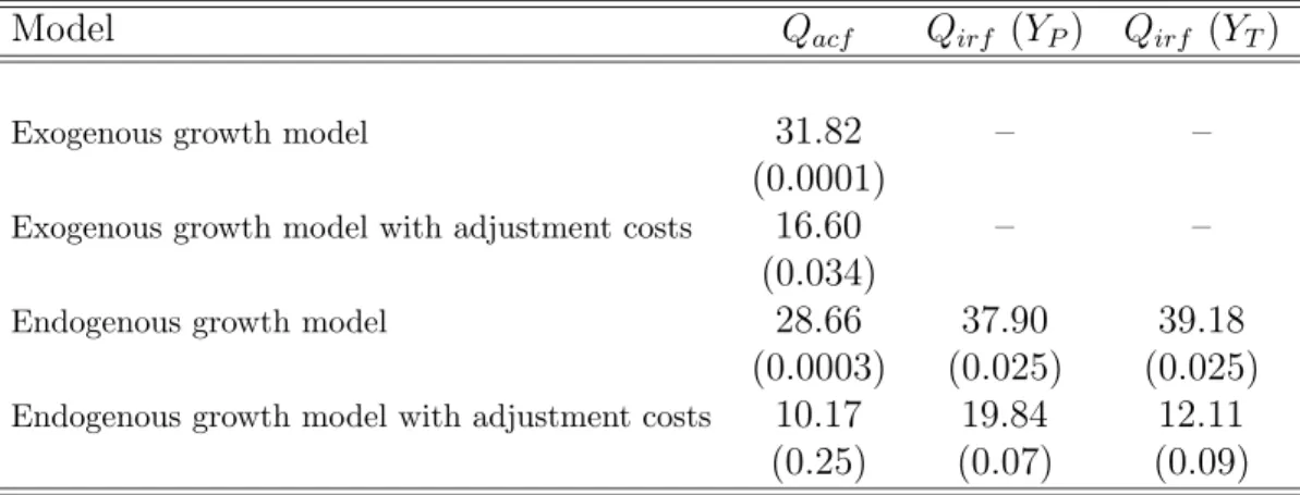
The first column of Table II reportsQacf statistics for each model. Probability values are in parentheses. Results show that the adjustment cost endogenous growth model is the only one that passes the autocorrelation test, but this result is not robust to changes in the value of η since the model is rejected when η = 0.36
4 at 5% significance level but 5
See, for example, Nelson and Plosser (1982), Watson (1986), Campbell and Mankiw (1987), Cochrane (1988) and Blanchard and Quah (1989).
6
it is not rejected at 2.5% (see the first column of Table III).
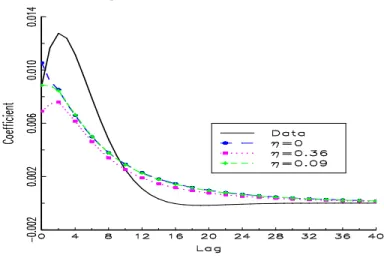
Figure 1 illustrates the results for each model. The solid line show the sample ACF and dotted lines show artificial ACF’s. Note that labor adjustment costs are crucial for generating serial correlation in both exogenous and endogenous growth models. These results are sensitive to changes in the value of η. Once this specification is considered, the endogeneity of the technological progress improves the model’s ability to replicate the observed ACF. The propagation mechanism embodied in the model provides some intuition for these results.
B. Impulse Response Functions
We also analyze whether those models replicate observed impulse response functions (IRF’s). The IRF’s are obtained by using the structural VAR technique developed by Blanchard and Quah (1989). For the implementation of this technique, a second-order VAR was estimated for per-capita output growth and hours worked. We follow Cogley and Nason (1995) and compute the following statistic to test the match between sample and theoretical IRF’s :
Qirf = (rb−r)0b
Vr−1(br−r),
where br is the sample IRF and r is the model-generated one, which was estimated by averaging the IRF’s of 1000 samples simulated by the model. Matrix Vbr denotes
covari-ance matrix of this simulated IRF’s. Following Cogley and Nason (1995), we truncate again at lag 8.
The second and third columns of Table II reportQirf statistics for each model. Monte Carlo probability values are in parentheses. (Exogenous growth models are driven by a single shock, so their bivariate VAR’s have stochastic singularities). We infer from this table that results improve when the adjustment cost endogenous growth model is considered. This model has some success at matching not only the permanent IRF but also the transitory IRF. In the former dimension, results are sensitive to changes in the value ofη, but, in the latter dimension, the model passes the test even when η= 0.36
4 at the 5-percent level.
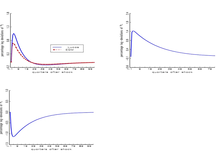
Figure 2 illustrates the IRF’s for Lucas’ (1988) model. The solid lines show the sam-ple IRF’s and the dotted lines show artificial IRF’s. The adjustment cost endogenous growth model generates a hump in the transitory IRF as shown in the data. Results are sensitive to the choice ofη. As shown in Figure 2, the higher the labor adjustment cost parameter, the higher the hump displayed.
Hence, it follows from the results that incorporating labor adjustment costs into the model improves its ability to reproduce the observed ACF, but an endogenous propaga-tion mechanism is also needed in order to obtain realistic output dynamics.
C. Propagation Mechanism
Cogley and Nason (1995) argue that standard RBC models cannot generate the right pattern of output dynamics via their internal structure due to the weakness of the prop-agation mechanism embodied in them. Indeed, they must rely on external sources of dynamics to replicate both stylized facts7
. In this section we analyze the internal prop-agation mechanism of the four models considered.
In order to asses the importance of the propagation mechanism embodied in these four models, we analyze the dynamic response functions of hours and output to shocks in Zt and θt. Note that, although the specification considered for both models is an AR(1) process, the former can be interpreted as a transitory shock and the latter as a permanent shock, since technology shocks, unlike human capital shocks, do not affect the growth rate.
In comparison with the standard exogenous growth model (EGM), Lucas’ (1988) model provides a stronger internal propagation mechanism due to the fact that indi-viduals not only substitute between market activity at different dates but also between market and human capital accumulation activities at a point in time. In particular, they respond to favorable technology shocks by devoting more time to work, while in periods of recession they respond by accumulating more human capital, maintaining a smooth path for leisure. Figure 3 reports the response of hours and output to a 1% technology shock in both models. This figure shows that hours fluctuate much more when this second sector is considered8
.
The ACF for output growth depends on the effects caused by both transitory and permanent shocks. In response to a favorable transitory shock, labor flows into the mar-ket and out of the human capital sector, causing output to increase at impact. Due to the presence of labor adjustment costs, firms do not adjust labor input completely in the current quarter. Their optimal response is to defer a part to the subsequent quarter. Hence, output rises again in the subsequent period. Eventually, the income effect of a technology shock begins to offset the substitution effect, causing hours and output to decline from their peak. This generates a hump-shaped IRF of output to technology shocks (see transitory IRF in figure 2). Thus, a favorable technology shock generates positive autocorrelation in the transitory component of output growth. As shown in figure 3, not only the impact effect of a technology shock but also the lagged effects are larger than in the EGM. This generates a stronger serial correlation in output growth.
Apart from this effect we must take into account that which is caused by a perma-nent shock. Figure 3 also reports that, when a favorable permaperma-nent shock takes place, output falls at impact and is followed by further small declines. Subsequently, as human capital productivity declines, output rises back toward its initial trend. Thus, a positive
7
They find that standard exogenous growth models strongly damp transitory shocks, so most of the variation in output growth is due to permanent movements, which means that output dynamics are nearly the same as impulse dynamics.
8
By internal propagation mechanism we mean those forces or properties of the model that amplify the effect of the technology shock and cause the deviation from the steady state to persist. As Bara˜nano (2001) pointed out, when a single shock is considered, Lucas’ (1988) model needs a lower technology shock in order to reproduce the volatility of U.S. output. We also infer from this result that Lucas’(1988) model provides a stronger propagation mechanism.
human capital shock also generates positive autocorrelation in the permanent compo-nent of output growth. Hence, this second effect generates a stronger serial correlation in output growth. Notice that this second effect only takes place when this second sector is included.
To sum up, the introduction of labor adjustment costs in Lucas’ (1988) endogenous growth model allows for some improvements in explaining two stylized facts about output dynamics in the U.S.: a positive autocorrelation of output growth and an important trend reverting component in GNP that has a hump-shaped transitory impulse response function. But it must be noticed that autocorrelation results depend on the size of the labor adjustment costs considered. We infer from this result that, as suggested by Cogley and Nason (1995), RBC theorists should devote further attention to the internal propagation mechanisms embodied in RBC models.
4. Conclusions
As Cogley and Nason (1995) noted, standard RBC models fail to reproduce two stylized facts about U.S. output dynamics: GNP growth is positively autocorrelated in the short run and has a weak negative autocorrelation over longer horizons, and GNP appears to have an important trend-reverting component that has a hump-shaped IRF. Furthermore, these authors find that standard RBC models must rely on external sources of dynamics to replicate both stylized facts due to the weakness of their internal prop-agation mechanisms. Non-standard RBC models that rely on lags or costs of adjusting labor input are only partially successful, since they also need implausibly large transitory shocks in order to match the transitory IRF found in data. As a result, they suggest that RCB theorists ought to devote further attention to understanding how shocks are magnified and propagated over time.
The aim of this paper is to assess the importance of RBC models with endogenous growth in characterizing the observed output dynamics without constraining the specific set of functional forms used to obtain a closed-form solution. In particular, this article considers a stochastic version of Lucas’ (1988) model in the absence of externalities in discrete time with two modifications: agents do not only derive utility from consump-tion but also from leisure, and labor adjustment costs are included. Results reveal that combining the endogenous character of the engine of growth with labor adjustment costs may help solvethe Cogley-Nason (1995) puzzle, since it provides a stronger propagation mechanism and this, in the end, improves the model’s ability to reproduce the above mentioned observations.
Figure 1: ACF for output growth
Figure 2: Impulse-response function from the Blanchard-Quah technique
Figure 3: Response function
Table I. Parameter and steady state valuesa.
Parameters Value Interpretation
β 0.9936 Subjective discount factor
α 0.36 Share of physical capital in the final good technology
δk 0.025 Depreciation rate of physical capital
δh 0.005 Depreciation rate of human capital
Am 1 Scale parameter in the final good technology
Ah 0.0266666 Scale parameter in the human capital production function
λ 0.3769 Consumption weight in utility
η 0.36 Size of labor adjustment costs
σZ 0.007 Standard deviation ofεt σθ 0.004 Standard deviation oft ρ1 0.95 Persistence ofθt ρ2 0.95 Persistence ofZt v 0.0036 Growth rate ¯ n 0.24 Hours worked a
For parameters with a time dimension, the unit of time is a quarter of a year.
Table II. Test statistics for the autocorrelation and impulse response func-tions
Model Qacf Qirf (YP) Qirf (YT)
Exogenous growth model 31.82 – –
(0.0001)
Exogenous growth model with adjustment costs 16.60 – –
(0.034)
Endogenous growth model 28.66 37.90 39.18
(0.0003) (0.025) (0.025)
Endogenous growth model with adjustment costs 10.17 19.84 12.11
(0.25) (0.07) (0.09)
Table III. Sensitivity analysis
Endogenous growth model with adjustment costs Qacf Qirf (YP) Qirf (YT)
η= 0.36 10.17 19.84 12.11 (0.25) (0.07) (0.09) η= 0.36 2 12.54 22.79 16.58 (0.128) (0.058) (0.064) η= 0.36 4 16.03 27.22 22.85 (0.041) (0.042) (0.051)
References
Bara˜nano, I. (2001) “On human capital externalities and aggregate fluctuations” Jour-nal of Business and Economics 53, 459-472.
Benhabib, J., Rogerson R., and R. Wright (1991) “Homework in macroeconomics: Household production and aggregate fluctuations” Journal of Political Economy 99, 1166-87.
Blanchard, O. J., and D. Quah (1989) “The Dynamic Effects of Aggregate Demand and Supply Shocks” American Economic Review 79, 655-673.
Campbell, J. Y., and N. G. Mankiw (1987) “Are Output Fluctuations Transitory?”
Quarterly Journal of Economics 102, 857-80.
Cochrane, J. H. (1988) “How Big Is the Random Walk in GNP?” Journal of Politi-cal Economy 96, 893-920.
Cogley, T., and J. M. Nason (1995) “Output Dynamics in Real-Business-Cycle Mo-dels” American Economic Review 85, 492-511.
Collard, F. (1999) “Spectral and persistence of cyclical growth” Journal of Economic Dynamics and Control 23, 463-488.
Einarsson, T., and M. H. Marquis (1997) “Home production with endogenous growth”
Journal of Monetary Economics 39, 551-569.
Gomme, P. (1993) “Money and Growth revisited: Measuring the costs of inflation in an endogenous growth model”Journal of Monetary Economics 32, 51-77.
Greenwood, J., and Z. Hercowitz (1991) “The allocation of capital and time over the business cycle”Journal of Political Economy 99, 1188-1214.
Jones, L., Manuelli, R., and H. Siu (2000) “Growth and Business Cycles” NBER working paper 7633.
Hercowitz, Z., and M. Sampson (1991) “Output growth, the real wage, and employ-ment fluctuations”American Economic Review 81, 1215-1237.
King, R., Plosser C., and J. Rebelo (1988) “Production, Growth and Business Cycles: I. The basic Neoclassical Model” Journal of Monetary Economics 21, 195-232(a).
King, R., and J. Rebelo (1993) “Transitional Dynamics and Economic Growth in the Neoclassical Model” American Economic Review 83, 908-31.
King, R., and J. Rebelo (1990) “Public Policy and Economic Growth: Developing Neo-classical Implications” Journal of Political Economy 98, 126-150.
Econometrica 50, 1345-70.
Lucas, R. E., Jr. (1988) “On the mechanics of economic development”Journal of Mon-etary Economics 22, 3-42.
Matheron, J. (2003) “Is growth useful in RBC models?” Economic Modelling 20, 605-622.
Nelson, C. R., and C. I. Plosser (1982) “Trends and Random Walks in Macroeconomic Time Series”Journal of Monetary Economics 10, 139-62.
Ozlu, E. (1996) “Aggregate Economic Fluctuations in Endogenous Growth Models”
Journal of Macroeconomics 18, 27-47.
Perli, R., and P. Sakellaris (1998) “Human capital formation and business cycles persis-tence”Journal of Monetary Economics 42, 67-92.
Rebelo, S. (1991) “Long-Run Policy Analysis and Long-Run Growth” Journal of Polit-ical Economy 99, 500-521.
Shapiro, M. D. (1986) “The Dynamic Demand for Capital and Labor”Quarterly Journal of Economics 101, 513-542.
Uhlig, H. (1999) “A toolkit for analyzing nonlinear dynamic stochastic models easily” inComputational Methods for the Study of Dynamic Economics by Marimon, R., Scott, A., Eds., Oxford University Press, Oxford.
Watson, M. W. (1986) “Univariate Detrending Methods with Stochastic Trends”Journal of Monetary Economics 18, 49-76.