Copula-based semiparametric models for multivariate time series

Contents lists available atSciVerse ScienceDirect

Journal of Multivariate Analysis

journal homepage:www.elsevier.com/locate/jmva

Copula-based semiparametric models for multivariate time series

Bruno Rémillard

∗

, Nicolas Papageorgiou, Frédéric Soustra

HEC Montréal and BNP Paribas, NY, United States

a r t i c l e i n f o

Article history:

Available online 23 March 2012

AMS subject classifications:

primary 62H12 62H15 secondary 60G10 60J05 Keywords: Conditional copulas Markov models Pseudo likelihood Ranks

a b s t r a c t

The authors extend to multivariate contexts the copula-based univariate time series modeling approach of Chen & Fan [X. Chen, Y. Fan, Estimation of copula-based semiparametric time series models, J. Econometrics 130 (2006) 307–335; X. Chen, Y. Fan, Estimation and model selection of semiparametric copula-based multivariate dynamic models under copula misspecification, J. Econometrics 135 (2006) 125–154]. In so doing, they tackle simultaneously serial dependence and interdependence between time series. Their technique differs from the usual approach to time series copula modeling in which the series are first modeled individually and copulas are used to model the dependence between their innovations. The authors discuss parameter estimation and goodness-of-fit testing for their model, with emphasis on meta-elliptical and Archimedean copulas. The method is illustrated with data on the Canadian/US exchange rate and the value of oil futures over a ten-year period.

©2012 Elsevier Inc. All rights reserved. 1. Introduction

Proper understanding and modeling of the dependence between financial assets is an important issue. The 2008 financial crisis provided us with a very concrete example of the devastating financial and economic consequences of overly naive and simplistic assumptions about default contagion.

In order to help prevent future financial crises, robust methods must be developed to model dependence between multiple time series. At present, most of the work dealing with the issue relies on Pearson’s correlation as a measure of dependence; see [11] for a review. Unless the series are jointly Gaussian, however, correlation can be a poor measure of dependence [13]. Copulas are a much more flexible tool for dependence modeling.

As explained by Patton in this Special Issue [34], there are typically two ways to exploit copulas in time series modeling. Copulas can be used either to model the dependence between successive values of a univariate time series, or to model the conditional dependence of a random vector, given some information about its past, thereby leading to time-varying copulas. See [33] for an earlier review of copula modeling of financial time series.

In most papers advocating copula-based models for multivariate time series, serial dependence is either ignored or treated separately from interdependence. When serial dependence is taken into account, the individual series are typically modeled first, and a copula is used to capture the dependence between serially independent innovations; see, e.g., [8,32,40]. Here, we propose to combine these two approaches by using a copula to model both the interdependence between time series and the serial dependence in each of them. To fix ideas, consider two Markovian (stationary) time seriesXandY. Our approach is then to use a copula to model the dependence betweenXt−1,Yt−1,Xt, andYt, thereby taking into account both

interdependence and serial dependence.

One advantage of our approach is that it is not necessary to model univariate time series. One comparatively small disadvantage, however, is that we need to assume stationarity and a Markovian structure. Clearly, these hypotheses should be tested before using our approach.

∗_{Corresponding author.}

E-mail address:Bruno.Remillard@hec.ca(B. Rémillard).

0047-259X/$ – see front matter©2012 Elsevier Inc. All rights reserved.

For a method of detecting changes in dependence between time series without having to model them, see [25]. Also of interest is [24], where a method is proposed for detecting changes in a copula using kernel estimates of copulas and residuals. Although the notion of time-varying dependence used in [8,32,40] and others is appealing, it raises many sensitive issues because copulas are fitted to residuals. In particular, inference can be delicate: the time series are not stationary, and the relation between the parameters and exogenous variables is far from obvious. See also [23] for closely related work and a discussion of change-point detection problems.

The rest of the paper is structured as follows. In Section2, we introduce copula-based Markovian models for time series and give some examples. Parameter estimation is treated in Section3under a mixing condition, thereby extending the results of [7] on maximum pseudo likelihood estimation; we also consider goodness-of-fit in this context. A real-life example of application is provided in Section4and the applicability of the mixing conditions is discussed in theAppendix.

2. Copulas for Markovian models

LetHbe ad-variate cumulative distribution function with continuous marginal distributionsF1

, . . . ,

Fd. According to

Sklar [39], there exists a unique distribution functionCwith uniform margins on

[

0

,

1

]

such that

H

(

x1

, . . . ,

xd

)

=

C

{

F1

(

x1

), . . . ,

Fd

(

xd

)

}

,

(1)

for allx

=

(

x1

, . . . ,

xd

)

∈

Rd. Thus ifX

=

(

X1

, . . . ,

Xd

)

is a random vector with distribution functionH, denotedX

∼

H, then

U

=

(

U₁

, . . . ,

U_d

)

=

(

F₁

(

X₁

), . . . ,

F_d

(

X_d

))

has distribution functionC. One can easily check that the variablesX₁

, . . . ,

X_dare independent if and only ifC

=

Π, the independence copula defined, for allu

=

(

u1

, . . . ,

ud

)

∈ [

0

,

1

]

d, by

Π

(

u1

, . . . ,

ud

)

=

d



k=1

uk

.

2.1. Copulas and Markovian models

Our aim is to present a framework for modeling the dependence in ad-dimensional time seriesX0

, . . . ,

Xnthrough

copulas. Our approach is more general than the one considered in [42]. We need not assume a parametric structure for the time series, nor is it necessary to introduce innovations. We only ask that the processXbe Markovian and stationary, and that its marginal distributionsF1

, . . . ,

Fdbe continuous and independent of time.

LetCbe the copula associated with the 2d-dimensional vector

(

Xt−1

,

Xt

)

. The copulaQ ofXt−1is then the same as the

copula ofXt, i.e., if1

=

(

1

, . . . ,

1

)

⊤then, for allu

∈ [

0

,

1

]

d,

Q

(

u

)

=

C

(

u

,

1

)

=

C

(

1

,

u

).

LettingFdenote the transformation

x

=

(

x1

, . . . ,

xd

)

→

F

(

x

)

=

(

F1

(

x1

), . . . ,

Fd

(

xd

)) ,

one can then defineUt

=

F

(

Xt

)

andUis ad-dimensional time series such that

(

Ut−1

,

Ut

)

∼

C, andUt

∼

Q. BecauseFis

unknown, the Markovian stationary time seriesUis not observable.

To estimate the copula parameters or to simulate observations for the processUt, one needs to compute the conditional

distribution ofUtgivenUt−1. To this conditional distribution corresponds a conditional copula which, in a univariate time

series context, is the copula associated to serial dependence; see, e.g., [7,14,32]. However, our analysis of the conditional copula is not as general as in [32], mainly because of our Markovian assumption.

In what follows, we study the properties of the conditional copula in a general context. It is then applied to multivariate time series. Note that properties of conditional copulas in the Archimedean case have been studied in [31]. However, this paper only considered serially independent random vectors while here, serial dependence is also taken into account.

2.1.1. The conditional copula

LetHbe the cumulative function of the joint distribution of the

(

d1

+

d2

)

-dimensional random vector

(

X

,

Y

)

, whereXhas

continuous marginal distributionsF1

, . . . ,

Fd1andYhas continuous marginal distributionsG1

, . . . ,

Gd2. Invoking Sklar’s

the-orem [39], we know that there exists a unique

(

d1

+

d2

)

-dimensional copulaCsuch that, for allx1

, . . . ,

xd1

,

y1

, . . . ,

yd2

∈

R,

H

(

x

,

y

)

=

C



F1

(

x1

), . . . ,

Fd1

(

xd1

),

G1

(

y1

), . . . ,

Gd2

(

yd2

)



.

(2)

Assuming that the copulaCis absolutely continuous with densitycand that the densitiesfiofFiandgjofGjexist for all

i

∈ {

1

, . . . ,

d1

}

andj

∈ {

1

, . . . ,

d2

}

, the joint density ofHis

h

(

x1

, . . . ,

xd1

,

y1

, . . . ,

yd2

)

=

c



F1

(

x1

), . . . ,

Fd1

(

xd1

),

G1

(

y1

), . . . ,

Gd2

(

yd2

)



×

d1



i=1 fi

(

xi

)

d2



j=1 gj

(

yj

).

(3)

Settingu

=

F

(

x

)

=



F1

(

x1

), . . . ,

Fd1

(

xd1

)



and definingU

=

F

(

X

)

, one can deduce from(2)and(3)that the distribution function ofXisHX

(

x

)

=

C

(

u

,

1

)

, with densityfX

(

x

)

=

cU

(

u

)

×

f1

(

x1

)

× · · · ×

fd1

(

xd1

)

, wherecUis the density of the copula

Q

(

u

)

=

C

(

u

,

1

)

. Further set

v

=

G

(

y

)

=



G1

(

y1

), . . . ,

Gd2

(

yd2

)



and defineV

=

G

(

Y

)

. Then one can write the conditional density ofYgivenX

=

xas fY|X

(

y

;

x

)

=

f

(

x

,

y

)

fX

(

x

)

=

cV|U

(v

;

u

)

d2



j=1 gj

(

yj

),

where cV|U

(v

;

u

)

=

c

(

u

, v)

cU

(

u

)

(4) is the conditional density ofVgivenU

=

u. Note that(4)is not the density of a copula in general. However, the (unique) copula associated withcV|Uis called the conditional copula. This is consistent with the definition given in [32]. Consequently,

the following result is a particular case of Patton’s extension of Sklar’s Theorem.

Proposition 1. The density(4)is the density of V

=

(

G1

(

Y1

), . . . ,

Gd2

(

Yd2

))

given U

=

(

F1

(

X1

), . . . ,

Fd1

(

Xd1

))

=

u. Therefore

the conditional copulas of V given U and Y given X are the same.

Below are a few examples of application in the general case whereX

∈

_Rd1 _andY

∈

Rd2. In the Markovian case,

d1

=

d2

=

d; in other applications, e.g.,p-Markov processes, one could haved1

̸=

d2.

2.1.2. Markovian models with meta-elliptic copulas

Meta-elliptical copulas are copulas associated with elliptical distributions through relation(1). They are increasingly popular in financial applications, especially the Student and Gaussian copulas. Recall that a vector Y has an elliptical distribution with generatorg and location parameter

µ

and positive definite symmetric dispersion matrix Σ, denoted

Y

∼

E

(

g

, µ,

Σ

)

, if its density is given, for ally

∈

_Rd_{, by}

h

(

y

)

=

1

|

Σ

|

1/2g

{

(

y

−

µ)

⊤_Σ−1

(

_y

−

µ)

}

,

where, for arbitraryr

∈

(

0

,

∞

)

,

π

d/2

Γ

(

d

/

2

)

r

(d−2)/2_g

(

_r

)

₍₅₎

is a density on

(

0

,

∞

)

. In fact it is the density of

ξ

=

(

Y

−

µ)

⊤_Σ−1

(

_Y

−

µ)

_.

In order to generateY, simply setY

=

µ

+

ξ

1/2A⊤S, whereA⊤A

=

Σ,

ξ

has density(5)and is independent ofS, with Suniformly distributed onSd

= {

y

∈

Rd

: ∥

y

∥ =

1

}

. Because copulas are invariant by increasing transformations, the underlying copula ofY

∼

E

(

g

, µ,

Σ

)

depends only ongand the correlation matrixRassociated withΣ.

For example, the Gaussian distribution is a particular case of elliptic distribution with generatorg

(

r

)

=

e−r/2

/(

₂

π)

d/2

forr

∈

(

0

,

∞

)

. Another interesting family of elliptic distributions is the Pearson type VII, with generatorg

(

r

)

=

Γ

(α

+

d

/

2

)(

1

+

r

/ν)

−α−d/2

/

{

(πν)

d/2_Γ

(α)

}

_forr

∈

(

₀

,

∞

)

_{, where}

α

_,

ν >

_{0. The case}

α

=

ν/

_{2 corresponds to the multivariate}

Student, while if

α

=

1

/

2 and

ν

=

1, one gets the multivariate Cauchy distribution. Suppose thatX

=

(

X1

,

X2

)

⊤

∼

E

(

g

,

0

,

R

)

with correlation matrix

R

=



R11 R12 R21 R22



.

(6)

SetΩ

=

R22

−

R21R−111R12andB

=

R21R−111. Then

|

R

| = |

R11

||

Ω

|

and

x⊤R−1x

=

(

x2

−

Bx1

)

⊤Ω−1

(

x2

−

Bx1

)

+

x⊤1R

−1 11x1

.

Accordingly,X1

∼

E

(

g1

,

0

,

R11

)

and the conditional distribution ofX2givenX1

=

x1isE

(

g2

,

Bx1

,

Ω

)

, whereg1andg2are

respectively given by g₁

(

r

)

=



Rd2 g

(

∥

x₂

∥

2

+

r

)

dx₂

=

2

π

d2/2 Γ

(

d2

/

2

)



∞ 0 sd2−1_g

(

_s2

+

_r

)

_{ds (7)} and g2

(

r

)

=

g

(

r

+

x ⊤ 1R −1 11x1

)/

g1

(

x ⊤ 1R −1 11x1

).

(8)

Lemma 1. Let R be a correlation matrix of the form (6) and suppose that Cg,R is the copula associated with the elliptic

distributionE

(

g

,

0

,

R

)

. Then the conditional copula of V given U

=

u is C_g

2,Ω˜, where

˜

Ωis the correlation matrix built from

Ω

=

R11

−

R12R22−1R21, and g2is defined by(8).

Thus ifgis the generator of thed-dimensional Pearson type VII with parameters

(α, ν)

, theng1is the generator of the

d1-dimensional Pearson type VII with parameters

(α, ν)

, andg2is the generator of thed2-dimensional Pearson type VII with

parameters

(α

′

, ν

′

)

_{, with}

α

′

=

α

+

_d

1

/

2 and

ν

′

=

ν

+

x⊤1R

−1

11x1. Hence if the joint distribution of

(

X1

,

X2

)

is a Student with

parameters

(ν,

R

)

, then the conditional distribution ofX2, givenX1

=

x1, isE



g

,

Bx1

, (ν

+

x⊤1R −1 11x1

)

Ω

/(ν

+

d1

)



, whereg

is the generator of a Student with

ν

+

d1degrees of freedom. It follows that the conditional copula of a Student copula with

parameters

(ν,

R

)

is a Student copula with parameters

(ν

+

d1

,

Ω

˜

)

.

UsingLemma 1, one can design an algorithm for generating Markovian time series having a joint meta-elliptic copula. To this end, letF1be the distribution function associated withE

(

g1

,

0

,

R1

)

, whereg1is defined by(7).

Algorithm 1. Letg be the generator of a 2d-dimensional elliptic distribution. To generate a times seriesU0

, . . . ,

Unwith

stationary distributionCg1,R1such that

(

Ut−1

,

Ut

)

∼

Cg,Rwith correlation matrixRof the form(6), proceed as follows:

1. GenerateX0

=

(

X01

, . . . ,

X0d

)

∼

E

(

g

,

0

,

R1

)

.

2. SetU0

=

(

F1

(

X01

), . . . ,

F1

(

X0d

))

.

3. For eacht

∈ {

1

, . . . ,

n

}

, (a) generateVt

∼

E

(

g2

,

0

,

Ω

)

;

(b) setXt

=

Vt

+

B

×

Xt−1andUt

=

(

F

(

Xt1

), . . . ,

F

(

Xtd

))

.

2.1.3. Markovian models with Archimedean copulas

Archimedean copulas were first introduced in statistics in [17,18]. A copulaCis said to be Archimedean with generator

φ

when it can be expressed, for allu

=

(

u1

, . . . ,

ud

)

, in the formC

(

u

)

=

φ

−1

{

φ(

u1

)

+ · · · +

φ(

ud

)

}

for some choice of

bijection

φ

:

(

0

,

1

] → [

0

,

∞

)

which is unique up to a scale factor. As shown in [30], sufficient conditions on

φ

are that

φ(

1

)

=

0 and that, for alls

>

0 andk

∈ {

1

, . . . ,

d

}

,

hk

(

s

)

=

(

−

1

)

k

dk dxk

φ

−1

(

_s

) >

₀

.

₍₉₎

SupposeCis a

(

d1

+

d2

)

-dimensional Archimedean copula with generator

φ

, and setAu

=

C

(

u

,

1

)

, whereu

∈

(

0

,

1

)

d1.

Then, for arbitraryt

∈

(

0

,

1

]

,

Fj,u

(

t

)

=

Pr

(

Vj

≤

t

|

U

=

u

)

=

hd1

{

φ(

Au

)

+

φ(

t

)

}

hd1

{

φ(

Au

)

}

and so the associated quantile function is

Qu

(

s

)

=

φ

−1



h−_d1 1



shd1

{

φ(

Au

)

}



−

φ(

Au

)



.

(10)

This leads to the following result, already reported in [31].

Lemma 2. If

(

U

,

V

)

∼

Cd1+d2,φ, then the copula associated with the conditional distribution of V given U

=

u

∈

(

0

,

1

)

d1_is

Archimedean with generator defined, for all t

∈

(

0

,

1

]

, by

ψ

u

(

t

)

=

h −1 d1



thd1

{

φ(

Au

)

}



−

φ(

Au

),

(11)

where Au

=

Cd1+d2,φ(u

,

1

)

=

Cd1,φ(u

)

and hd1is defined in(9).

For example,

φθ

(

t

)

=

(

t−θ

−

₁

)/θ

_with

θ >

_{0 generates the Clayton copula with positive association, and in this case} one has hk

(

s

)

=

(

1

+

s

θ)

−k−1/θ k−1



j=0

(

1

+

j

θ)

for arbitrarys

≥

0 and integerk

≥

1. As shown in [31], the conditional Clayton copula is then Clayton, with parameter

θ/(

1

+

d1

θ)

. It is also quite easy to evaluatehdfor the Frank and Gumbel–Hougaard copulas; see [2].

Using the previous calculations andLemma 2, one can now propose a general algorithm to simulate a Markovian time series with joint copulaC2d,φ.

Algorithm 2. To generate a Markov chainU0

, . . . ,

Unwith stationary distributionCd,φand joint distribution of

(

Ut−1

,

Ut

)

∼

C2d,φ, proceed as follows:

1. GenerateU0

∼

Cd,φ.

2. Fort

∈ {

1

, . . . ,

n

}

,

(a) setAUt−1

=

C2d,φ

(

Ut−1

,

1

)

=

Cd,φ(Ut−1

)

;

(b) generateVt

∼

Cd,ψ_Ut−1, where

ψ

uis defined by(11);

(c) setUt

=

(

Ut,1

, . . . ,

Ut,d

)

, whereUt,k

=

QUt−1

(

Vt,k

)

for allk

∈ {

1

, . . . ,

d

}

andQuis defined by(10).

If the generator

φ

yields a copula for anyd

≥

2, it is well known [28] that

φ

−1_{is necessarily the Laplace transform of}

a non-negative random variable

ξ

, i.e.,

φ

−1

(

s

)

=

E



e−sξ



, for alls

>

0. Let

µ

be the distribution of

ξ

. It then follows from

Lemma 2thathd

(

s

)

=

E



ξ

d_e−sξ



for alls

>

0. Because

φ(

Au

) >

0 for anyAu

∈

(

0

,

1

)

, it turns out that

ψ

−1 u

(

s

)

=

hs

{

s

+

φ(

Au

)

}

hs

{

φ(

Au

)

}

=

E



ξ

d_e−{s+φ(Au)}ξ



E



ξ

d_e−φ(Au)ξ



is the Laplace transform of the distribution

ν

uwhose density (with respect to

µ

) is proportional to the bounded function

xd_e−φ(Au)x_{. Hence variables distributed as}

ν

ucan be simulated easily by the acceptance rejection method if one can generate

ξ

∼

µ

.

Note that one could also consider models based on copula vines [1,4] and hierarchical copulas [29]. This will need to be the subject of another paper, however, because one then has to impose extra assumptions on these families in order to obtain a copula for the joint distribution of a Markov process.

3. Estimation and goodness-of-fit

Start with a time series ofd-dimensional vectorsXt

=

(

Xt,1

, . . . ,

Xt,d

)

witht

∈ {

1

, . . . ,

n

}

, whereCθ is the copula

associated with

(

Xt−1

,

Xt

)

. The goal is to estimate

θ

∈

O

⊂

Rpwithout any prior knowledge of the margins.

First, given that the margins are unknown, replaceXt,kby its rankRt,kamongX1,k

, . . . ,

Xn,k. Next, define the sequence

ˆ

Ut

=

Rt

/(

n

+

1

)

of normalized ranks. These pseudo-observations are then close to being uniformly distributed over

[

0

,

1

]

,

whennis large enough. SetQ_θ

(

u

)

=

C_θ

(

u

,

1

)

for allu

∈ [

0

,

1

]

dand recall that by hypothesis,C_θ

(

1

, v)

=

Q_θ

(v)

for all

v

∈ [

0

,

1

]

d_.

3.1. Estimation by the maximum pseudo likelihood method

An obvious extension of the maximum pseudo likelihood method [16] to the Markovian case is to define the maximum pseudo likelihood estimator

θ

ˆ

nby

ˆ

θ

n

=

arg max ˜ θ∈O n



t=2 log



c_θ˜

(

U

ˆ

t−1

,

U

ˆ

t

)

q_θ˜

(

U

ˆ

t−1

)



,

(12)

wherec_θ˜is the density ofC_θ˜, assumed to be non-vanishing on

(

0

,

1

)

2d, andq_θ˜is the density ofQ_θ˜. This estimator was studied in [7] whend

=

1 and under stronger assumptions than ours, since the authors assumed

β

-mixing, whereas we need only

α

-mixing. Under additional assumptions listed below, we can prove that the maximum pseudo likelihood estimator behaves nicely.

Assumptions. From now on, suppose that

(A1) c_θ is positive on

(

0

,

1

)

2dand thrice continuously differentiable as a function of

θ

; the gradient ofc_θ with respect to

θ

is denotedc

˙

_θ.

(A2) For allt

≥

2,

∆Mt

=

Gθ

(

Ut−1

,

Ut

)

=

˙

c_θ

(

Ut−1

,

Ut

)

c_θ

(

Ut−1

,

Ut

)

−

q

˙

θ

(

Ut−1

)

q_θ

(

Ut−1

)

is square integrable.

(A3) G_θ

(

u

, v)

is continuously differentiable with respect to

(

u

, v)

. (A4)



F1,n

, . . . ,

Fd,n



(

F1

, . . . ,

Fd

)

asn

→ ∞

in the Skorohod spaceD(

[

0

,

1

]

)

⊗d, where, for allk

∈ {

1

, . . . ,

d

}

anduk

∈

R, Fk,n

(

uk

)

=

n1/2



Fk,n

(

uk

)

−

uk



,

Fk,n

(

uk

)

=

1 n n



t=1 I

(

Uk,t

≤

uk

).

Theorem 1.Assume conditions

(

A1

)

–

(

A4

)

and let

θ

n

=

arg max ˜ θ∈O n



t=2 ln



c_θ˜

(

Ut−1

,

Ut

)

q_θ˜

(

Ut−1

)



.

(13) ThenΘn

=

n1/2

(θ

n

−

θ)

Θ

∼

Np



0

,

I−1



as n

→ ∞

, where I

=



(0,1)2d

˙

c_θ

(

u

, v)

˙

c_θ

(

u

, v)

⊤ c_θ

(

u

, v)

d

v

du

−



(0,1)d

˙

q_θ

(

u

)

q

˙

_θ

(

u

)

⊤ q_θ

(

u

)

du

,

and wheref denotes the gradient with respect to

˙

θ

. In addition, for the maximum pseudo likelihood estimator

θ

ˆ

ndefined by(12),

one hasΘ

ˆ

n

=

n1/2

(

θ

ˆ

n

−

θ)

Θ

ˆ

=

Θ

+ ˜

Θ

∼

Np

(

0

,

J

)

, for some covariance matrix J, the joint law ofΘandΘ

˜

is Gaussian, and

˜

Θ

=

I−1



∇

_uG_θ

(

u

, v)

{

_F1

(

u1

), . . . ,

Fd

(

ud

)

}

⊤dCθ

(

u

, v)

+

I−1



∇

_vG_θ

(

u

, v)

{

_F1

(v

₁

), . . . ,

_Fd

(v

_d

)

}

⊤dC_θ

(

u

, v).

(14) Proof. The proof of the convergence ofΘnis standard. Indeed,∆Mis a martingale difference sequence, i.e.,E

(

∆Mt

|

Ut−1

, . . . ,

U1

)

=

0 and it is square integrable by hypothesis (A2). Therefore, the Central Limit Theorem for martingales [12] allows one

to conclude thatn−1/2

n

t=2∆Mt Np

(

0

,

I

)

asn

→ ∞

, because the chain is ergodic.

Mimicking the proof in [16] or using the methodology for pseudo observations developed in [22], one can also prove that

ˆ

Θn Θ

+ ˜

Θ, whereΘ

˜

has representation(14). See [22] for details.

Remark 1. Because the covariance ofF1

, . . . ,

Fdis given by an infinite series, it would be extremely difficult to obtain a

direct estimation of the covariance matrixJof_Θ

ˆ

=

Θ

+ ˜

Θ. However, using the results on parametric bootstrap for dynamic models [35], one could generateNsamples of time series with copulaC_θˆ_nand estimate

θ

for each sample.

For eachk

∈ {

1

, . . . ,

N

}

, let

θ

ˆ

n(k)denote the estimate of

θ

and write

zk

=

n1/2

(

θ

ˆ

n(k)

− ˆ

θ

n

).

The random vectorsz1

, . . . ,

zNthen converge to independent copies ofΘ

ˆ

. Therefore, one could estimateJby the empirical

covariance ofz1

, . . . ,

zN.

3.2. Convergence of empirical processes

To verify assumption (A4), i.e., to obtain the weak convergence of_Fn, consider the empirical processHn

=

n1/2

(

Hn

−

Qθ

)

, where, for allu

∈

_Rd_,

Hn

(

u

)

=

1 n n



t=1 I

(

Ut

≤

u

) .

If_Hn Hasn

→ ∞

, then a fortiori,Fn,k Fkfor allk

∈ {

1

, . . . ,

d

}

, becauseFn,1

(

u1

)

=

Hn

(

u1

,

1

, . . . ,

1

), . . . ,

Fn,d

(

u1

)

=

Hn

(

1

,

1

, . . . ,

1

,

ud

)

.

Now consider the mixing coefficients

α(

n

)

=

sup

A,B∈Bd

|

Pr

(

U0

∈

A

,

Un

∈

B

)

−

Pr

(

U0

∈

A

)

Pr

(

Un

∈

B

)

|

,

(15)

whereBdstands for the Borel

σ

-algebra on

[

0

,

1

]

d. According to [38, Theorem 7.3], a sufficient condition for the convergence

of_Hnis that there exista

>

1 andc

>

0 such that

α(

n

)

≤

cn−a

.

(16)

Sufficient conditions for the validity of(16)are given inAppendix. In particular, it is shown that(16)holds true for the Gaussian, Student, and Frank copula families. As for the Clayton and Gumbel–Hougaard families,(16)can be checked by numerical calculations also provided inAppendix.

Remark 2. As a by-product of the convergence of_Hn, the empirical copula based on the pseudo-observationsU

ˆ

tconverges

as well. Thus if Qn

(

u

)

=

1 n n



t=1 I

(

U

ˆ

t

≤

u

),

thenQn

=

n1/2

(

Qn

−

Qθ

)

QinD



[

0

,

1

]

d



asn

→ ∞

, where Q

(

u

)

=

H

(

u

)

−

d



k=1

∂

ukQθ

(

u

)

Fj

(

uk

),

provided that

∂

ukQθ

(

u

)

is continuous on

[

0

,

1

]

for allk

∈ {

1

, . . . ,

d

}

. The proof follows closely the one in [15, Lemma 3] or the proof in [10]. Under condition(16), one can also prove that_Ln

=

n1/2

(

Ln

−

L

)

Lasn

→ ∞

, whereLis the joint distribution of

(

Ut−1

,

Ut

)

and, for allu1,u2

∈ [

0

,

1

]

d,

Ln

(

u1

,

u2

)

=

1 n n



t=2 I

(

Ut−1

≤

u1

,

Ut

≤

u2

).

Calling once again on results in [15], one can prove the convergence of_Cn

=

n1/2

(

Cn

−

Cθ

)

CinD



[

0

,

1

]

2d



asn

→ ∞

, where, for allu1

,

u2

∈ [

0

,

1

]

d,

Cn

(

u1

,

u2

)

=

1 n n



t=2 I

(

U

ˆ

t−1

≤

u1

,

U

ˆ

t

≤

u2

),

and_Chas representation

C

(

u1

,

u2

)

=

L

(

u1

,

u2

)

− ∇

u1C

(

u1

,

u2

)

⊤

F

(

u1

)

− ∇

u2C

(

u1

,

u2

)

⊤ F

(

u2

).

In particular, the last result shows that under mixing condition(16), one can prove Central Limit Theorems for the empirical versions of many measures of dependence such as Kendall’s tau, Spearman’s rho, or the van der Waerden and Plantagenet coefficients, all of which can be expressed in terms ofCn.

Example 1. In the context of a Markovian model with Gaussian copula, the maximum pseudo likelihood estimator may be obtained as follows. For eachk

∈ {

1

, . . . ,

d

}

, let

ζ

ˆ

k,t

=

Φ−1

(

U

ˆ

k,t

)

and set

θ

=

(

B

,

Ω

)

. Then

L

(

θ

)

=

n



t=2 1

√

|

Ω

|

exp



−

1 2

(

ˆ

ζ

t

−

B

ζ

ˆ

t−1

)

⊤Ω−1

(

ζ

ˆ

t

−

B

ζ

ˆ

t−1

)

+

1 2

ˆ

ζ

⊤ t

ζ

ˆ

t



.

(17)

Recall thatB

=

R21R−111andΩ

=

R11

−

R21R11−1R12

=

R11

−

BR11B⊤. We need to findB

ˆ

andΩ

ˆ

maximizing(17). From

classical multivariate regression theory, the solution is known to be

ˆ

B

=



_n



t=2

ˆ

ζ

t

ζ

ˆ

t⊤−1

 

_n



t=2

ˆ

ζ

t−1

ζ

ˆ

t⊤−1



−1

,

ˆ

Ω

=

1 n

−

1 n



t=2

(

ζ

ˆ

t

− ˆ

B

ζ

ˆ

t−1

)(

ζ

ˆ

t

− ˆ

B

ζ

ˆ

t−1

)

⊤

.

It is easy to show that these estimators are consistent. To estimateR11, which is a correlation matrix, one can thus set

ξ

t

= ˆ

∆

ζ

ˆ

t, where∆

ˆ

is the diagonal matrix so thatR

ˆ

11

=

(ξ

1

ξ

1⊤

+ · · · +

ξ

n−1

ξ

n⊤−1

)/(

n

−

1

)

is a correlation matrix. This is in

fact the van der Waerden estimator ofR11. Then set

ˆ

R21

=

1 n

−

1 n



t=2

ξ

t

ξ

t⊤−1

,

B

ˆ

= ˆ

R21

(

R

ˆ

11

)

−1

,

Ω

ˆ

= ˆ

R11

− ˆ

BR

ˆ

11B

ˆ

⊤

.

Note that these estimates can be obtained by using the van der Waerden estimator ofRthrough the pseudo-observations

(

_U

ˆ

⊤

t−1

,

U

ˆ

⊤

t

)

⊤_{, witht}

∈ {

₂

, . . . ,

_n

}

_.

Remark 3. For many copulas, it could be preferable to use moment matching and maximum pseudo likelihood. For example, for the Student copula, one could estimate the correlation matrixRby moment matching with Kendall’s tau, because if

τ

=



τ

11

τ

12

τ

21

τ

11



is the matrix of Kendall’s taus associated with the random vector

(

Ut−1

,

Ut

)

⊤, thenR

=

sin

(πτ/

2

)

, where the transformation

is applied entry by entry. The degrees of freedom

ν

can then be estimated by maximum pseudo likelihood.

3.3. Goodness-of-fit

There exists almost no formal goodness-of-fit test for copulas in a serially dependent context. For literature reviews in the serially independent case, see [5,21]. For data involving serial dependence, [26] proposed goodness-of-fit tests using the

parametric bootstrap technique, but they gave no evidence as to the validity of their methodology, which is far from obvious even in the absence of serial dependence [20].

Following on [21], we propose to use the Rosenblatt transform to construct goodness-of-fit tests for serial dependent data. Recall that Rosenblatt’s transform of ad-variate copula C is the mappingRfrom

(

0

,

1

)

d

→

(

₀

,

₁

)

d _{so thatu}

=

(

u1

, . . . ,

ud

)

→

R

(

u

)

=

(

e1

, . . . ,

ed

)

withe1

=

u1and ek

=

∂

k−1_C

(

_u 1

, . . . ,

uk

,

1

, . . . ,

1

)

∂

u1

· · ·

∂

uk−1



∂

k−1_C

(

_u 1

, . . . ,

uk−1

,

1

, . . . ,

1

)

∂

u1

· · ·

∂

uk−1

,

(18)

fork

∈ {

2

, . . . ,

d

}

. A key property of Rosenblatt’s transform is thatU

∼

Cif and only ifE

=

R

(

U

)

∼

Π, i.e.,Eis uniformly distributed on

[

0

,

1

]

d_.

In a univariate time series context, the use of Rosenblatt transforms was suggested in [9]. Specifically, the authors proposed to use the first half of the sample to estimate parameters and the second half to compute the goodness-of-fit test statistic. Because of the serial dependence, however, it is not clear that their procedure is valid. A corrected version based on a parametric bootstrap was proposed in [36,37] for a multivariate regime switching Gaussian model. The validity of the parametric bootstrap approach for dynamic models, including the present context, is proven in the companion paper [35].

Recall that in the present setting,

(

Ut

)

is a stationary Markov process with

(

Ut−1

,

Ut

)

∼

C. The goal is to test the null

hypothesis thatCbelongs to a given parametric family, i.e.,H0

:

C

∈ {

Cθ

:

θ

∈

O

}

. Let Rθ

(

u

, v)

=

(

R_θ(1)

(

u

),

R(_θ2)

(

u

, v))

be the Rosenblatt transform associated with the 2d-dimensional copula C_θ, where R(_θ1) is the Rosenblatt transform associated with the d-dimensional copula Q_θ, and R(_θ2) is the Rosenblatt transform associated with the conditional distribution ofU2givenU1

=

u. It then follows that under the null hypothesis, thed-dimensional time observations defined,

for allt

≥

2, by

E1

=

R(_θ1)

(

U1

),

Et

=

R(_θ2)

(

Ut−1

,

Ut

)

are independent and uniformly distributed over

[

0

,

1

]

d_.

Because

θ

is unknown andUtis unobservable,

θ

must be estimated andUthas to be replaced by a pseudo-observation

ˆ

Ut. Suppose that

θ

ˆ

is a ‘‘regular’’ estimator of

θ

, in the sense of Genest and Rémillard [20] and Rémillard [35], based on the

pseudo sampleU

ˆ

1

, . . . ,

U

ˆ

n, and for allt

≥

2, set

ˆ

E1

=

R(_θˆ1)

(

U

ˆ

1

),

E

ˆ

t

=

R

(2)

ˆ

θ

(

U

ˆ

t−1

,

U

ˆ

t

).

UnderH0, the empirical distribution function defined, for allu

∈ [

0

,

1

]

d, by

Gn

(

u

)

=

1 n n



i=1 I

(

E

ˆ

i

≤

u

)

should be ‘‘close’’ toΠ, thed-dimensional independence copula. Mimicking [21], one can test the null hypothesis with a Cramér–von Mises type statistic

Sn

=

T

(

Gn

)

=



[0,1]dG 2 n

(

u

)

du

=

n



[0,1]d

{

Gn

(

u

)

−

Π

(

u

)

}

2du

=

n 3d

−

1 2d−1 n



i=1 d



k=1

(

1

− ˆ

E_ik2

)

+

1 n n



i=1 n



j=1 d



k=1

{

1

−

max

(

E

ˆ

ik

,

E

ˆ

jk

)

}

,

(19)

where_Gn

=

n1/2

(

Gn

−

Π

)

. Using the tools described in [22] together with the convergence results of the empirical processes

described in the previous section, one can determine thatGnconverges to a (complicated) continuous centered Gaussian

process_G. This leads, asn

→ ∞

, to the weak convergence ofSn

=

T

(

Gn

)

toT

(

G

)

,T being a continuous functional on

D

(

[

0

,

1

]

d

)

_{. Regarding goodness-of-fit, the results of [20] on the parametric bootstrap can be extended to a Markovian}

setting, showing thatp-values for tests of goodness-of-fit based on the empirical copula or the Rosenblatt transform can be estimated by Monte Carlo methods. The proof of the validity of that extension is given in the companion paper [35]. Example 2. Consider goodness-of-fit testing for an Archimedean model. From(18), it follows that ifC

=

C2d,φ, then for all

k

∈ {

1

, . . . ,

d

}

andu

, v

∈

(

0

,

1

)

d_, R_k(1)

(

u

)

=

hk−1



k



j=1

φ(

uj

)



hk−1



k−1



j=1

φ(

uj

)



,

R (2) k

(

u

, v)

=

hd+k−1



φ(

Au

)

+

k



j=1

φ(v

j

)



hd+k−1



φ(

Au

)

+

k−1



j=1

φ(v

j

)



,

with

φ(

Au

)

=

φ

◦

D

(

u

)

=

φ

◦

C

(

u

,

1

)

=

φ(

u1

)

+ · · · +

φ(

ud

)

.

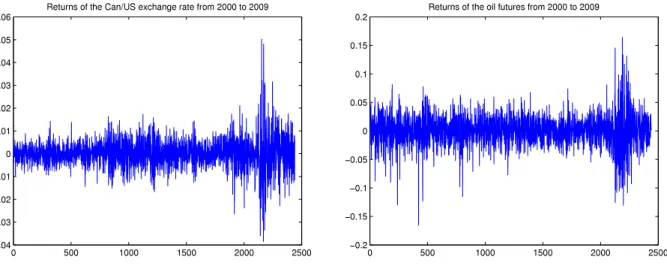
Fig. 1. Plot of the returns for both series from 2000 to 2009.

Table 1

Estimates ofρandν, andp-values of the goodness-of-fit test for the Gaussian and Student copulas, usingN=100 iterations.

Period Gaussian Student

ˆ

ρ p-value (%) ρˆ νˆ p-value (%)

2008–2009 0.435 12 0.444 3.51 71

2005–2009 0.350 53 0.345 5.60 78

2000–2009 0.236 1 0.220 16.7 58

3.4. Ignoring serial dependence

What would have been the effect of ignoring serial dependence? Although most of the resulting estimators would still converge, they might not be regular in the sense of [20,35] and hence goodness-of-fit procedures might be inapplicable. A crucial prior step to inference is thus to test for serial dependence using, e.g., techniques from [19]. This methodology, together with tests of goodness-of-fit proposed in [20], has been implemented in

R

[41].

4. Empirical application

From an economic perspective, dependence between the returns of the Can/US exchange rate and oil prices (NYMEX Oil Futures) is expected. Here, we study this dependence by examining the daily returns data of the two variables over a ten-year period. We investigate three overlapping periods of 2, 5, and 10 years, respectively. These periods are 2008–2009 (493 returns), 2005–2009 (1225 returns), and 2000–2009 (2440 returns). The returns for both series over the entire ten-year period are plotted inFig. 1.

The first step is to test for the presence of serial dependence in the univariate time series (for the three periods); the statisticsInandIn⋆defined in [15] were used to this end. For lags up top

=

6, the tests based onInalmost never reject the

null hypothesis of independence (at the 5% level), while all tests based onI_n⋆reject the same hypothesis.

According to [15], both series exhibit time-dependent conditional variance as in, e.g., GARCH models. Interestingly, classical tests of independence based on the Ljung–Box statistics did not reject the null hypothesis of independence for the exchange rate returns for any of the three periods, though they rejected independence in all cases for the oil futures returns.

Having identified serial dependence in the time-series of both variables, the next step is to attempt to fit a copula-based Markovian model. We chose to test the adequacy of four families: Clayton, Frank, Gaussian, and Student. The zerop-values (calculated withN

=

1000 iterations) for the Clayton and Frank copulas indicate that both families are rejected for every time period.

The corresponding results for the Gaussian and Student copulas appear inTable 1. First, the Student copula systematically exhibits the largestp-value; in each period, it is much larger than the correspondingp-value for the Gaussian copula, which is rejected at the 5% level for the ten-year period. The Student model is thus the best in all cases.

The analysis also confirms the presence of positive dependence between the returns of the two series. The strength of the dependence seems to decrease as the length of the period increases. This may be due to a lack of stationarity for these periods, meaning that the dependence changed between 2000 and 2005 and between 2005 and 2007.Fig. 1supports this hypothesis, at least for the last two years.

Table 2

Estimates ofρandν, andp-values of the goodness-of-fit test for the Student copula, usingN=100 iterations.

Period Student ˆ ρ νˆ p-value (%) 2008–2009 0.444 3.51 71 2005–2007 0.228 39.60 31 2000–2004 0.086 ∞ 37

One can suspect that three different regimes correspond to the periods I: 2000–2004 (1215 returns),

II: 2005–2007 (732 returns), III: 2008–2009 (493 returns).

To test this hypothesis, the same analysis was repeated using only the Student copula. The results are given inTable 2. They confirm the impression that the dependence was different during the three non-overlapping periods, the dependence being much stronger over the last two years, which is often the case during periods of economic and financial stress. However, the surprising result is that for the first period, from 2000 to the end of 2004, the dependence is best modeled by a Gaussian copula (corresponding to a Student copula with an infinite number of degrees of freedom).

Acknowledgments

Funding in support of this work was provided by the Natural Sciences and Engineering Research Council of Canada, the Fonds québécois de la recherche sur la nature et les technologies, Desjardins Global Asset Management, and the Institut de finance mathématique de Montréal. Thanks are due to the Editor, Christian Genest, the Associate Editor and the referees, whose comments led to an improved manuscript. The first author is also grateful to the faculty and staff in the Department of Finance at Singapore Management University for their warm hospitality.

Appendix A. Conditions for mixing

First note that for a stationary Markov chain, the coefficient

α(

n

)

, defined by(15), satisfies

α(

n

)

=

α

{

σ(

U0

), σ(

Un

)

}

. If

general, suppose thatXis a stationary Markov chain with transition

π

and stationary measure

ν

, and letHbe the set of all measurable functionsgso thatE

{

g

(

X0

)

} =

0 and

∥

g

∥

22

=

E

{

g2

(

X0

)

} =

1. Further setTg

(

x

)

=



g

(

y

)π(

x

,

dy

)

, for any

g

∈

H. The maximal correlation

ρ

nis defined by

ρ

n

=

sup

f,g∈H

corr

{

f

(

X0

),

g

(

Xn

)

} =

sup f,g∈H

E

{

f

(

X0

)

g

(

Xn

)

}

.

It follows that for anyf,g

∈

H, and any integern

>

1,

E

{

f

(

X0

)

g

(

Xn

)

} =

E

{

f

(

X0

)

Tg

(

Xn−1

)

} ≤

ρ

n−1

∥

Tg

∥

2

.

Next, note that forg

∈

H,

∥

Tg

∥

2₂

=

E

[{

Tg

(

X0

)

}

2

] =



g

(

y

)(

Tg

)(

x

)π(

x

,

dy

)ν(

dx

)

=

corr

{

Tg

(

X0

),

g

(

X1

)

} ∥

Tg

∥

2

≤

ρ

1

∥

Tg

∥

2

.

As a result,

∥

Tg

∥

₂

≤

ρ

₁, and it follows that for every integern

>

1,

ρ

n

≤

ρ

1

ρ

n−1. Therefore,

ρ

n

≤

ρ

1nfor every integern

≥

1.

In the context of a Markov chainUwith

(

Un−1

,

Un

)

∼

C, as considered previously, set

ρ

C

=

ρ

1. Thus if

ρ

C

<

1, then

ρ

n

goes to zero exponentially fast, and so does

α(

n

)

because

α(

n

)

=

α

{

σ (

U0

), σ (

Un

)

} ≤

1 4

ρ

{

σ (

U0

), σ (

Un

)

} ≤

1 4

ρ

n C

.

Therefore, condition(16)holds true if

ρ

C

<

1. Sufficient conditions for

ρ

C

<

1 to hold are given below. The first result

extends [3, Theorem 3.2].

Proposition 2. Assume c

>

0almost surely on

(

0

,

1

)

2d. Then

ρ

C

<

1if

φ

2 C

= −

1

+



(0,1)2d c2

(

u

, v)

q

(

u

)

q

(v)

d

v

du

<

∞

.

Proof. It follows from [27] that when

φ

_C2

<

∞

, there exists orthonormal sets of functions

(

fk

)

k≥0and

(

gk

)

k≥0onL2

(

q

)

,

f0

=

g0

≡

1, so that for every integersi

,

j

≥

0,



(0,1)2d

φ

2 C

=



i≥1r 2 i, and c

(

u

, v)

=

q

(

u

)

q

(v)



i≥0 rifi

(

u

)

gi

(v)

a.s.

Note thatr0

=

1. Thus iff,g

∈

H, one can find coefficients

α

i,

β

jso that

f

=

∞



i=1

α

ifi a.s.

,

g

=

∞



j=1

β

jgj a.s.

,

∞



i=1

α

2 i

=

1

,

∞



j=1

β

2 j

=

1

.

Hence



(0,1)2d c

(

u

, v)

f

(

u

)

g

(v)

d

v

=

∞



i=1

α

i

β

iri

≤

sup i≥1

|

ri

| ≤

1

.

Given that



i≥1ri2

<

∞

, one has supi≥1

|

ri

| = |

ra

|

for somea

≥

1. Assume that

|

ra

| =

1. Then



(0,1)2d

{

fa

(

u

)

−

raga

(v)

}

2c

(

u

, v)

d

v

du

=

1

−

2ra2

+

r 2 a

=

0

.

Furthermore, the fact thatc

>

0 almost surely implies thatfa

=

λ

af0andga

=

η

ag0, with

λ

a

=

ra

η

a, and

|

η

a

| =

1, which is

impossible because



fa

(

u

)

q

(

u

)

du

=

0 whenevera

≥

1. Hence, one must have

|

ra

|

<

1.

Remark 4. Note that

φ

2_Ccan be defined in terms of the joint law. IfHhas copulaCand densityh, andPhas copulaQ with densityp, then

φ

2 C

= −

1

+



h2

(

_x

,

_y

)

p

(

x

)

p

(

y

)

dydx

.

For the Gaussian copula,

φ

2

C

<

∞

if and only ifA

−

4BMB

⊤_{is positive definite, which is equivalent toM}−1

−

_4B⊤_A−1_B

being positive definite, whereP−1

=

R−₁₁1

+

B⊤Ω−1B,A

=

Ω

+

BPB⊤

=

Ω



2Ω−1

−

R−₁₁1



V,P

=

R11

−

R11B⊤R

−1 11BR11,

M−1

=

_P−1

+

_B⊤_Ω−1_B,M

=

_P

−

_PB⊤_A−1_{BP. We show next that this is always true.}

Because of the properties of the Gaussian distribution, it is sufficient to prove thatQ is positive definite whenR11

=

I,

the identity matrix. SetΣ

=

BB⊤. Observing thatΩ

=

I

−

Σis positive definite, one concludes that all eigenvalues ofΣ are in

[

0

,

1

)

. Next,BP

=

ΩB, soA

=

I

−

Σ2_andBMB⊤

=

_ΩΣ

−

_ΩΣA−1_{ΩΣ. It follows that if}

λ

_{is an eigenvalue ofΣ, then}

(

1

−

λ

2

)

−

4

λ(

1

−

λ)



1

−

λ(

1

−

λ)

1

−

λ

2



=

(

1

−

λ)

3 1

+

λ

is an eigenvalue ofQ. As

λ

∈ [

0

,

1

)

,Q is positive definite. Note that as shown in [3], the tail indices

µ

Land

µ

Uare both

zero whend

=

1 and

φ

2

C

<

∞

, which is equivalent tocbeing square integrable. Therefore,

φ

C2

= ∞

for most interesting

bivariate copulas.

The next result is an extension of [3, Theorem 4.2].

Proposition 3. Assume C admits a density c so that c

(

u

, v)

≥

ϵ

q

(

u

)

q

(v)

almost surely, where q is the density of Q . Then

ρ

C

<

1.

Proof. For any measurable functionsf

,

gso thatf

(

Ut−1

)

andg

(

Ut

)

both have zero mean and unit variance, one has

E

{

f

(

Ut−1

)

g

(

Ut

)

} =

1 2E

{

f 2

(

_U t−1

)

+

g2

(

Ut

)

} −

1 2E

[{

f

(

Ut−1

)

−

g

(

Ut

)

}

2

]

=

1

−

1 2



[0,1]2d

{

f

(

u

)

−

g

(v)

}

2c

(

u

, v)

d

v

du

≤

1

−

ϵ

2



[0,1]2d

{

f

(

u

)

−

g

(v)

}

2q

(

u

)

q

(v)

d

v

du

=

1

−

ϵ.

Hence

ρ

C

≤

1

−

ϵ

.

Example 3. The condition ofProposition 3is verified for one possible extension of the bivariate Farlie–Gumbel–Morgenstern copula family whose density is given, for allu

, v

∈ [

0

,

1

]

d_{, by}

c_θ

(

u

, v)

=

1

+

θ

d



k=1

for some

θ

∈

(

−

1

,

1

)

. It also holds for the Student copula. In the latter case, the ratio is bounded below by a constant times

(

1

+

x⊤R−₁₁1x

/ν)

(ν+d)/2

(

1

+

y⊤R−₁₁1y

/ν)

(ν+d)/2

(

1

+

z⊤R−1z

/ν)

−(ν+2d)/2

,

(A.1) wherez⊤

=

(

x⊤y⊤

)

,xk

=

T_ν−1

(

uk

)

,yk

=

T_ν−1

(v

k

)

,k

∈ {

1

, . . . ,

d

}

. Because

max



x⊤R−₁₁1x

,

y⊤R₁₁−1y



≤

1

+

z⊤R−1z

=

x⊤R−₁₁1x

+

(

y

−

Bx

)

⊤Ω−1

(

y

−

Bx

),

it follows that the ratio(A.1)is bounded below by a constant times

(

1

+

z⊤_R−1_z

)

ν/2_{, which is itself greater than 1. Finally,}

using results from [2], one sees that Frank’s family satisfies the condition ofProposition 3for anyd.

The analog of [3, Theorem 4.3] is given next. It can be used to estimate

ρ

Cnumerically. Before stating the result, let

µ

and

ν

be the measures associated withCandQ, respectively. This notation is required, e.g., for the Clayton and Gumbel–Hougaard families, because neitherProposition 2nor3applies, even whend

=

2, as it is the case in [3].

Proposition 4. Take a partitionPnof sets of the form

Ak

=

d



j=1



kj

−

1 2n

,

kj 2n



,

where k

∈

In

= {

1

, . . . ,

2n

}

d, and let Knbe the2nd

×

2ndmatrix defined by Kn

(

i

,

j

)

=

µ(

Ai

×

Aj

)

−

ν(

Ai

)ν(

Aj

)

for all i, j

∈

In.

Further let Dnbe the diagonal matrix with

(

Dn

)

ii

=

ν(

Ai

)

for all i

∈

In. Finally, let

λ

2nbe the largest eigenvalue of the symmetric

matrix D−n1/2KnD−n1K

⊤

nD

−1/2

n . Then

λ

2n

→

ρ

2Cas n

→ ∞

.

Remark 5. Takingd

=

1, one gets

ν(

Ai

)

=

2−n, so if

ρ

n2is the maximum eigenvalue ofKnKn⊤, then 4 n

ρ

2

n

→

ρ

2

C. Note that

|

ρ

_n

|

is not the maximum eigenvalue ofKnin general, unlessKnis symmetric. So Theorem 4.3 in [3] should be stated with

ρ

n2

as the maximum eigenvalue ofKnKn⊤, instead of saying that

ρ

nis the maximum eigenvalue ofKn.

Proof. As in [3], ifHnis the subset ofHconsisting in functions being constant on the partitionPn, then

∪

n≥1Hnis dense

inH. As a result, lim n→∞_f,sup_g∈H n cov

{

f

(

U0

),

g

(

U1

)

} =

ρ

C

=

sup f,g∈H cov

{

f

(

U0

),

g

(

U1

)

}

.

Fixf,g

∈

Hnand setxi

=

fi

√

ν(

Ai

)

,yi

=

gi

√

ν(

Ai

)

for alli

∈

In. Further defineBn

=

D

−1/2 n KnD −1/2 n . It follows that



(0,1)d f2

(

u

)

q

(

u

)

du

=



i∈In f_i2

ν(

Ai

)

=

1

= ∥

x

∥

2

,



(0,1)d g2

(

u

)

q

(

u

)

du

=



i∈In g_i2

ν(

Ai

)

=

1

= ∥

y

∥

2

,

and hence



(0,1)2d f

(

u

)

g

(v)

{

c

(

u

, v)

−

q

(

u

)

q

(v)

}

d

v

du

=



i∈In



j∈In Kn

(

i

,

j

)

figj

=

x⊤Bny

.

Consequently, sup f,g∈Hn cov

{

f

(

U0

),

g

(

U1

)

} =

sup ∥x∥=∥y∥=1 x⊤Bny

.

The proof is then completed by invoking the fact that ifBis anm

×

mmatrix, then sup

∥x∥=∥y∥=1

x⊤By

=

λ,

where

λ

2_{is the largest eigenvalue ofBB}⊤_.

References

[1] K. Aas, C. Czado, A. Frigessi, H. Bakken, Pair-copula constructions of multiple dependence, Insurance Math. Econom. 44 (2009) 182–198. [2] P. Barbe, C. Genest, K. Ghoudi, B. Rémillard, On Kendall’s process, J. Multivariate Anal. 58 (1996) 197–229.

[3] B.K. Beare, Copulas and temporal dependence, Econometrica 78 (2010) 395–410.

[4] T. Bedford, R.M. Cooke, Vines—a new graphical model for dependent random variables, Ann. Statist. 30 (2002) 1031–1068. [5] D. Berg, Copula goodness-of-fit testing: an overview and power comparison, Europ. J. Finance 15 (2009) 675–701.

[6] R.C. Bradley, Basic properties of strong mixing conditions, a survey and some open questions, Probab. Surv. 2 (2005) 107–144. [7] X. Chen, Y. Fan, Estimation of copula-based semiparametric time series models, J. Econometrics 130 (2006) 307–335.

[8] X. Chen, Y. Fan, Estimation and model selection of semiparametric copula-based multivariate dynamic models under copula misspecification, J. Econometrics 135 (2006) 125–154.

[9] F.X. Diebold, T.A. Gunther, A.S. Tay, Evaluating density forecasts with applications to financial risk management, Int. Econ. Rev. 39 (1998) 863–883. [10] P. Doukhan, J.-D. Fermanian, G. Lang, An empirical central limit theorem with applications to copulas under weak dependence, Stat. Inference Stoch.

Process. 12 (2009) 65–87.

[11] P. Duchesne, R. Roy, Robust tests for independence of two time series, Statist. Sinica 13 (2003) 827–852. [12] R. Durrett, Probability: Theory and Examples, second ed., Duxbury Press, Belmont, CA, 1996.

[13] P. Embrechts, A.J. McNeil, D. Straumann, Correlation and dependence in risk management: properties and pitfalls, in: Risk Management: Value at Risk and Beyond (Cambridge, 1998), Cambridge Univ. Press, Cambridge, 2002, pp. 176–223.

[14] J.-D. Fermanian, M. Wegkamp, Time-dependent copulas, J. Multivariate Anal. 110 (2012) 19–29.

[15] C. Genest, K. Ghoudi, B. Rémillard, Rank-based extensions of the Brock, Dechert, and Scheinkman test, J. Amer. Statist. Assoc. 102 (2007) 1363–1376. [16] C. Genest C., K. Ghoudi, L.-P. Rivest, A semiparametric estimation procedure of dependence parameters in multivariate families of distributions,

Biometrika 82 (1995) 543–552.

[17] C. Genest, R.J. MacKay, Copules archimédiennes et familles de lois bidimensionnelles dont les marges sont données, Canad. J. Statist. 14 (1986) 145–159.

[18] C. Genest, R.J. MacKay, The joy of copulas: bivariate distributions with uniform marginals, Amer. Statist. 40 (1986) 280–283. [19] C. Genest, B. Rémillard, Tests of independence and randomness based on the empirical copula process, Test 13 (2004) 335–369.

[20] C. Genest, B. Rémillard, Validity of the parametric bootstrap for goodness-of-fit testing in semiparametric models, Ann. Inst. H. Poincaré Probab. Statist. 44 (2008) 1096–1127.

[21] C. Genest, B. Rémillard, D. Beaudoin, Goodness-of-fit tests for copulas: a review and a power study, Insurance Math. Econom. 44 (2009) 199–213. [22] K. Ghoudi, B. Rémillard, Empirical processes based on pseudo-observations. II, the multivariate case, in: Asymptotic Methods in Stochastics, in: Fields

Inst. Commun., vol. 44, Amer. Math. Soc., Providence, RI, 2004, pp. 381–406.

[23] E. Giacomini, W. Härdle, V. Spokoiny, Inhomogeneous dependence modeling with time-varying copulae, J. Bus. Econom. Statist. 27 (2009) 224–234. [24] D. Guégan, J. Zhang, Change analysis of a dynamic copula for measuring dependence in multivariate financial data, Quant. Finance 10 (2010) 421–430. [25] A. Harvey, Tracking a changing copula, J. Empir. Finance 17 (2010) 485–500.

[26] E. Kole, K. Koedijk, M. Verbeek, Selecting copulas for risk management, J. Banking Finance 31 (2007) 2405–2423. [27] H.O. Lancaster, The structure of bivariate distributions, Ann. Math. Statist. 29 (1958) 719–736.

[28] A.W. Marshall, I. Olkin, Families of multivariate distributions, J. Amer. Statist. Assoc. 83 (1988) 834–841. [29] A.J. McNeil, Sampling nested Archimedean copulas, J. Statist. Comp. Simul. 78 (2008) 567–581.

[30] A.J. McNeil, J. Nešlehová, Multivariate Archimedean copulas,d-monotone functions andℓ1-norm symmetric distributions, Ann. Statist. 37 (2009) 3059–3097.

[31] M. Mesfioui, J.-F. Quessy, Dependence structure of conditional Archimedean copulas, J. Multivariate Anal. 99 (2008) 372–385. [32] A.J. Patton, Modelling asymmetric exchange rate dependence, Int. Econ. Rev. 47 (2006) 527–556.

[33] A.J. Patton, Copula-based models for financial time series, in: Handbook of Financial Time Series, Springer, Berlin, 2009, pp. 767–785. [34] A.J. Patton, A review of copula models for economic time series, J. Multivariate Anal. 110 (2012) 4–18.

[35] B. Rémillard, Validity of the parametric bootstrap for goodness-of-fit testing in dynamic models, Technical report, SSRN Working Paper Series No 1966476, 2011.

[36] B. Rémillard, A. Hocquard, N. Papageorgiou, Option pricing and dynamic discrete time hedging for regime-switching geometric random walk models, Tech. Report, SSRN Working Paper Series No 1591146, 2010.

[37] B. Rémillard, N. Papageorgiou, Modelling asset returns with Markov regime-switching models, Tech. Report 3, DGAM-HEC Alternative Investments Research, 2008.

[38] E. Rio E., Théorie Asymptotique Des Processus aléatoires Faiblement Dépendants, Springer, Berlin, 2000. [39] A. Sklar, Fonctions de répartition àndimensions et leurs marges, Publ. Inst. Statist. Univ. Paris 8 (1959) 229–231.

[40] R.W.J. van den Goorbergh, C. Genest, B.J.M. Werker, Bivariate option pricing using dynamic copula models, Insurance Math. Econom. 37 (2005) 101–114.

[41] J. Yan, I. Kojadinovic, The copula package,http://cran.r-project.org/web/packages/copula/copula.pdf, 2009.

[42] W. Yi, S.S. Liao, Statistical properties of parametric estimators for Markov chain vectors based on copula models, J. Statist. Plann. Inf. 140 (2010) 1465–1480.