University of Pennsylvania
ScholarlyCommons
Finance Papers Wharton Faculty Research
2-22-2016
Good-Specific Habit Formation and the
Cross-Section of Expected Returns
Jules van Binsbergen
University of Pennsylvania
Follow this and additional works at:https://repository.upenn.edu/fnce_papers
Part of theFinance Commons, and theFinance and Financial Management Commons
This paper is posted at ScholarlyCommons.https://repository.upenn.edu/fnce_papers/246 For more information, please [email protected].
Recommended Citation
van Binsbergen, J. (2016). Good-Specific Habit Formation and the Cross-Section of Expected Returns.The Journal of Finance,
Good-Specific Habit Formation and the Cross-Section of Expected
Returns
Abstract
I study asset prices in a general equilibrium framework in which agents form habits over individual varieties of goods rather than over an aggregate consumption bundle. Goods are produced by monopolistically
competitive firms whose elasticities of demand depend on consumers' habit formation. Firms that produce goods with a high habit level relative to consumption have low demand elasticities, set high prices for their product, have low expected returns on their stock and have low asset pricing betas and stock return volatilities. I find supportive evidence for these predictions in the data.
Disciplines
Good-Specific Habit Formation and the Cross-Section
of Expected Returns
∗Jules H. van Binsbergen
Stanford GSB
†This version: June 2009
Abstract
I study the cross-section of expected stock returns in a general equilibrium framework in which agents form habits over individual varieties of goods as opposed to over a composite consumption good. Goods are produced by monopolistically competitive firms whose income and price elasticities of demand depend on the habit formation of the consumers. Firms who produce goods with a low consumption surplus ratio earn low expected returns because their income and price elasticities of demand are low. By sorting firms in portfolios based on their consumption surplus ratio or based on their recent price setting behavior, I find a return spread of 5%, that can not be explained by the CAPM or by the Fama French three factor model.
∗First version: November 2007. This paper was previously circulated under the title “Deep Habits
and the Cross-Section of Expected Returns”. I thank Hengjie Ai, Ravi Bansal, Michael Brandt, Alon Brav, Craig Burnside, John Campbell, John Cochrane, Darrell Duffie, Jesus Fernandez-Villaverde, Simon Gervais, John Graham, Cam Harvey, Dirk Jenter, Ralph Koijen, Rich Matthews, Juan Rubio Ramirez, David Robinson, Tano Santos, Stephanie Schmitt-Grohe, Ken Singleton, Martin Uribe, Vish Viswanathan, seminar participants at Barclays Global Investors, Carnegie Mellon, Chicago, Columbia, Duke, the Federal Reserve Board, Harvard, MIT Sloan, Kellogg, NYU Stern, Princeton, Stanford GSB, UCLA, USC, Wharton, Yale School of Management, the EFA 2008 meetings, the AFA 2009 meetings, and in particular Anamar´ıa Pieschac´on for helpful discussions and comments. All remaining errors are my own.
1
Introduction
Explaining the cross-section of expected returns lies at the core of asset pricing. Even though habit formation models have proven successful in explaining some of the key properties of the time series of expected returns,1 explaining the cross-section of expected returns seems more challenging.2 So far, in the asset pricing literature, it is common to assume that households derive utility and form their habits from the consumption of a single aggregate good.3 In this paper, I study asset prices in an economy where households form their habits not over a single aggregate good, but over individual varieties of goods produced by monopolistically competitive firms. Both the income elasticity and the price elasticity of demand of each monopolist is time-varying and proportional to the consumption surplus ratio for the monopolist’s good. Firms that produce goods with a low consumption surplus ratio, that is, a consumption level close to the habit level, earn low expected returns because they face low income and price elasticities of demand, making their profits less susceptible to real aggregate shocks. Furthermore, the low price-elasticity of demand will lead to high markups.
The main mechanism generating the difference in expected returns is relatively straightforward. Consumers are highly averse to scaling back on goods for which the consumption level is close to the habit level, which implies that both the income elasticity and price-elasticity of demand for such goods is low. In response to negative aggregate shocks, the demand for goods with a low consumption surplus ratio will remain relatively strong, due to the low income elasticity of demand. Furthermore, the relative prices of goods with a low consumption surplus ratio are high, and increase in response to negative aggregate shocks.4 These price increases lower the exposure of the producers to such systematic shocks resulting in a lower risk premium. In contrast, the producers of goods with a high consumption surplus ratio, that is, a consumption level that is far way from the habit level, are faced with a negative relative price change in addition to the negative aggregate productivity shock.
To illustrate the generality of the mechanism that generates the difference in expected returns, I present two versions of the model, a endowment-based model without production factors and a production-based model. In the endowment model there are two types of shocks, one systematic shock to the aggregate habit-adjusted consumption level and
1See Abel (1990), Constantinides (1990), Heaton (1995), Jermann (1998), Campbell and Cochrane (1999)
and Campbell and Cochrane (2000)
2See for example Lettau and Wachter (2007) and Santos and Veronesi (2006)
3Notable exceptions are Ait-Sahalia, Parker, and Yogo (2004), Yogo (2006), Gomes, Kogan, and Yogo
idiosyncratic demand shocks to the habit stock of each firm. Whereas the systematic shock drives the aggregate consumption surplus ratio, the risk free rate and the equity risk premium, the idiosyncratic demand shock drives the cross-sectional variation of consumption surplus ratios in the model. As the consumption surplus ratios determine the amount of exposure to systematic shocks, this cross-sectional variation drives the cross-section of expected returns. In the production-based model, instead of focusing on demand shocks, the cross-section of consumption surplus ratios (and hence of expected returns) is driven by productivity shocks. The main purpose of presenting these two models in parallel is to stress that regardless of the source of idiosyncratic variation, the implications are the same: firms with low consumption surplus ratios earn low expected returns.
In both models each good is produced by a single monopolistically competitive firm. Ex ante all firms are identical but as shocks realize, firms differ with respect to the habit stock for the goods they produce. In this setup, the unconditional CAPM beta of each firm, that is, the beta with respect to the market portfolio, equals one and the unconditional risk premia of all firms are equal. However, each firm’s risk premium is time-varying and dependent on the habit stock for its good relative to the habit stocks of all other goods in the economy.
I confirm the predictions of the model empirically in two ways. First I use quantity data between 2001 and 2008 from the Bureau of Economic Analysis on shipments for 423 NAICS industries. I construct consumption surplus ratios for each industry and sort firms into portfolios based on the consumption surplus ratio of their industry. This sorting generates an expected return spread of 6% that cannot be explained by the CAPM or the Fama French three factor model. Secondly, I use data from the industry level Producer Price Index (PPI) program. The PPI measures the average change over time in the selling prices received by domestic producers for their output. By sorting firms into quintile portfolios based on their recent percentage price changes, I find that firms that recently increased their prices earn lower expected returns than firms that recently decreased their prices, generating an annual expected return spread of 6 percent that can neither be explained by the unconditional Capital Asset Pricing Model (CAPM) nor by size, book-to-market and momentum effects.
In other words, when sorting firms into quintiles based on their recent pricing behavior a large premium can be generated. The raw (unadjusted) average return difference between quintile 1 (firms with the largest price decreases) and quintile 5 (firms with the largest price increases) equals 0.54 percent per month. Part of this premium can be explained by the CAPM and the loading of the DMI portfolio (Deflationary-minus-Inflationary), on the market portfolio is positive. The pricing error relative to the unconditional CAPM is however still significant. When including the other Fama-French factors and momentum, the pricing
error further increases, as firms with recent price decreases earn high expected returns, but load negatively and significantly on the book-to-market factor.
My approach stands in contrast to several recent papers that employ cross-sectional variation on the production side of the economy to explain characteristics of the cross-section of expected returns.5 In the deep habits model the cross section of expected returns is purely driven by the habit formation of consumers and I assume that all firms have access to the same production technology to produce their good. However, it is important to stress that I view the deep habits model not as a competing explanation for the cross-section of expected returns but rather as the demand-side complement to the existing literature that employs cross-sectional differences in the production technologies of firms to explain the cross-section of expected returns.
Apart from the cross-sectional implications, I also study the aggregate time series properties of the model. The endowment model performs well in matching the aggregate moments. The production-based model performs equally well as the one-sector habit formation model with production as in Jermann (1998). The model matches the aggregate risk premium, the level of the riskfree rate and the volatility of output growth, investment growth and consumption growth. Furthermore, by imposing persistence for the evolution of the habit stock, the model also matches the low volatility of the riskfree rate, whereas in the one-sector habit formation model with production this volatility seems several factors too high. However, the volatility of dividend growth in Jermann’s model seems too low, whereas the deep habits model generates volatile dividend growth rates close to those of firms’ net payout, as opposed to per share dividends.6 The production-based model also seems to perform poorly with respect to the conditional moments of the financial variables. In particular, the variation in the price dividend ratio seems mainly driven by variation in expected dividend growth rates and not by variation in expected returns, as, in the model, the latter only has limited variation.
The main feature of the model is that households have preferences and form habits over individual goods as opposed to over a single aggregate consumption bundle. There are two special cases when the stochastic discount factor simplifies to the standard habit formation model with a single aggregate good: (i) when goods are perfect substitutes and (ii) when there is perfect symmetry between goods (and firms). When goods are perfect substitutes consumers only care about the size of the aggregate consumption bundle and not about its composition. This seems an unlikely characteristic of household preferences. With perfect
symmetry between goods and firms, I mean that all firms face the same productivity shocks resulting in the same habit level for all goods.7 In this case, the model implies that all relative prices are constant over time. However, empirically we do observe time variation in relative prices. Good-specific habits endogenously generate such time variation in prices. Given that habit formation models have proven successful in explaining the level and time variation of aggregate risk premia, it seems natural to study the interaction between relative prices and the cross-section of expected returns in a good-specific habits framework.
The implications of multiple goods for asset prices has also been explored by Ait-Sahalia, Parker, and Yogo (2004), Yogo (2006) and Gomes, Kogan, and Yogo (2006). Ait-Sahalia, Parker, and Yogo (2004) argue for the distinction between luxury goods and basic goods. Households are more risk averse with respect to the consumption of basic goods due to the presence of a subsistence point for such goods. Using data on the consumption of luxury goods, they find that the risk aversion implied by luxury good consumption is more than an order of magnitude less than that implied by national accounts data which mostly reflects basic consumption. Yogo (2006) and Gomes, Kogan, and Yogo (2006) argue for the distinction between durable goods and non-durable goods and find that the producers of durable goods earn higher expected returns, as the demand for durable goods is more pro-cyclical. The stocks of producers of durable goods therefore carry more systematic risk. None of these papers, however, consider good-dependent habit formation and the interaction between the price-setting behavior of producers and the expected returns on their stock.
My model also relates to the recent literature on the cross-section of expected returns and product market competition. Hou and Robinson (2006) show that US firms in the quintile of the most competitive industries earn annual returns that are nearly 4% higher than those of similar firms in the quintile of the most concentrated industries. The market power that Hou and Robinson (2006) consider is related to the price setting behavior that I study in this paper. That being said, in my model, the elasticity of substitution between all goods is equal, and therefore the competition between all firms is equal. Furthermore, in my model, low expected returns are not a unconditional characteristic of an industry or firm but are a consequence of the current low income and price elasticities of demand faced by a particular firm or industry, which is time-varying. When I construct the quintile portfolios, I indeed find that firms (and industries) frequently rotate across quintiles.8 In contrast, firm
7Even though the stochastic discount factor simplifies to the standard habit formation discount factor
with a single aggregate good, the firm’s optimization problem still takes the habit formation of the consumers into account, resulting in different cash flow dynamics. I further explore the perfect symmetry case when assessing the time series properties of the model.
sorts based on each industry’s Herfindahl-Hirschman Index (HHI), as in Hou and Robinson (2006), can be used to generate a spread in expected returns up to several decades into the future. By including the return spread on the HHI portfolios as a factor, I find that the DMI portfolio that I construct does not significantly load on the HHI factor, both in the economic and the statistical sense.9
To my knowledge this is the first paper that explores the implications of good-dependent habits and producer prices on asset prices. One obvious question that comes to mind is how coarse the classification of varieties should be. With varieties of goods, I have in mind an environment in which consumers form habits over narrowly defined categories of goods, such as clothing, vacation destinations, music and cars. The advantage of defining habits over categories of goods as opposed to over specific goods within categories, is that household expenditure on categories of goods general goes up as income increases, that is, they behave as normal goods. Individual goods within categories, on the other hand, may be inferior goods, that is, expenditure on these goods decreases as income increases.
The idea that households form their habits over individual varieties of goods has recently been introduced in the macroeconomic literature by Ravn, Schmitt-Grohe, and Uribe (2006) who propose to call this type of habit formation ”deep” habits. These authors show that the deep habits model can help to explain several interesting macroeconomic empirical facts. In particular, they show that expansions in output driven by preference shocks, government-spending shocks, or productivity shocks are accompanied by declines in mark-ups. This implication of the deep habits model is in line with the extant empirical literature, which finds mark-ups to be counter-cyclical (Rotemberg and Woodford (1999)). Product-specific habit formation also has a long tradition in the marketing literature, starting with Guadagni and Little (1983). This literature uses the term ”loyalty variable”. This loyalty variable measures how hooked consumers are on a given firm’s product and it is measured as a weighted average of past sales. It therefore closely resembles the notion of habits in the economics and finance literature. This literature also widely discusses the importance of brand and product loyalty for firm valuation. In this paper, I argue that product loyalty does not only increase firm value due to higher cash flows, but also due to a lower discount factor.
2
A Simple Model without Production Factors
2.1
Households, Varieties and Preferences
Following Ravn, Schmitt-Grohe, and Uribe (2006), the economy consists of a representative household and a continuum of goods, also called varieties, with an aggregate mass of one. Goods are produced by monopolistically competitive firms. As such, each good is produced by a single monopolist and there exists a one-to-one mapping between varieties and firms. I assume that the representative household’s preferences are described by the utility function:
E0 ∞ X t=0 βtX 1−γ t 1−γ (1)
where Xt is the aggregate level of habit-adjusted consumption for t ∈ {0,1}. The level of
aggregate habit-adjusted consumption, Xt is defined as:
Xt= 1 Z 0 (Cit−θSit)1 −1 η di 1 1−1η (2)
where Cit is the level of consumption of variety i, and Sit is the habit of variety i, which
is known at time t−1 apart from a preference shock. The parameter η is the elasticity of substitution between the varieties of goods as in Dixit and Stiglitz (1977) and the parameter θ determines the time non-separability of the preferences. Assume that the habit for good i in period t is given by:
Sit= (ρSi,t−1+ (1−ρ)Ci,t−1) exp(εit) (3)
where εit ∼ N(−12σs2, σs2) represents the habit or demand shock. This demand shock is
uncorrelated across firms, and therefore averages out when we aggregate over habit levels.10 Let Pit denote the price charged by the producer of good i for one unit of good i at time
t. For a given level of aggregate habit-adjusted consumption Xt, the household chooses its
consumption bundle to minimize total expenditure
min 1 Z 0 PitCitdi (4) 10I modelε
it as a multiplicative shock instead of an additive shock for the sole purpose of ensuring that
subject to equation 2. This optimization results in the following demand function: Cit= Pit Pt −η Xt+θSit (5)
where Pt is an aggregate price index given by Pt =
1 R 0 P1−η it di 1 1−η . The consumption of varietyiis decreasing in its relative pricepit ≡ PPitt, increasing in the level of aggregate
habit-adjusted consumption Xt, and, for θ > 0, increasing in the habit stock for consumption of
variety i. As both terms on the righthand side of equation 5 are positive, the consumption surplus ratio for each good is strictly positive.
2.2
Price and Income Elasticities
The price (P) elasticity of demand (C) for good i at time t measures the percentage change of the demand for good i when changing the price of good i by one percent while holding the habit level and the aggregate price level constant:
ǫC,Pit = ∂lnCit ∂lnPit = ∂ln Pit Pt −η Xt+θSit ∂lnPit =−η Cit−θSit Cit . (6)
Note that this elasticity is time-varying and proportional to the consumption surplus ratio for good i.
Furthermore, the elasticity of demand (C) for firmi with respect to the aggregate habit-adjusted consumption (X), which ceteris paribus (c.p.) measures the percentage change of demand in response to a one percent change in Xt, is given by:
ǫC,Xit = ∂lnCit ∂lnXt = ∂ln Pit Pt −η Xt+θSit ∂lnXt = Cit−θSit Cit . (7)
I will refer to this elasticity as the income elasticity of demand even though strictly speaking it is not the elasticity with respect to income but the elasticity with respect to aggregate habit-adjusted consumption. This income elasticity is equal to the consumption surplus ratio and it provides a parsimonious explanation for why firms with a low consumption surplus ratio earn low expected returns. The profits of firmican be written as Φit =Cit(Pit−MCit).
as:
∆ ln Φit+1 = ∆ lnCit+1+ ∆ ln (Pit+1−MCit+1) (8)
First assume for now that prices and costs are constant. In this case, profits only vary over time due to changes in the quantity soldCit. With a slight abuse of notation, the covariation
between the log stochastic discount factor and log changes in profits can then be written as:
−γcov (∆ ln Φit+1,∆ lnXit+1) ≈ −γcov Cit−θSit Cit ∆ lnXit+1,∆ lnXit+1 (9) = −γ Cit−θSit Cit var (∆ lnXit+1) (10)
The equation above shows that firms with a low consumption surplus ratio have a demand for their product with a low income elasticity. Hence, such firms have a lower exposure to aggregate shocks, that is, shocks to aggregate habit-adjusted consumption Xt. Because
shocks to aggregate habit adjusted consumption drive shocks to the stochastic discount factor, such firms have a lower risk premium.
In the derivation above I have assumed that quantities are free to adjust and that prices remain constant. Now consider the other extreme when quantities are not free to adjust. In this case, product prices will have to adjust in equilibrium.11 Suppose, for example, that all firms face an equally large percentage productivity shock. Suppose further that firms can not unwind this negative productivity shock by employing more input factors to production, which implies an equally large negative output shock. In this case, firms with a low consumption surplus ratio are less risky due to their smaller price elasticity of demand. The price elasticity of demand of each firm is proportional to the consumption surplus ratio. As a consequence, if the percentage change of the quantities is the same for all goods, the goods with the smallest consumption surplus ratio will have the largest product price change. Because the price elasticity of demand is so small, small quantity changes imply large price changes. As a consequence, in response to a negative (aggregate) productivity shock, the product prices of goods with a low consumption surplus ratio will increase, which serve as a hedge against these negative productivity shocks. Because the aggregate price index is normalized to one, firms with a high consumption surplus ratio will face a real price decrease in addition to the negative productivity shock.
The latter result can also be understood in terms of markups. Note that the deep habits model endogenously generates countercyclical markups. For all firms, these countercyclical
11One particular example when quantities are not free to adjust is the presence of adjustment costs to the
markups serve as a hedge against aggregate income shocks. Even though aggregate demand goes down, the markup increase will compensate for this loss in demand. However, the argument presented in the previous paragraph indicates that markups go up more for firms with a low consumption surplus ratio thereby creating cross-sectional differences in expected returns. As such, the differences in expected returns are driven by both income- and price-elasticity effects.
2.3
Competitive Markets
I assume that each variety of good is offered by both a monopolistically competitive firm as well as by a competitive market.12 I assume that the monopolistically competitive firms own a technology that allows them to offer their product at a lower marginal cost than the competitive market can. This assumption bounds from above the price that each monopolist is willing to set. If the monopolist charges too high a price, the competitive market takes over. If such a competitive market would not exist, there is an incentive for firms to charge an infinitely large price for their product and exploit the habit formation of the consumers in this way.13
2.4
Firms
Each monopolistically competitive firm produces its product at a fixed marginal cost MC and maximizes its real value subject to the demand function and the habit process, resulting in the following Lagrangian:
Li =E0 " ∞ X t=0 Xt X0 −γ (Pit−M C) Pt Cit+νit p−η it Xt+θSit−Cit +ζit{(ρSit+ (1−ρ)Cit) exp(εit+1)−Sit+1} !# (11)
12I thank V.V. Chari and Larry Christiano for suggesting this market structure to me.
13Ravn, Schmitt-Grohe, and Uribe (2006) assume that consumers have a taste for product variety and
that consumers are allowed to drop a certain variety from the consumption bundle if the monopolist would charge too high a price. The implication of this assumption is the same, which is that the price charged by the monopolist is bounded from above.
Each firm i takes Xt and Pt as given. The variable Sit is an endogenous state variable.
Taking first order conditions with respect to Cit, Sit and pit we obtain:
[Cit] : Pit−MC Pt −νit+ (1−ρ)ζit = 0 (12) [Sit] : Et Λt+1 Λt (θνit+1+ρζit+1) =ζit (13) [pit] : Cit−ηνitp −η−1 it Xt= 0. (14)
The first of these three equations balances the marginal cost and benefit from a one unit increase of consumption. The Lagrange multiplier νit measures the value of an additional
unit of demand in this period. This value is equal to the real markup plus the present-value of having (1−ρ) additional units of habit in the next period. The present value of having one additional unit of habit in the next period equals ζit, so the value of having 1−ρ such
units equals (1−ρ)ζit.
The second equation balances the marginal costs and benefits of increasing the habit of the households, which due to the persistence of the habit stock is a dynamic tradeoff. An additional unit of habit in this period leads to ρ additional units of habit in the next period. Having an additional unit of habit allows the firm to raise prices as the price elasticity of the consumers’ demand is now lower, generating an additional revenue equal to θνit+1. Note that the optimal price response depends on the time non-separability of the consumers’ preferences measured byθ. Finally, the third equation equates the marginal costs and benefits of changing the price of the good by one unit.
2.5
Endowment Dynamics
Instead of modeling the consumption process for each firmi, I postulate that log aggregate habit-adjusted consumption follows a persistent AR(1) process around a deterministic time trend g in the spirit of Jermann (1998):
xt ≡ ln(Xt) =gt+zt (15)
zt = ̺zzt−1 +εzt (16)
where εzt is the systematic shock in the economy, which is uncorrelated to the idiosyncratic
demand shocks in the habit process εit. I assume, that the shock εzt is normally distributed
surplus ratio is low, the volatility of the stochastic discount factor is high:
εzt∼N(0,exp(−bxt−1)σz2) (17)
This is consistent with Campbell and Cochrane (1999) who consider one composite consumption good and model log consumption growth as a homoskedastic i.i.d. process, implying that zt has time-varying volatility inversely related to the consumption surplus
ratio. Both in my framework as well as in Campbell and Cochrane (1999), this time-varying volatility drives the variation in risk premia.
I wish to stress that time-varying volatility does not play an important role in generating a cross-sectional spread in expected returns, which is the main topic of this paper. However, it does play an important role in matching the time series properties of the riskfree rate and the equity risk premium to the data as further explained in Section 2.8.3.
2.6
Calibration
Define the set of parameters Θ as:
Θ≡ {β, γ, η, g, ̺z, ρ, θ, σz, σs, MC} (18)
Table 8 lists the calibrated parameters. The risk aversion parameter γ is calibrated to a value of 8. The deterministic log growth rate of the economy is calibrated to 0.4% per quarter as in Jermann (1998). The subjective discount factor β is calibrated to 1.01 such that β∗
= β(exp(g))1−γ
equals 0.98. I calibrate the elasticity of substitution to a value of 5.3, as in Ravn, Schmitt-Grohe, and Uribe (2006). I set the time-separability parameter θ equal to 0.8 following Jermann (1998) and Constantinides (1990). I set the volatility of the endowment shockσz to 2.65% and the volatility of the idiosyncratic demand shock to 7%. I
normalize the marginal cost MC of each firm to 1.
2.7
Solution Method
Each firm takes the processes for Xt and Pt as given. The process for Xt (or equivalently
zt) is exogenous. The value of Pt, on the other hand, is a function of the cross-sectional
distribution of prices Pit, which in turn depends on the whole cross-sectional distribution of
state variable by the average habit level in the economy given by: St=
Z 1
0
Sitdi (19)
leads to a highly accurate solution. I demonstrate this in the following way. The price-setting behavior Pit of each firm conditional on a guessPt∗ should be such that the aggregate
price index level Pt =
1 R 0 P1−η it di 1−1η , is equal to P∗
t. I solve the model using perturbation
methods as further described in Appendix A, using the following steps:
1. I solve the model setting the volatility of the idiosyncratic demand shocks to zero: σ2
s = 0. Under appropriate conditions for the starting values of the state variables, this
implies that all firms are identical. Because now all firm-specific variables are equal, aggregation over firms is straightforward, and the model can easily be solved for one representative firm.
2. I then solve the problem for firm iincluding the idiosyncratic demand shock and take the process for the aggregate price level from step 1. That is, the guess P∗
t equals the
aggregate price level from step 1.
3. I simulate at each point in time a cross-section of firms using the solution found in step 2, and compute at each point in time the aggregate price index levelPt=
1 R 0 P1−η it di 1 1−η
implied by this cross-sectional distribution.
4. I compare the aggregate price index level Ptfrom step 3 with the aggregate price index
level P∗
t and find that they have almost identical means, identical standard deviations
and a correlation of 0.999.
2.8
Simulation Results
The simulation results are summarized in Table 2 and Figures 1, 2 and ??. The results can be summarized as follows. First, the model generates an expected return spread of 4% which can be generated by sorting firms either based on their consumption surplus ratios or on their relative prices. Secondly, the model seems to be able to match several key characteristics of both real and financial variables, such as the dynamics of aggregate consumption growth, the riskfree rate and the equity risk premium. In the following subsections, I will present these results in detail.
2.8.1 The Cross-Section of Expected Returns
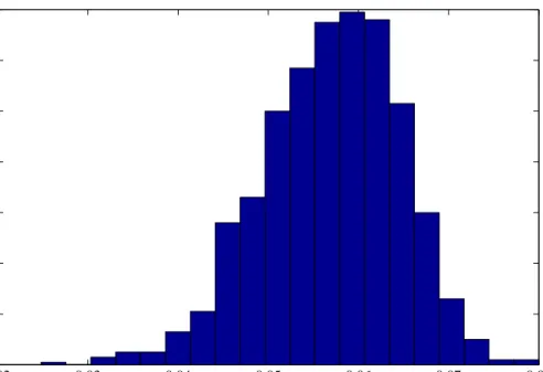
The main result of the paper is summarized in Figures 1 and 2. I simulate a cross-section of 1000 firms over time. Figure 1 plots a histogram of the cross-section of annualized expected excess returns in a period where bothztand the aggregate habit levelSt are at their average
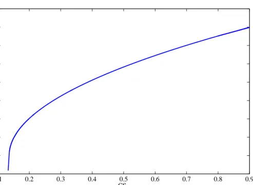
values. The histogram shows that with the current calibration, the model generates an annual expected return spread of 4%. Figure 2 takes the same cross-section of expected excess returns and plots them against the cross-section of consumption surplus ratios. The figure shows that there is a positive relationship between the consumption surplus ratio of firm iand the expected excess return of firm i. Firms with a low consumption surplus ratio have low income and price elasticities of demand and are therefore less risky.
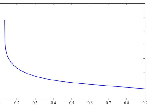
Finally, Figure 3 takes the same cross-section of consumption surplus ratios, and plots them against the cross-section of relative prices pit = PPitt. The figure shows that there is a
negative relationship between the consumption surplus ratio of firm i and the relative price it charges for its product. Firms with a low consumption surplus ratio have a low price elasticity of demand and therefore set high a price for their product. As the relationship between consumption surplus ratios and expected returns is positive and the relation between consumption surplus ratio and relative prices is negative, the relationship between expected returns and prices is negative. That is, an expected return spread can be generated by sorting firms into portfolios based on their price setting behavior.
2.8.2 Real Variables
In this version of the model there is no investment. Hence aggregate real consumption equals aggregate real production (GDP). In the data, the quarterly volatility of aggregate consumption growth is 0.6% and the quarterly volatility of GDP growth equals 1%. Without investment, my model can either match the volatility of aggregate consumption growth or the volatility of aggregate GDP growth, not not both. I calibrate the volatility of the aggregate shock εz such that in the model the volatility of aggregate consumption (production) growth
equals 0.7%.
The model generates a countercyclical aggregate markup of prices over marginal costs with an average of 25% and a time series unconditional standard deviation of 8.8%. The model also gives predictions for the volatility of quantity growth of individual firms. In the model, the quarterly volatility of ∆ln(Cit) equals 5.9%, about ten times as high as aggregate
2.8.3 Risk Free Rate
The model is also able to match the volatility of the riskfree rate. Campbell and Cochrane (1999) model their habit dynamics such that the riskfree rate is constant within a consumption-based framework. Jermann (1998) and Boldrin, Christiano, and Fisher (2001) present production-based models with standard habit dynamics, but conclude that the volatility of the riskfree rate is too high. The habit dynamics in my model are standard and habits are equal to an exponentially weighted sum of past consumption levels. The mechanism through which I match the volatility of the riskfree rate is through the time-varying volatility of the z-process, which is modeled such that when times are bad and the consumption level is close to the habit level, the volatility of the stochastic discount factor is high. This is consistent with Campbell and Cochrane (1999), but the mechanism is slightly different. In Appendix C I derive the dynamics of the riskfree rate and show that:
rf t ≈ −logβ+γg− 1 2γ 2σ2 z +γ γbσz2−(1−ρ) zt
The average riskfree rate is equal to−logβ+γg−12γ2σ2
z. The exposure of the risk free rate
to the exogenous state variable zt is given by γ(γbσz2−(1−ρ)). When the parameter b is
calibrated to a value of (1−ρ)
γσ2
z , the riskfree rate is constant. In this case, the precautionary
savings motive γ2bσ2
zzt and the expected growth of zt, represented by the term (1−ρ)zt
cancel each other out.
2.8.4 Stock Returns
The annual aggregate equity risk premium equals 5.8% in the model, which is slightly higher than the 5.5% in the data. With the current calibration, the model underestimates the volatility of the return on the aggregate stock market. The annual stock market volatility equals 14.1%, slightly lower than the 17.8% in the data. The volatility of annual aggregate earnings growth equals 22.5% in the model and 22.1% in the data.
The time variation in the volatility of zt also drives the large variation in the conditional
equity risk premium. The quarterly volatility of the conditional risk premium equals 0.4%, which is higher then the quarterly volatility of the riskfree rate, which equals 0.3%. The risk premium is also highly persistent. These facts seems consistent with the recent evidence on return predictability.14
The model also gives predictions for the volatility of the stock returns and earnings growth of individual firms. The annual volatility of each firm’s stock is 32% and the volatility
of earnings growth is 42% which are both close to the data in the CRSP/COMPUSTAT database. The model thus generates substantial idiosyncratic volatility generated by idiosyncratic demand (habit) shocks.
3
A Model with Production
In the previous section I have presented a parsimonious model without production factors. The marginal cost of each firm was constant and firms could produce as many products at this marginal cost as desirable. I now present a production-based economy which generates similar results to the model presented in the previous section.
3.1
Households
The representative household’s preferences are described by the utility function: E0
∞
X
t=0
βtU(Xt, ht) (20)
where Xt is the level of habit-adjusted consumption and ht is the number of hours worked.
The level of aggregate habit-adjusted consumption, Xt is defined as:
Xt= 1 Z 0 (Cit−θSit)1 −1 η di 1 1−1η (21)
where the habit stock Sit is predetermined:
Sit+1 = (1−ρ)Cit+ρSit (22)
These habits imply a demand for variety iof the form: Cit =p
−η
it Xt+θSit (23)
where pit ≡ Pit/Pt is the relative price of good i relative to the nominal price index
Pt ≡ 1 R 0 P1−η it di 1 1−η .15
3.2
Firms
Goods are produced by monopolistically competitive firms. Each good is manufactured using labor via the following production technology:
Yit =GtZithit (24)
where Yit is the output of good iand hit is firm i’s labor force. I assume that the dynamics
of the components of the Solow residual are given by: Gt+1
Gt
= e¯g (25)
zit+1 = ρizzit+εzi,t+1 (26)
where zit+1 ≡ln(Zit) and εzit ∼ N(0, σiz2). In this specification, Gt represents the
economy-wide deterministic trend growth. Note that the process Zit is a firm-dependent
mean-reverting process. These dynamics imply that the economy as a whole grows at a trend ¯
g and that individual firms’ outputs vary around this trend. As such the output of firms are cointegrated, in the sense that they share the same deterministic trend.
Firms are price-setters who satisfy demand at the announced prices:
Yit ≡ZitGthit ≥Cit (27)
I assume that firms faces quadratic adjustment costs to labor given by: LACit =bGt hit hit−1 −1 2 (28) There exists a large body of empirical work on the adjustment costs to labor and capital at the plant level.16 At the macro level, these adjustment costs are required to generate sizeable risk premia.17 Such short-term frictions make the supply side of the economy relatively inelastic. In my model, this implies that if the consumption surplus ratio of a particular good is currently low, consumption can not quickly adjust upward despite a high marginal utility of doing so. Instead, this demand pressure will temporarily drive up the price of that good. Cit= pit N w(i) −η
Xt+θSit and the aggregate price index is given byPt≡ N P i=1 1 N 1−η w(i)ηPit1−ηdi 1−1η
16See Cooper and Haltiwanger (2000) and Cooper and Willis (2004) and the references therein. 17See also Jermann (1998) and Rouwenhorst (1995).
The consumption demand faced by the monopolist producing good i is given by Cit=p
−η
it Xt+θSit, (29)
where habit evolves according to:
Sit+1 =ρSit+ (1−ρ)Cit+εit+1. (30)
The Lagrangian of firm i′
s problem can then be written as:
E0 ∞ X t=0 Λt Λ0 " pitCit−Wthit−LACit+κit{ZitGthit−Cit} +νit p−η it Xt+θSit−Cit +ζit{ρSit+ (1−ρ)Cit+εit+1−Sit+1} # (31) where Λt
Λ0 represents the stochastic discount factor as further defined in the next section. The state variables of firm iare the habit stock Sit, the state of the technology Zit and the
labor force hit. Taking first order conditions with respect to Cit, Sit, hit and pit we obtain
the following four equations:
[Cit] : pit−κit−νit+ (1−ρ)ζit = 0 (32) [Sit] : Et Λt+1 Λt (θνit+1+ρζit+1) =ζit (33) [pit] : Cit−ηνitp −η−1 it Xt = 0. (34) [hit] : Et Λt+1 Λt bhit+1 h2 it hit+1 hit −1 − b hit−1 hit hit−1 −1 −Wt+κitGtZit (35)
The first of these four equations balances the marginal cost and benefit from a one unit increase of consumption. The Lagrange multiplier νit measures the value of an additional
unit of demand in this period. This value is equal to the selling price of the good pit minus
the production cost κit plus the present-value of having (1−ρ) additional units of habit in
the next period. The present value of having one additional unit of habit in the next period equals ζit, so the value of having 1−ρ such units equals (1−ρ)ζit.
The second equation balances the marginal costs and benefits of increasing the habit of the households, which due to the persistence of the habit stock is a dynamic tradeoff. An additional unit of habit in this period leads toρ additional units of habit in the next period. Having an additional unit of habit allows the firm to raise prices as the price elasticity of the consumers’ demand is now lower, generating an additional revenue equal to θνit+1. Note that the optimal price response depends on the time non-separability of the consumers’
of changing the price of the good by one unit. Finally the fourth equation represents the dynamic tradeoff of adjusting each firm’s labor force.
3.3
The representative household’s maximization
I assume that the preferences of the representative household are given by: U(Xt) = X1−γ t 1−γ +πt (1−ht)1 −χ 1−χ (36) where: πt=µG1 −γ t (37)
In this expression, the constant µcaptures the tradeoff between leisure and aggregate habit-adjusted consumption, which I calibrate such that the share of time devoted to work equals 20 percent. The term G1−γ
t ensures that leisure shares the same time trend as aggregate
habit adjusted consumption. The representative household then optimizes utility subject to:
Xt+
1 Z
0
θpitSitdi+Et[Mt,t+1dt+1] =dt+Wtht+ Φt (38)
wheredt+1represents a set of Arrow-Debreu securities. Let Λtdenote the Lagrange multiplier
associated with the budget constraint. The first order conditions of the households are then given by: Λt =βtX −γ t (39) πt (1−ht)−χ X−γ =Wt (40)
Further define the stochastic discount factor as: Mt,t+1 ≡ Λt+1 Λt =β Xt+1 Xt −γ . (41)
Define the riskfree rate Rtf as the inverse of the expected value of the stochastic discount
factor:
Rft ≡
1 Et(Mt,t+1)
The value of the firm equals the discounted value of real future cash flows: Vit =Et ∞ X j=0 Mt,t+jΦit+j (43)
which equals the relative price of firmi times the demand for goodi, minus labor costs and labor adjustment costs:
Φit≡pitCit−Wthit−LACit (44)
3.4
Asset pricing equations
I assume that firms do not issue shares or debt, and finance their capital stock solely through retained earnings. The return on each firm’s stock, Ri,t+1 satisfies the pricing equation:
Et[Mt,t+1Ri,t+1] = 1 (45)
where the return is given by:
Ri,t+1 = P Di,t+1+ 1 P Dit Φi,t+1 Φit (46) in which P Di,t+1 is the price-dividend ratio of the firm and Φit are the profits of the firm as
defined above.
3.5
Solving and Calibrating the Model
To find a stationary equilibrium, I first normalize all variables by the deterministic trend, as further explained in Appendix B. I then solve the model by perturbation, as discussed in Appendix A. As before I assume in the quarterly calibration that there are two groups of firms each with aggregate mass 0.5 and that within each group there is perfect symmetry, implying that each firm within a group faces the same habit stock and the same realization of the productivity shock. I then calibrate the model using similar parameter values as in the two-period setup presented earlier. The table below summarizes the calibrated parameters.
Variable Symbol Value
Subjective discount factor β 1.01
Risk aversion γ 5
I calibrate the volatility of the productivity shocks such that the aggregate output and consumption growth volatility equals 0.72 percent. I set the correlation of the productivity shocks between the two sectors equal to 0.2. Finally, I calibrate the adjustment cost parameter b such that the volatility of the aggregate number of hours worked matches the aggregate of the intensive and the extensive margin of aggregate labor in the data.18
3.6
Simulation Results
Table 3 summarizes the aggregate statistics of the model, including aggregate output growth, the riskfree rate and the average return and volatility of the aggregate stock market. The table shows that the model matches the aggregate level of the risk free rate and the risk premium. The model also matches the volatility of aggregate stock returns, but overestimates the volatility of the riskfree rate as in Jermann (1998).19 In the model, there is no investment and as such, output and consumption are equal. In the data investment is substantially more volatile than consumption. The quarterly investment growth rate volatility equals 2.65 percent and the quarterly consumption growth rate volatility is 0.55 percent. Output, which is the sum of these two components has a quarterly output volatility of 1 percent. Given that in the model output and consumption are equal, either the consumption growth rate will be too volatile or output will not be sufficiently volatile. I calibrate the volatility of the productivity shocks such that the volatility of consumption growth (and therefore output growth) in the model equals 0.72 percent.
I then study the dynamics of the difference in expected returns between the two sectors and compare it to the difference in product prices and the difference in the consumption surplus ratios. The three panels of Figure 4 plot a sample path of 400 quarters for respectively the difference in expected returns, Et(R1t+1 −R2t+1), the difference in the product prices, p1t −p2t and the difference in consumption surplus ratios SR1t −SR2t. Recall that the
consumption surplus ratio is defined as: SRit=
Cit−θSit
Cit
(47) The graph illustrates that the model generates a near perfect positive correlation between the difference in expected returns and the difference in consumption surplus ratios, and a near perfect negative correlation between the difference in product prices and the difference
18In fact, I match the standard deviation of the Hodrick and Prescott (1997) filtered logarithms of the
total hours worked (employment times hours per worker) between 1964 and 2004. This statistic is based on private non-farm production workers, which are the only ones for whom hours are observed.
in consumption surplus ratios. This results in a strong negative correlation between the product price difference and the difference in expected returns. In other words, the model predicts that, empirically, a difference in product prices can be used to generate a cross-sectional spread in expected returns. The values of the above-mentioned correlations are summarized in the lower panel of Table 3.
4
Capital Stock Variation
So far, I have not included capital as an input to production. However, it is straightforward to include capital in the production function and obtain comparable cross-sectional results to the model in the previous section, provided that capital is a separate good and that each firm’s capital stock faces adjustment costs. These assumptions ensure that there is limited substitution of input factors across sectors, which is required to generate a negative relationship between the difference in product prices and the difference in expected returns. In this section I include capital in the production function to compare the deep habits model to the standard one sector production economy with habits as in Jermann (1998). In this comparison I assume that there is perfect symmetry between all firms, which implies that all firms face the same productivity shocks and have the same habit level. For ease of exposition I will assume that capital is a composite good, but similar results can be obtained when assuming that capital is a separate good.
Assume that the production function is given by:
Yit =ezit(Gthit)αKit1−α (48)
Assume further that households own and invest in physical capital. At the beginning of a given period t, the representative household owns capital in the amount of Kt that it can
rent out at the rate ut. The capital stock evolves over time according to:
Kt+1 = (1−δ)Kt+G It Kt Kt (49)
where It is the total investment defined by:
It= 1 Z 0 I1−1/η it di 1 1−1/η (50)
given by: G It Kt =a1+ a2 1− 1 τ It Kt 1−1 τ (51) where a1 and a2 are chosen to match the steady state properties.20 By solving the dual problem of minimizing total investment expenditure,
1 R
0
PitIitdi subject to the aggregation
constraint I find: Iit = Pit Pt −η It (52)
Note that in equation 50 the elasticity of substitution between varieties of individual investment is also given by the parameterη. In other words, for simplicity I assume that the elasticity of substitution for investment and consumption is the same. Note, however, that this assumption can easily be relaxed.
To compare the aggregate time series properties of both models, I now consider the symmetric case where all firms are identical. This implies that all firms have identical habit stocks and identical productivity shocks. In this case, the subscript i can be dropped and the prices are set equal to 1. The first order conditions of the households remain unchanged and the first order conditions of the firm(s) simplify to:
[Ct] : 1−κt−νt+ (1−ρ)ζt= 0 (53) [St] : Et Λt+1 Λt (θνt+1+ρζt+1) =ζt (54) [pt] : ct−ηνtxt= 0. (55) [νt] : ct =xt+θsit (56)
I then compare the simulated moments from this model to the simulated moments from Jermann’s (1998) model. To enhance the comparability between the two models even further, I calibrate the models to fit the same data period as Jermann (1998). I solve both Jermann’s model and the deep habits model using a 3rd order perturbation method. This allows me to study the dynamics of the equity risk premium as well as its level.
20The derivatives ofGIt
Kt
Ktwith respect to Kt andItare given by respectively:
∂GIt Kt Kt ∂Kt = G It Kt −G′ It Kt It Kt =a1+ a2 τ−1 It Kt 1−1τ ∂GIt Kt Kt ∂It = a2 It Kt −1τ
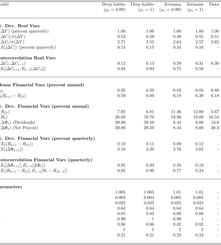
The results are summarized in Table 4. The bottom panel of the table summarizes the parameters used to simulate from each model. I generate 1000 simulations of 240 quarterly observations and report the average over all simulations. I consider both the case where productivity shocks are permanent (ρz = 1) and where productivity shocks are
highly persistent but transitory (ρz = 0.99). I calibrate the volatility of the productivity
shocks to match the volatility of quarterly output growth, which equals 1 percent.
The table shows that both models are well able to match the unconditional moments of the data, including the volatility of consumption growth, investment growth, the equity risk premium and the level of the riskfree rate. By increasing the persistence of the habit stock (ρ), which Jermann (1998) sets equal to zero, the model is close to matching the volatility of the riskfree rate as well. Whereas the volatility of dividends seems too low in Jermann’s model, the deep habits model generates too volatile dividends compared to the standard measure of per share dividends. However, recent work by Bansal and Yaron (2006) and Yogo and Larrain (2007) suggests that the total net payout of firms is in fact more volatile than per share dividends. In particular, Yogo and Larrain (2007) find that the volatility of net payout growth equals 38 percent per year, which is close to the volatility generated by the deep habits model.
The models’ success in explaining the unconditional moments of the financial variables is contrasted by their poor performance in matching the conditional moments of the data. Most importantly, the variation in the price-dividend ratio is almost entirely driven by variation in expected dividend growth rates and the riskfree interest rate and not by variation in expected excess returns. The unconditional standard deviation of quarterly expected excess returns is only 0.1 percent as opposed to a standard deviation of quarterly expected dividend growth rates of 3.1 percent. Given that the persistence of both variables is approximately equal, the variance decomposition of the price-dividend ratio is dominated by riskfree rate and expected dividend growth rate variation.21 The variation in expected returns can be substantially increased by including preference shocks, that is shocks to the habit formation process.22 However, even in this case the model still generates substantial variation in expected growth rates. This expected dividend growth rate variation is in contrast to the habit formation model in an endowment economy as proposed by Campbell and Cochrane (1999).
21Furthermore, the correlation between expected excess returns and expected dividend growth rates is low
(not reported), which seems in contrast with the data (see for example Binsbergen and Koijen (2007) and Lettau and Ludvigson (2005)).
Finally, and interestingly, it seems that even when productivity shocks follow a random walk, expected consumption growth is time-varying and persistent induced by the high capital adjustment costs and persistence in the habit formation process, which smoothes out the influence of the productivity shocks, even when these productivity shocks are independently and identically distributed (i.i.d.). The high capital adjustment costs are necessary to match the level of the risk premium. The high persistence of the habit process (0.85) helps to match the low volatility of the risk free rate. In a recent paper, Kaltenbrunner and Lochstoer (2007) argue that in a general equilibrium framework with Epstein-Zin preferences, highly persistent expected consumption growth rates, as proposed in Bansal and Yaron (2004), arise endogenously from the consumption smoothing behavior of consumers even when productivity shocks are i.i.d.. However, it seems that habit formation models with production and capital adjustment costs also produce such persistent expected consumption (and dividend) growth rates.23
5
Empirical Evidence
The deep habits model suggests (1) a positive relationship between the consumption surplus ratio and expected returns and a negative cross-sectional relationship between the product prices of firms and the expected return on their stock. I empirically investigate both these relationships by sorting firms into quintile portfolios based on past consumption surplus ratios and recent price increases and decreases. I use annual data on NAICS industry shipments and Second, I use monthly data from the Producer Price Index (PPI) Program. The PPI measures the average change over time in the selling prices received by domestic producers for their output.
A direct test of the model would be to rank firms based on the price elasticity of their demand curves. Unfortunately, these price-elasticities are unobservable. If the demand elasticity of firms is constant, the slope of the demand curve can be uncovered through an instrumental variables analysis involving exogenous shocks of the supply curve. However, in my model demand elasticities are time-varying as each good’s price elasticity of demand is proportional to the consumption surplus ratio of that good. Instead I will focus on these consumption surplus ratios and price changes within industries.
23Note that this suggests that in a production economy the question may not be so much whether expected
dividend and consumption growth rates are time-varying or not, but rather whether consumers care about such time variation in their preferences.
5.1
Data
The Bureau of Economic Analysis publishes annual data with quantity indexes on GDP for 423 industries between 1997 and 2008. Merging with the CRSP data based on NAICS code, this results in annual data between 2001 and 2008. I then use these quantity indexes to construct a habit level and a consumption surplus ratio.
The PPI tracks price changes for practically the entire output of domestic goods-producing sectors: agriculture, forestry, fisheries, mining, scrap, and manufacturing. Further, in recent years, the PPI has extended coverage to many of the non-goods producing sectors of the economy, including transportation, retail trade, insurance, real estate, health, legal, and professional services and new PPIs are gradually being introduced for the products of industries in the utilities, finance, business services, and construction sectors of the economy.24
The PPI sample I use includes over 25,000 establishments providing approximately 100,000 price quotations per month. Participating establishments report price data primarily through the mail. Goods and services included in the PPI are weighted by value-of-shipments data contained in the 1997 economic censuses. I use aggregated PPI data for industries based on the two digit Standard Industrial Classification (SIC) code between 1983 and 2003. After 2003, the PPI indexes based on SIC codes is discontinued and replaced by the North American Industry Classification System (NAICS). My choice of the SIC based PPI index as well as the data period and the level of SIC detail are motivated by the desire to maximize the compatibility between Center for Research in Security Prices (CRSP) and PPI data.
Merging CRSP data and PPI data based on the two-digit SIC codes results in monthly observations between 1983 and 2003 for 35 different industries. I then sort firms into five portfolios based on the percentage change of their PPI in the previous month. Quintile 1 contains firms whose PPI change was the lowest in the previous month, that is, who have the largest price decrease. Quintile 5 contains firms whose PPI change was the highest. I then compute value-weighted returns within each of these quintiles. I will refer to the portfolio that goes long in quintile portfolio 1 (Deflationary) and short in quintile portfolio 5 (Inflationary), as the DMI (Deflationary Minus Inflationary) portfolio.
5.2
Results
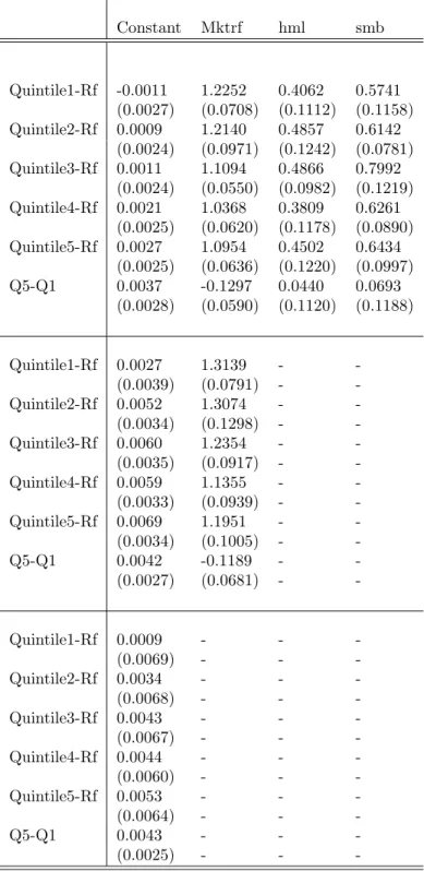
The first panel of Table 5 reports the results from the time series regressions of the excess returns of the quintile portfolios sorted on the lagged consumption surplus ratio between
2001 and 2008. The table also reports the regression of the Q5-Q1 portfolio on a constant term and the three Fama French factors. The factors, which I acquire from Kenneth French’s website, include the excess return on the market (mktrf), the book-to-market portfolio (hml), the size portfolio (smb). The Newey and West (1987) adjusted standard errors are reported in brackets. The results show that there is a upward monotonic pattern of the pricing error (or alpha) as the quintiles increase, with an alpha of -0.11 percent for quintile 1 and a pricing error of 0.27 percent for quintile 5. For the Q5-Q1 portfolio, the alpha is 0.37% per month which is equivalent to an annual return spread of 4.4%. The loading on the market portfolio is negative and significant, but economically small. Further the loading on the book-to-market portfolio and size portfolio is insignificant. The same monotonic pattern of alphas, can be seen when regressing excess returns on the market portfolio or just a constant. The p-value for the constant term in the regression is 0.08 for raw returns, 0.12 when regressing returns on the market portfolio and 0.18 when regressing returns on the three factors. Given the very short data period, this increase in p-values should be expected, as should be the relatively low level of significance.
The first panel of Table 6 reports the results from the time series regressions of the net excess returns of each of the quintile portfolios sorted on lagged producer price changes. The table also reports the Q5-Q1 (or DMI) portfolio on a constant term and the four factors. In this case, there is a downward monotonic pattern of the pricing error (or alpha) as the quintiles increase, with an alpha of 0.37 percent for quintile 1 and a pricing error of -0.21 percent for quintile 5. However, from quintile 4 to quintile 5, there seems to be a slight, statistically insignificant, increase in the pricing error from -0.29 to -0.21 percent. The DMI portfolio earns a monthly alpha of 0.58 percent, with a t-statistic of 2.31, which is significant at the 5 percent level. Interestingly, the loading of the DMI portfolio on the book-to-market factor is negative and statistically significant. This negative loading increases the alpha compared to the CAPM benchmark which I report in panel 2 of Table 6. Even though the CAPM alpha of 0.40 percent is smaller than the four-factor alpha, it is still significant at the 10 percent level with a p-value of 0.075. Finally, panel 3 of Table 6 reports the average return on each of the quintiles as well as the standard deviation of the mean. The average monthly return on the DMI portfolio equals 0.54 percent, which with a standard deviation of 0.29 percent is statistically significant at the 10 percent level.
The results in Table 6 are generated by sorting on the producer price index change in the previous month. The producer price index in a given month is computed based on individual price quotes from firms for their products. As these price quotes are public information, one would expect that when a firm changes its price, this change is immediately reflected in its
within an industry, is not reported until the second week of the next month. To rule out that my results are driven by ex post sorting on price increases, I also sort firms based on price changes over a 4-month period starting in month t−5 and ending at t−2. The results are reported in Table 7. As before, there is a downward pattern of the alpha as the quintiles increase, with a monthly alpha of 0.47 percent for quintile 1 and an alpha of -0.08 percent for quintile 5. However, similar to Table 6, the pattern is slightly upward sloping for the last two quintiles. However this increase is not statistically significant. The DMI portfolio earns a monthly alpha of 0.54 percent, with a t-statistic of 2.01, which is significant at the 5 percent level. Again, the loading of the DMI portfolio on the book-to-market factor is negative. Finally, panel 3 of Table 7 reports the average return on each of the quintiles as well as the standard deviation of the mean. The average monthly return on the DMI portfolio equals 0.68 percent. Because the standard deviation is 0.27 percent, this is statistically significant at the 5 percent level.
6
Robustness Checks
6.1
Z-scores of the PPI
In the previous section I have sorted firms into quintile portfolios based on their recent percentage price changes. This sorting generates a statistically significant alpha with respect to both the unconditional CAPM and the four factor model. In this section I explore the possibility that these results are driven by relatively few sectors whose percentage product price change are either highly volatile or have a mean that differs substantially from the percentage changes of the aggregate producer price index. To address this issue, I sort firms not based on percentage price changes, but based on Z-scores. That is, I compute for each industry the average percentage price change over time and its standard deviation. I then compute the Z-score by demeaning each months industry price change and then divide this demeaned value by its corresponding standard deviation. I then sort stocks into quintile portfolios based on the previous month’s Z-score. I find that sorts based on this criterion deliver almost identical results to those reported in the previous section.
6.2
Industry competition
As I discussed before, my model also relates to the recent literature on the cross-section of expected returns and product market competition. Hou and Robinson (2006) show that US
4% higher than those of similar firms in the quintile of the most concentrated industries. The market power that Hou and Robinson (2006) consider is related to the price setting behavior that I study in this paper. However, in my model, low expected returns are not a unconditional characteristic of an industry or firm but are a consequence of the current low income and price elasticities of demand faced by a particular firm or industry, which are time-varying and proportional to the consumption surplus ratio. When I construct the quintile portfolios, I indeed find that firms (and industries) frequently rotate across quintiles, as discussed in the next subsection. In contrast, firm sorts based on each industry’s Herfindahl-Hirschman Index (HHI), as in Hou and Robinson (2006), can be used to generate a spread in expected returns up to several decades into the future. In Table 8 I include the return spread on the HHI portfolios as an addititional factor. The table shows that the DMI portfolio that I construct does not significantly load on the HHI factor and the generated alpha is still significant at the 5% significance level.
6.3
Markov matrices
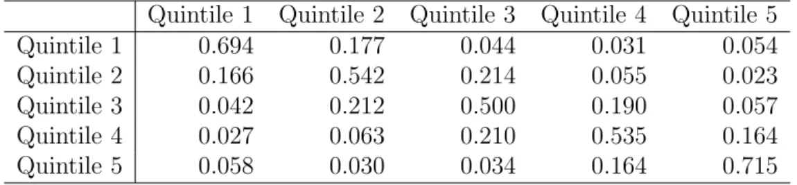
To confirm that firms and industries frequently rotate across the quintile, I compute in table 9 the quarterly Markov probabilities of each firm in my dataset. The (i,j) element represents the probability of a firm switching from quintile i to quintile j over a one quarter horizon. The matrix shows that even though there is persistence in the quintiles, there is substantial variation across industries. For example, when computing the 3-year Markov probabilities by taking the reported matrix to the power 12, it is easy to see that these probabilities are nearly equal to the unconditional probability distribution of 0.20 for each quintile.
7
Discussion and Extensions
In this paper I have argued that the deep habits model can help to explain part of the variation in the cross-section of expected returns. In particular, the model explains why there are expected return differences between firms with recent price decreases and recent price increases. However, so far the model has not addressed the question of why there is a value or a size premium. This question is particularly interesting in a habit formation context because recently Lettau and Wachter (2007) and Santos and Veronesi (2006) have raised the issue that growth firms have high duration cash flows and are therefore more susceptible to discount rate risk. Because in habit formation models the shocks to the consumption surplus ratio (which drives expected returns) and shocks to consumption growth are perfect correlated, growth firms should carry a premium relative to value firms. Lettau and Wachter (2007)
argue that to solve this problem, variation in the discount factor should be independent of cash flow shocks. They then model the variation in the discount factor in a reduced form setting and argue for a zero (or negative) correlation with cash flow growth shocks. As they assume that cash flow growth shocks are the only shocks that are priced, this allows for a zero or even negative risk premium on discount rate shocks.
Lettau and Wachter (2007) suggest that the discount rate variation could be due to a preference shocks, but it is not obvious why such preference shocks would carry a zero or negative price of risk. In contrast, the deep habits model endogenously generates a negative risk premium on preference shocks for those firms with a high habit level, because such firms can increase their prices the most in response to these systemic shocks. Furthermore, in the aggregate, the model generates a markup of prices over marginal costs which increases in response to a positive aggregate preference shock, again providing a (partial) hedge against systematic preference shocks. As such, the deep habits model seems a promising framework in which to study the value premium, which I will address in future research.
8
Conclusion
I study the cross-section of expected returns in a general equilibrium framework where instead of forming habits over some aggregate consumption bundle, agents form habits over individual varieties of goods. Goods are produced by monopolistically competitive firms, whose price-elasticity of demand depends on the habit formation for their specific good. As such, the model generates a strong relationship between the expected return on a firm’s stock and the selling price of its product, which are both driven by the firm’s habit stock. Firms with a high habit stock earn low expected returns and charge high prices for their product. I investigate this relationship empirically by sorting firms into five quintiles based on recent price changes, as measured by the producer price index. This sorting generates a statistically significant annual alpha of 6 percent that can not be explained by the four-factor model. I show that the CAPM seems to price the PPI portfolios better than the four-factor model, because firms with recent price decreases earn high expected returns, but load negatively on the book-to-market factor.
References
Abel, A. B. (1990): “Asset Prices Under Habit Formation and Catching Up With the Jones,”
American Economic Review, 80, 38–42.
Ait-Sahalia, Y., J. A. Parker, and M. Yogo (2004): “Luxury Goods and the Equity Premium,”Journal of Finance, 59(6), 2959–3004.
Bansal, R., and A. Yaron (2004): “Risks for the Long-Run: A Potential Resolution of Asset Pricing Puzzles,” Journal of Finance, 59(4), 1481–1509.
(2006): “The Asset Pricing-Macro Nexus and Return-Cash Flow Predictability,” Unpublished paper, Duke University.
Binsbergen, J. v., and R. Koijen(2007): “Predictive Regressions: A Present-Value Approach,” Unpublished paper, Duke University and NYU Stern.
Boldrin, M., L. J. Christiano, and J. D. M. Fisher (2001): “Habit Persistence, Asset Returns and the Business Cycle,”American Economic Review, 91(1), 149–166.
Campbell, J. Y., and J. H. Cochrane (1999): “By Force of Habit: A Consumption-Based Explanation of Aggregate Stock Market Behavior,”Journal of Political Economy, 107, 205–251. (2000): “Explaining the Poor Performance of Consumption-Based Asset Pricing Models,”
Journal of Finance, 55(6), 2863–2878.
Cochrane, J. H. (2006): “The Dog That Did Not Bark: A Defense of Return Predictability,”
Review of Financial Studies, forthcoming.
Constantinides, G. M.(1990): “Habit-formation: A Resolution of the Equity Premium Puzzle,”
Journal of Political Economy, 98, 519–543.
Cooper, R., and J. Haltiwanger(2000): “On the Nature of Capital Adjustment Costs,” NBER working paper 7925.
Cooper, R., and J. Willis(2004): “The Cost of Labor Adjustment: Inferences From the Gap,” Working paper Federal Reserve Bank of Kansas.
Dixit, A. K., and J. E. Stiglitz (1977): “Monopolistic Competition and Optimum Product Diversity,” American Economic Review, 67(3), 297–308.
Gala, V. (2006): “Investment and Returns,” PhD Dissertation, University of Chicago.
Gomes, J. F., L. Kogan, and M. Yogo (2006): “Durability of Output and Expected Stock Returns,” Wharton.
Guadagni, P., and J. D. Little(1983): “A Logit Model of Brand Choice Calibrated on Scanner Data,”Marketing Science, 2(3), 203–238.
Heaton, J. (1995): “An Empirical Investigation of Asset Pricing with Temporally Dependent Preference Specifications,” Econometrica, 63, 681–717.
Hou, K., and D. T. Robinson (2006): “