C
ONSUMPTION
I
NEQUALITY AND
I
NTRA
-H
OUSEHOLD
A
LLOCATIONS
Jeremy Lise
Shannon Seitz
Consumption Inequality and Intra-Household
Allocations
∗
Jeremy Lise
†University College London
and Institute for Fiscal Studies
Shannon Seitz
‡Boston College
and Queen’s University
July 4, 2007
Abstract
The consumption literature uses adult equivalence scales to measure individual level in-equality. This practice imposes the assumption that there is no within household inin-equality. In this paper, we show that ignoring consumption inequality within households produces mis-leading estimates of inequality along two dimensions. First, the use of adult equivalence scales
underestimates the level of cross sectional consumption inequality by30%, as large differences
in the earnings of husbands and wives translate into large differences in consumption alloca-tions within households. Second, the rise in inequality since the 1970s is overstated by almost two-thirds: within household inequality declined over time as the share of income provided by wives increased. Our findings also indicate that increases in marital sorting on wages and hours worked can simultaneously explain virtually all of the decline in within household in-equality and a substantial fraction of the rise in between household inin-equality for one and two adult households in the UK since the 1970s.
JEL Classification: D12, D13, D63, J12, J22
Keywords: Collective Model, Consumption Inequality, Marital Sorting, Adult Equivalence Scales
∗We would like to thank Garry Barrett, Richard Blundell, Martin Browning, Chris Ferrall, Bernard Fortin, Allen
Head, Bev Lapham, Arthur Lewbel, Frank Lewis, Hao Li, Huw Lloyd-Ellis, Mary MacKinnon, Costas Meghir, Kr-ishna Pendakur, José-Víctor Ríos-Rull, the editor, three anonymous referees and participants at numerous conferences and seminars for many helpful comments.
†[email protected]. Department of Economics, University College London, Gower Street, London, WC1E 6BT ‡[email protected]. Department of Economics, Boston College, Chestnut Hill, MA, 02467
1 Introduction
A recent literature has documented a large rise in consumption inequality in several developed countries.1 Underlying these measures of inequality is the use of adult equivalence scales, which are used to assign consumption levels to each member of a household. This has been necessary as there do not exist comprehensive measures of individual level consumption for households with more than one member. The drawback of this approach is that it implicitly assumes there is no inequality among adults within the household. In particular, the use of adult equivalence scales implies a very restrictive model of the household in which husbands and wives split consumption equally, regardless of the source of the income.2
This equal division assumption is inappropriate in the study of consumption inequality, as a large theoretical and empirical literature routinely rejects the assumption that the consumption allocation does not vary with the source of income in the household (Browning, Bourguignon, Chiappori and Lechene, 1994; Browning and Chiappori, 1998; Chiappori 1988, 1992; Chiappori, Fortin and Lacroix, 2002; Donni, 2007; Lundberg, Pollak and Wales, 1997; Manser and Brown 1980; McElroy and Horney, 1981, among many others). Since there has been a sizable increase in women’s wages and labour supply over the last half century, the share of household earnings provided by the wife has changed substantially over time. If consumption allocations depend on the source of income and the sources of income within households have changed over time, then adult equivalence scales will produce an inaccurate picture of the trends in consumption inequality. The goal of this paper is to document the trends in consumption inequality once within house-hold inequality is taken into account. We construct and estimate a static model of intra-househouse-hold allocations to examine how changes in the source of income in the household translate into changes
1See Blundell and Preston (1998) for the UK, Pendakur (1998) for Canada and Barrett, Crossley and Worswick
(2000) for Australia. The evidence on consumption inequality in the United States is mixed. Slesnick (2001) and Krueger and Perri (2006) do not find a large rise in consumption inequality since the 1970s. Alternatively, Cutler and Katz (1992) and Johnson and Shipp (1997) report a rise in inequality. Attanasio, Battistin and Ichimura (2007) use two sources of data on consumption and also find consumption inequality was rising over time.
2Recently, there has been a substantial departure from this literature. Browning, Chiappori and Lewbel (2006)
relax the assumption that household members split consumption equally in the construction of adult equivalence scales. Hong and Ríos-Rull (2007) use information on the purchase of life insurance to estimate equivalence scales.
in individual-level consumption allocations. In particular, we observe variation in labour supply, total household consumption and wages for singles and married couples in the data. We use the joint relationships between consumption, wages and labour supply for single households and be-tween own and spousal wages in married households to infer the private consumption levels for married men and women. The model is estimated on a sample of one and two person households from the UK Family Expenditure Survey (FES) for the years 1968 to 2001. Under relatively weak identification assumptions, the model allows us to infer the level of consumption allocated to each member of the household, which is necessary for the measurement of individual level consumption inequality.
We then use our estimates to construct a new measure of consumption inequality across indi-viduals. We have two main findings. First, ignoring the potential for intra-household inequality may underestimate individual-level consumption inequality by 30%, as differences in earnings across husbands and wives generates substantial within-household inequality. Second, the rise in consumption inequality reported in the literature is overstated by almost two-thirds. This result is due to the fact that within household inequality has fallen over time as female wages and labour supply have increased. An implication of our findings is that the equal sharing assumption implicit in adult equivalence scales is validonlyfor households in which the wife has the same earnings as her husband.
A recent literature examines several dimensions of the relationship between inequality and household behavior. Kremer (1997) and Fernández and Rogerson (2001) consider the extent to which increases in marital sorting cause increases in inequality. Fernández, Guner and Knowles (2005) and Dahan and Gaviria (1999) present empirical evidence of a positive correlation between sorting and inequality.3 Gould and Paserman (2003) consider whether male wage inequality has a causal effect on marriage and find that increases in inequality lead to reductions in marriage rates. We contribute to this literature by providing evidence on the importance of several potential
3In this instance, the degree of marital sorting is measured by the correlation between characteristics such as
explanations for the rise in consumption inequality between households and the fall in inequality within households since the 1970s in the UK. While changes in the demographic composition of the population appear to play a limited role, an increase in marital sorting has profound effects on the trends in consumption inequality. In particular, the rise in marital sorting on wages and hours observed in the data has the potential to account for all of the fall in within household inequality and at the same time can explain a large fraction of the rise in consumption inequality between households.
The remainder of the paper is organized as follows. Section 2 describes in detail the stylized facts on consumption, wages and labour supply that provide the motivation for our study. Section 3 outlines the theoretical framework and the identification strategy for estimating the rule to allocate consumption to individuals within a household. Section 4 describes the data set and Section 5 the strategy for estimating the model. The estimation results are presented in Section 6. Sec-tion 7 presents a decomposiSec-tion of consumpSec-tion inequality and considers the importance of several explanations for the trends in consumption inequality. Section 8 concludes.
2 Trends in Consumption and Earnings Inequality in the UK
In this section, we outline the main stylized facts regarding consumption and income inequality in the UK between 1968 and 2001. The data we use to conduct our analysis comes from the UK Family Expenditure Survey (FES). The FES contains information on household consumption ex-penditures and earnings over the period 1968 to the present. In the construction of the following stylized facts, we restrict the sample to individuals between the ages of 16 and 65 and eliminate stu-dents, retirees and the self-employed. We are particularly interested in the following four features of the data:
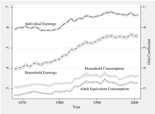
1. There has been a large rise in earnings inequality between individuals. Figure 1 documents the trend in the Gini index for the distribution of individual and household earnings. The Gini index for individual earnings has risen by 12% over the past 30 years. This rise in
earnings inequality in the UK has been well documented in the literature (e.g. Blundell and Preston, 1998).
2. Although earnings inequality between individuals is much higher than earnings inequality between households, the latter rose much more rapidly: the Gini index for inequality between households rose by41%between 1968 and 2001.
3. As reported by Blundell and Preston (1998), there has been a corresponding rise in con-sumption inequality. To account for economies of scale, we construct a standard measure of individual-level consumption by dividing total household consumption by the square root of household size. The Gini index for this measure of consumption is presented Figure 1. The level of earnings inequality is higher than the level of consumption inequality but the rise in inequality is higher for consumption than for earnings.
4. As illustrated in Figure 2, the correlation between the earnings of husbands and wives in-creased dramatically over time. At the same time, the gender wage gap dein-creased and female labour supply increased. Figure 3 highlights the dramatic change in the gender wage gap and in women’s contribution to household labour income between 1968 and the present. The dashed line represents the female’s share of potential income, defined as the share of labour earnings that would be contributed by the wife if both spouses worked full-time.4 The solid line represents women’s share of actual household earnings. Overall, potential earnings of wives increased by 13.5%, and women’s share of earnings in the household increased by 93%over the sample period. The latter partly reflects the increase in women’s wages rela-tive to those of men, but also the large changes in female and male employment rates and hours worked since the 1960s.
In summary, the evidence presented here highlights the fact that there has been a large rise in earnings and consumption inequalitybetweenhouseholds while at the same time there has been a
4For households with missing wage data due to non-participation, we include a predicted wage based on a standard
fall in inequality in the earnings distributionwithinhouseholds.
3 Model
In this section, we present a model that allows us to infer the level of consumption for each member of a household. The model is based on Chiappori’s (1988, 1992) collective model of household decision making.5 This framework is less restrictive than the model of equal division underlying adult equivalence scales, as the only restriction on the intra-household allocation process is that households reach Pareto efficient allocations.
We modify the basic collective model along three dimensions to address several issues of rele-vance to our analysis. First, to account for the lumpiness of labour supply observed in the data, we allow individuals to choose zero, part-time or full-time hours of work.6 Second, we make a distinc-tion between private and public consumpdistinc-tion in the model. As public consumpdistinc-tion is consumed by both members of the household, ignoring the presence of public consumption may overestimate the degree of inequality within households. We follow the strategy of Browning et al. (1994) and partition all expenditures into either public or private expenditures. The goal of the estimation exercise is to determine the allocation of private expenditures across household members.
Third, as in Vermeulen (2004) and Browning, Chiappori and Lewbel (2006), we need to impose additional restrictions on the collective model to identify the entire sharing rule. The question we aim to address in this paper is whether measures of consumption inequality from the collective model differ from measures in the literature based on standard equivalence scales. To answer this question, we require an estimate of the full sharing rule to uncover the share of income allocated to each household member for consumption. We assume that the sub-utility over private consumption
5See also Browning et al. (1994), Browning and Chiappori (1998), Chiappori et al. (2002) and Blundell et al.
(2007).
6Blundell et al. (2007) model the labour force decision of the wife as continuous and of the husband as discrete;
either he works full-time or not at all. Donni (2003) considers the labour force participation decision and Vermeulen (2004) considers the case where males are assumed to work full-time and females face a discrete labour supply choice which includes the option of non-participation. As in our application, Vermeulen et al. (2006) treat the labour supply decisions of both spouses as discrete.
and leisure is the same when married as when single. In Section 6, we test whether this assumption is supported by the data.
We start with a general description of the problem faced by single agents. We then describe the intra-household allocation decision of married couples and the model restrictions that allow for the identification of the share of private consumption allocated to each household member.7
3.1 Singles
Assume all single individuals have preferences over leisure and consumption. For individuals of genderg, denote discrete labour supply choices hg, hg ∈ H, leisure Lg, expenditures on private consumptionCg, and expenditures on public consumption Pg. The total time available isT, i.e.
hg =T −Lg.
Assume preferences for public consumption are separable from preferences over private con-sumption and leisure. Denote total household non-labour income net of savings byYg. After tax labour earnings are denoted wg(hg), where the notation is chosen to reflect the progressive na-ture of the tax system. Labour earnings includes all after tax income that depends directly on the labour supply decision. In particular, wg(hg) includes unemployment insurance benefits paid to individuals who are not working. Single agents maximize utility by choosing labour supply and the allocation between public and private consumption goods
max Cg,Pg,LgU
g(ug(Cg, Lg), Pg) subject to
Cg+Pg =wg(hg) +Yg, hg+Lg =T, andhg ∈H.
Using the separability assumption, we appeal to two-stage budgeting in which the individual first chooses the level of public goods expenditure and in the second stage faces the problem
max Cg,Lgu
g(Cg, Lg) (1)
7Of course there are many aspects of the household’s problem that we do not address, including savings and risk
subject to the second stage budget constraint
Cg =wg(hg) +yg,
whereyg =Yg −Pg,hg+Lg =T, andhg ∈H.
3.2 Married Couples
Consider a two member household, where each member has distinct preferences over own leisure, own private consumption, and household public consumption. As with singles, we assume that preferences over private consumption and leisure are separable from consumption of the public good. Since public consumption is assumed to be consumed by both household members (Pf =
Pm = P), it is only necessary to uncover the sub-utility for private consumption and leisure and the sharing rule to determine the share of consumption allocated to each household member. Preferences over public consumption, which we do not estimate, are allowed to vary freely with marital status.
Under the assumptions that preferences are egoistic and that allocations are Pareto efficient, the household’s allocation can be represented as the solution to the problem:
max
Cf,Cm,Lf,Lm,PλV
f ¡vf(Cf, Lf), P¢+ (1−λ)Vm(vm(Cm, Lm), P),
subject to
Cf +Cm+P =wf(hf, hm) +wm(hm, hf) +Y, hg+Lg =T, andhg ∈H.
where the Pareto weight,λ, represents the female’s relative bargaining power within the household. The notation wf(hf, hm)accommodates the fact that, prior to 1990, the tax system in the UK is progressive and based on household as opposed to individual incomes. As a result, after-tax wages and non-labour incomes depend on the labour supply decisions of both spouses.
In the case without joint taxation, Blundell, Chiappori and Meghir (2005) show that the intra-household allocation problem faced by a husband and wife can be decentralized by considering
a two stage process. In the first stage the husband and wife decide on the level of public good consumption (P) and on how to divide the remaining non labour income y = Y −P. The as-sumption that utility from leisure and private conas-sumption are separable from conas-sumption of the public good is key to allowing the allocation of public consumption to occur in the first stage. The joint taxation of incomes complicates the decentralization of the household problem.8 To address this complication we define the conditionalearnings for individuals of gender g, ωg(hg, hg0
∗), as the after tax earnings of an individual workinghg hours conditional on the actual labour supply of spouseg0,hg0
∗.
The household’s problem can then be decentralized as follows. In the first stage, households agree on an efficient level of public goods expenditures and a sharing rule to divide the remaining non-labour income. Define the sharing rule φ(y,ω¯f,ω¯m, z)as the amount of non-labour income that is assigned to the wife. The sharing rule is assumed to depend on conditional earnings for the wife and husband, ω¯f and ω¯m respectively, when both partners work full-time (40 hours per week).9 The distribution factor,z, is a factor that influences the Pareto weight but does not directly affect preferences. In the second stage, each household member chooses labour supply and private consumption to maximize utility. The problem facing the wife in the second stage is:
max Cf,Lfv
f(Cf, Lf) (2)
subject to
Cf =ωf(hf, hm∗ ) +φ(y,ω¯f,ω¯m, z), Lf +hf =T, hf ∈H,
and the husband faces the problem
max Cm,Lmv
m(Cm, Lm) (3)
subject to
Cm =ωm(hm, hf∗) +y−φ(y,ω¯f,ω¯m, z), Lm+hm =T, hm ∈H.
8We thank a referee for pointing out this issue. With few exceptions, e.g. Donni (2003) and Vermeulen (2006), the
literature on collective models ignores taxation.
9The reason the sharing rule is assumed to depend on potential earnings, as opposed to actual earnings, is that the
3.3 Identification
Before discussing identification, we select functional forms for preferences and the sharing rule. We specify a CES sub-utility function
ug(Cg, Lg) = £αg(Cg)ρg
+ (1−αg)(Lg)ρg¤1/ρg
and a linear sharing rule:
φ(y,ω¯f,ω¯m, z) = · φ0+φ1 ¯ ωf ¯ ωf + ¯ωm +φ2 ³ Agem−Agef´¸y,
where the spousal age gap is introduced as a distribution factor. Wages enter the sharing rule here as the female’s potential share of conditional earnings, when both spouses work full-time, to capture the notion that relative earnings power is likely to influence the intrahousehold allocation of resources.
As mentioned above, our primary interest is in allocating private consumption between the household members. This requires that we obtain an estimate of the sharing ruleφ(y,ω¯f,ω¯m, z). Generically, this sharing rule is identified up to a constant (Chiappori; 1988, 1992). Our exercise requires complete identification of the sharing rule which requires an additional restriction. As in Browning, Chiappori, and Lewbel (2006) among others, we assume that some features of pref-erences do not change following marriage. In particular, we assume the sub-utilities over private consumption and leisure do not change following marriage: vg(C, L) = ug(C, L). The prefer-ence parameters αg and ρg can then be identified using data on singles, if labour supply, wages, and non-labour incomes for singles are observed. Given identification of sub-utilities, the sharing rule is identified as the share of household non-labour income that rationalizes the observed labour supply choices of married men and women.
4 Data
The data we use comes from the UK Family Expenditure Survey (FES). This data is ideal for the study of consumption inequality for three reasons. First, it contains detailed information on private
and public consumption expenditures for households, on wages and labour supply for individuals, and on demographics including age, education (from 1978 onward) and region of residence. Sec-ond, the FES has fewer problems with measurement issues than the leading contenders in the US and elsewhere.10 The FES uses a weekly diary to collect data on frequently purchased items and uses recall questions to collect data on large and infrequent expenditures. Finally, the FES contains information over the period 1968 to the present, which allows the study of changes in consumption inequality over a long period of time.
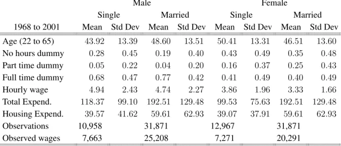
Our sample contains single person households and couples without children.11 We restrict the age range in the sample to individuals between the ages of 22 and 65 and eliminate students and the self-employed. For robustness, households in which one of the individuals is in the top one per cent of the wage distribution are also excluded. The resulting sample contains 87,668 individuals.12 Descriptive statistics for our entire sample are presented in Table 1.
We define consumption and non-labour income measures as follows. Total consumption is de-fined as total household expenditures. Public consumption is dede-fined as expenditures on housing, light and power, and household durable goods. Private household consumption is total expendi-tures net of public consumption. Other income is defined as total household expendiexpendi-tures minus net labour income. We use this expenditure based definition of non-labour income, as it is con-sistent with the assumptions of a two stage budgeting process, time separable preferences, and separability of public goods consumption from leisure and private consumption as in the model.13
To construct the level of consumption corresponding to each labour supply decision, including zero hours, we need to assign an earnings level to all individuals. For those who are working we
10Battistin (2004) documents reporting errors in the US Consumer Expenditure Survey due to survey design. 11We exclude households with children in this paper to abstract from the intra-household allocation of resources
for children’s consumption. This is obviously an important issue. To this end, our estimates of the sharing rule and the comparison of various inequality measures only apply to households without children. We leave to future work an analysis of consumption inequality for the entire sample of households.
12The sample size in 1968 is 2,584 and the sample size in 2001 is 2,757. The sample sizes do not vary markedly
across years: the smallest sample is 2,502 in 1979 and the largest is 2,932 in 2000.
13In estimation, household expenditures on public goods are subtracted from other income, resulting in non-labour
income net of public goods consumption. In addition to the separability assumptions, wage profiles are assumed to be exogenous. This rules out the possibility of job-specific human capital accumulation.
use the usual hourly wage, defined as weekly earnings divided by usual weekly hours. For non-participants we use a predicted wage, computed based on a reduced form selection-corrected wage equation. The log of the wage is estimated as a function of age, birth cohort, year, quarter and regional dummies, plus the age at which full time education was completed and its square. The selection equation is identified by the exclusion from the wage equation of household non-labour income, marital status, and the age, education and the labour income of the spouse.14 After tax earnings are subsequently computed by converting weekly wage income to an annual base, de-ducting the appropriate personal allowance and then applying the appropriate tax rate. Personal allowances and marginal tax rates are from the Board of Inland Revenue (1968–2001). All mone-tary values are expressed in 1987 pounds. The resulting income measure is treated as known and is used to construct thepotentialshare of after-tax household labour income contributed by the wife, ¯
ωf/(¯ωf + ¯ωm). Individuals may also be entitled to income related to earnings when working zero hours, for instance unemployment benefits, so we also predict unemployment benefits for those who are working based on theOfficial Yearbook of the United Kingdom (1968-2001).
Labour supply is measured by a discrete variable that takes on three values: not participating, working part-time and working full-time. Full time is defined as working 35 hours per week or more, and part-time is defined as 1 to 34 hours per week. The choice of these ranges is based on the hours histograms in Figure 4, which suggests a full-time definition of 35 hours a week or more. The average hours worked in the part-time category is approximately 20 hours per week, and approximately 40 hours per week in the full-time category.
In order to ensure consistency between the number of hours worked in each of the three states and the corresponding consumption level we adopt the following convention. If an individual is observed to be working either part-time or full-time we use the reported number of hours to measure labour supply and usual take home pay in constructing consumption. In cases for which we do not observe the labour supply state, we calculate after tax earnings based on 20 hours for the part-time choice and 40 hours for the full-time choice. Constructing individual consumption in this
way ensures our measure of total consumption in the household is consistent with that observed in the data.
5 Econometric Specification
We make the following additions to the model before estimation. First, we introduce several sources of individual specific heterogeneity. We allow the weighting of private consumption rela-tive to leisure to differ across individuals according to a set of demographic characteristics includ-ing a quadratic in age, education and dummy variables for decade of birth:
αg(X i) =
exp(Xiγ) 1 + exp(Xiγ)
We also introduce additive unobserved individual heterogeneity in preferencesηih, specific to in-dividualiand labour supply choiceh
ηihg =νiLih+εih
which has two components. The first component is a normally distributed, individual-specific component which allows preferences over leisure to be correlated across labour supply choices, and possibly with non-labour income (discussed below). The second component is i.i.d. type I extreme value preference heterogeneity.
Second, we treat labour income as endogenous and measured with error. Much of non-labour income depends on past non-labour income and thus may be endogenous to current non-labour supply decisions. To control for this potential endogeneity, we instrument nonlabour income using capital gains in the local housing market (as in Hurst and Lusardi, 2004), a cubic in reported asset income with time varying coefficients, an indicator for positive net worth, a quadratic in age for both part-ners, education for both partners and birth cohort dummies as instruments.15 Capital gains in the housing market are measured by quarterly year-over-year changes in real house prices in each of 12 regions in the UK, interacted with a home ownership indicator. The estimating equation for
nonlabour income for householdiis
Yi =Wiβ+²i (4) whereWi is the above set of instruments. Predicted non-labour incomeYˆi =Wiβˆis used in place of Yi and unobserved preferences for leisure, through νi, are allowed to be correlated with the residual²i. Finally, we set the total time endowment toT = 112hours per week or16hours per day.
Making use of these functional forms, along with the budget and time constraints, we can write the value of labour supply choiceh∈Hfor a single individual as
Vhg(Z, θ) = (αg(X) [wg(hg) +y]ρg + (1−αg(X)) [T −hg]ρg)1/ρg +νgLg h+εgh, and for a married woman and man as
Vhf(Z, θ) = ³ αf(X) · ωf(hf, hm ∗ ) + µ φ0+φ1 ¯ ωf ¯ ωf + ¯ωm +φ2(Age m−Agef) ¶ y ¸ρf + (1−αf)£T −hf¤ρf ´1/ρf +νfLf h +εfh, Vm h (Z, θ) = ³ αm(X) · ωm(hm, hf ∗) +y− µ φ0+φ1 ¯ ωf ¯ ωf + ¯ωm +φ2(Age m−Agef) ¶ y ¸ρm + (1−αm(X))[T −hm]ρm ´1/ρm +νmLm h +εmh,
where Z contains all relevant observables relating to both the individual and the choice and θ
contains all preference parameters and sharing rule parameters to be estimated.
Estimation proceeds in the following steps. First, we estimate a selection-corrected wage equa-tion and predict wages for individuals that are not working, as described in Secequa-tion 4. Second, we estimate the reduced form equation for non-labour income to obtain the predicted non-labour in-come Yˆ and the residuals. Third, we obtain estimates of the preference parameters αg, ρg, and
σg
ν by estimating a mixed multinomial logit model for the discrete labour supply choice using the subsample of single men and women. Lastly, we obtain estimates of the sharing rule parametersφ
men and women (conditional onαˆg,ρˆg, andσˆg
ν).16 The reported standard errors are bootstrapped to account for the multistage estimation procedure.
6 Estimation Results
We begin with estimates of the preference parameters, presented in Table 2. At the parameter estimates the utility function is increasing and quasi-concave for all the data. The elasticity of substitution ( 1
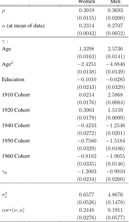
1−ρ) indicates the degree of substitutability between private consumption and leisure is similar across gender, 1.64for women and1.58for men. The share parameters are also quite similar for women (0.2314) and men (0.2707) at the mean, with a larger share going to leisure than private consumption, although the share parameter for males tends to vary across type to a greater extent than for females. Males also display substantially more variation in unobserved preferences over leisure, as indicated by the variance ofν. Finally, the results suggest that unobserved prefer-ences for leisure are positively correlated, and to the same degree, with the unobserved component of nonlabour income for both men and women.
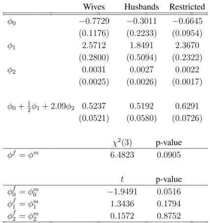
We now turn to the estimates of the sharing rule parameters, the parameters that allow us to infer the share of consumption attributed to each adult in the household. As discussed in Section 3, under the assumption that the sub-utility over private consumption and leisure is the same for mar-ried and single individuals, we can construct each of the sharing rule parameters independently from the labour supply decisions of the wife and the husband. The sharing rule parameters re-covered separately from the wife’s and husband’s labour supply decision are presented in the first and second columns of Table 3, respectively. The estimated sharing rule parameters constructed
16The contribution of an individualito the likelihood function is the probability of observing individualimaking
labour force decisionh, which has the mixed multinomial logit form (McFadden and Train, 2000):
L(h, Zi, θ) = Z 1 PH j=0exp(V g j(Zi, θ)−Vhg(Zi, θ)) dF(ν|²).
We partitionθinto the set of preference parameters,θ0 ={α, ρ, σν}and the set of sharing rule parametersθ1=φ.
Thenθˆ0= arg max P
i∈S`i(h, Zi, θ0), andθˆ1= arg max P
i∈M`i(h, Zi, θ1|θˆ0), whereSandM are the subsets of
separately from the wife’s and husbands estimates are qualitatively and quantitatively similar. In both specifications, the positive sign on φ1 indicates that an increase in the female’s share of
po-tential earnings increases her share of net nonlabour income in the household. The estimates also indicate that the spousal age gap has an economically and statistically insignificant effect on the intra-household allocation.
The test statistics associated with several tests of the model predictions are presented in the bottom four rows of Table 3. A Wald test on the full set of restrictions from the model does not reject the model at the 5 percent significance level, but does reject at the 10 percent level. We also test whether each of the individual restrictions from the female’s problem are consistent with the corresponding restrictions from the male’s problem. The test statistics indicate that none of the model restrictions are rejected at the5percent level and that the restrictions onφ1 andφ2 are
not rejected at any conventional significance levels. The marginal p-value for the restriction on the intercept in the sharing rule may be evidence of an intercept shift in preferences following marriage; unfortunately, it is not possible to separately identify such a shift in preferences and the intercept of the sharing rule in our specification. Overall, the test statistics provide some support for our version of the collective model.
We next estimate a version of the model that imposes the across-spouse restrictions on the sharing rule. The results of this exercise are presented in column three of Table 3. The estimates suggest that a10percent increase in the share of potential earnings attributed to the wife results in a24percent increase in the share of non-labour income she receives. This result is consistent with an increase in the wife’s threat point within a bargaining model.
6.1 Adult Equivalence Scales Revisited
One of the main goals of this paper is to determine whether measures of consumption inequality using standard adult equivalence scales provide an accurate estimate of consumption inequality across individuals. Recall, adult equivalence scales assume that husbands and wives share in household consumption equally. In this section, we determine the conditions under which our
model would yield the same measures of consumption inequality as measures using adult equiva-lence scales. We set the age difference between spouses to the average age difference in the data. We then use the sharing rule estimates to determine what value of the female’s share in potential household earnings satisfies:
1 2 = ˆφ0 + ˆφ1· ¯ ωf ¯ ωf + ¯ωm + ˆφ2·(2.09).
Using estimates forφ0,φ1andφ2of−0.6645,2.3670and0.0022, respectively, yields49%. In other
words, the model predicts that consumption is split equally across the husband and wife when they have the same earnings!17 It is worth emphasizing that this result is derived not from a model in which equal sharing is assumed: the only assumptions imposed in estimation are that households make Pareto efficient decisions, that public consumption is separable from private consumption, and that the marginal rate of substitution between leisure and private consumption is the same when single as when married.
6.2 Sensitivity Analysis
In this section, we consider the sensitivity of our results to both the sample used to estimate the model and the robustness of our estimation results to several modifications. First, we consider whether the trend in inequality measured in the literature for the entire population differs from the trend for our sample of one- and two-person households. Upon examination of Figure 5, we see that the trends in between household inequality using adult equivalence scales are virtually the same across samples. Thus, it does not appear that our results are driven exclusively by trends in inequality that are unique to our sample. That said, we are not able to say how the trends in within household consumption inequality vary between our sample and the entire population without estimating an extended version of our model.
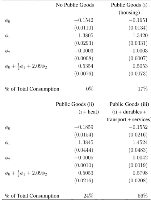
With regards to the robustness of our results, the first check we consider is whether the results are sensitive to our definitions of public and private consumption. We first estimate the model
17To be precise, husbands and wives will split consumption equally when they have approximately the same wages
under the assumption that there are no public goods and then sequentially add housing, heat and lighting, household durables, transport and services to public good consumption.18 The results of this exercise are reported in Table 4. The parameter estimates are quite robust across specifications: an increase in the wife’s share of potential household earnings of 10% results in an increase in her consumption share of between 14% and 15% and women receive between 51% and 58% of consumption in households where both spouses choose the same hours of work and have the same wage.
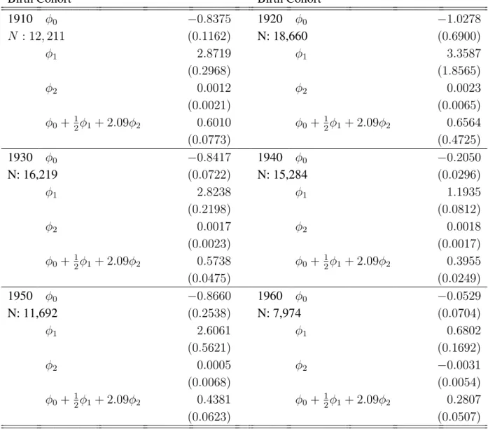
The next specification we estimate allows for differences in the sharing rule parameters for each birth cohort in our pooled sample. The sample covers a long time period and a wide age range in every year; we thus estimate sharing rules for each ten-year cohort in the data. The parameter estimates are presented in Table 5. There is some variability in the parameter estimates across cohorts, but no clear trend across time. For the cohorts between 1910 and 1960, an increase in the wife’s share of potential household earnings increases her share of non-labour income between 7% and34% and the estimated effect of an increase in the husband’s age by one year fall within the range of −0.3% and0.2%. With the exception of 1960, the share received by women when the husband and wife have the same earning potential is between 40% and60%, with the share received by women tending to decline for more recent cohorts.
7 Consumption Inequality
In this section, we compare the inequality measure implied by our model to a conventional mea-sure of consumption inequality. We use this sharing rule to divide non-labour income between the husband and wife in each household. We subsequently construct private consumption based on the individual’s share of non-labour income and his or her personal net labour earnings from each individual’s private budget constraint. Oursharing rulemeasure of individual consumption, for married individuals, is then equal to individual private consumption plus household public
18Estimating the full model with unobserved heterogeneity is computationally demanding. For this reason the
results pertaining to the sensitivity to the definition of public goods are obtained assuming a degenerate distribution for unobserved heterogeneity. Full estimation results are available from the authors upon request.
consumption: Cf =ωf(hf, hm∗ ) + · ˆ φ0+ ˆφ1 ¯ ωf ¯ ωf + ¯ωm + ˆφ2(Agem−Agef) ¸ y+P and Cm =ωm(h m, hf∗) + · 1−φˆ0−φˆ1 ¯ ωf ¯ ωf + ¯ωm −φˆ2(Agem−Agef) ¸ y+P.
Single individuals consume their entire labour and non-labour income. For comparison purposes, we construct another measure of individual consumption, equal division, which assumes that all consumption is divided equally between the husband and wife. In the equal division case, in-dividual consumption is calculated as household public consumption plus one half of household private consumption. In both thesharing ruleand theequal divisioncase, we double count public consumption. This accomplishes the same end as using an equivalence scale to assign household consumption to individual members.19
Having constructed these two measures of individual consumption, we can construct a time series of inequality measures and decompose them into changes in between and within household inequality. While the Gini coefficient is a well known and widely used inequality index, it does not allow overall inequality to be exactly decomposed into within and between group contributions. As this is one of the main objectives of this paper we also compute the Mean Logarithmic Deviation (MLD)20in consumption, defined as I(C) = 1 n n X i=1 log µ µC Cig ¶ , (5)
whereµC is the mean level of consumption. The index of total inequality using the MLD can be additively decomposed into within and between household inequality:
IT(C) =IW(C) +IB(C), (6)
19It should be noted that the correlation between our equal division consumption inequality measure and a measure
of inequality using equivalence scales is 0.99.
20The MLD is a member of the Generalized Entropy Class, the only class of additively decomposable inequality
whereIW(C)is within household inequality and IB(C)is between household inequality. Under the assumption of equal division, within household inequality is zero; therefore, we can calculate
IB(C)by using equal division. Using individual consumption constructed with the sharing rule we obtain the total inequality indexIT(C). We can then recover intra-household inequality using Equation (6).
7.1 Between and Within Household Consumption Inequality
The time-series trend of total and between household inequality for the years 1968 to 2001 is presented in Figure 6. The Gini index measures are presented in the first panel and the MLD mea-sures of inequality are presented in the second panel. Inequality was stable from 1968 to 1980 at which time it increased substantially until around 1990 and has been falling slightly from 1990 through 2001. The compression of marginal tax rates appears to have played a role in generating the sharp rise in between-household inequality during the 1980s. The top and bottom marginal tax rates are plotted in Figure 7, where the top marginal rate falls from 83% in 1978 to 60% in 1979, and then falls again to 40% in 1988. The increase in between household consumption inequality is closely linked to the increase in after tax income inequality that occurred over the 1980s. Of particular interest are two findings. First, ignoring intra-household inequality underestimates con-sumption inequality in 1968 substantially. This is due to the large differences in earnings between husbands and wives in 1968, differences that translate into an unequal distribution of consumption in the household. It is not surprising that our measure of inequality in 1968 is higher than the conventional measure: by definition, taking within household inequality into account will increase total inequality. However, the magnitude of the difference is striking: consumption inequality, as measured using adult equivalence scales, is underestimated by approximately 30% (15%) when inequality is measured using the MLD (Gini index). To put this figure into perspective, the dif-ference between the level of inequality in 1968 using our measure of inequality compared to the conventional measure is as large as the entire increase in inequality between 1968 and 2001.
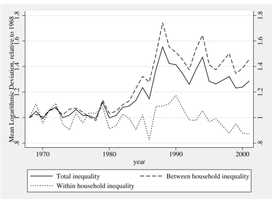
inequal-ity, may be over-stated by almost two-thirds, as illustrated by the trend in the MLD presented in Figure 8. The reason our measure of inequality is so different from the equal division measure is due to the large fall in within-household inequality. The stylized facts presented in Section 2 point to the two main reasons for the decline in within household inequality: the fall in the gender wage gap and the rise in female labour supply. As women’s wages rose and as married women increased their labour supply, the share of income contributed to the household by the wife increased. The share of consumption allocated to wives increased accordingly.
Consider the distribution of consumption inferred from our model for 1968 and 2001 in Fig-ure 9. The dispersion in within household inequality decreased between 1968 and 2001. The fact that there was a high degree of dispersion in 1968 was a major contributor to the high level of in-equality at the beginning of the sample period. Despite the fall in dispersion, the righthand panel of Figure 9 shows that there is still a substantial deviation from equal division by 2001. Incorporating within household inequality thus changes the picture of inequality dramatically.
7.2 Accounting for the trends in consumption inequality
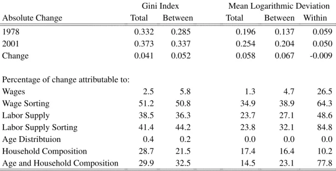
In this section, we examine several explanations for the rise in consumption inequality observed in the data. We focus on the years 1978 to 2001, as the major changes in inequality occurred over the 1980s. Results are presented in Table 6. The first two rows contain the benchmark inequality measures for 1978 and 2001, followed by the absolute change over time in the third row. The rest of the table presents the percentage of the change in the observed inequality measures attributed to each explanation we consider.
7.2.1 Wages and Labour Supply
According to the stylized facts, two of the most salient trends over time are the closing of the gender gap in wages and the rise in female labour supply. To what extent do changes in the distribution of wages account for the rise in consumption inequality? To answer this question, we conduct two exercises. In the first exercise, we start with the wage distribution in 2000. We then
re-weight the observations in the 1978 data so that the wage distribution in 1978 matches that of 2001. In particular, we construct histograms of log wages for 1978 and 2001. The histograms used to re-weight the wage distributions have 10 bins each. We re-weight 1978 data so that the histograms of log wages are the same in both years. This experiment captures the fall in the gender wage gap and aggregate changes in the wage distribution. In the second experiment, we focus on changes in the wage distributions within households. We re-weight the joint spousal distribution of wages in 1978 to match the joint spousal distribution of wages in 2000 to capture the effect of sorting on inequality. Both experiments are subsequently repeated for labour supply. The results are presented in Table 6.
What is interesting about the results on wage and hours sorting is that they can simultaneously explain both the rise in consumption inequality across households and the fall in consumption inequality within households: sorting on wages alone can explain approximately39% of the rise in between household inequality and 64% of the fall in within household inequality. It is also interesting to note that it is wage sorting within households in particular that is important, not changes to the aggregate wage distribution, as changes to the aggregate wage distribution explain little of the changes in inequality.
With respect to sorting on hours, 32% of the rise in between household inequality and 85% of the fall in within household inequality can be explained by increased marital sorting. Over time, the distribution of marriages shifted from ‘specialized’ families, with one income or a mix of low and high earners within the household, to a distribution with a larger proportion of both high earnings couples and low earnings couples. Regardless of the measure of consumption inequality considered, the exercises conducted above illuminate the dramatic role of sorting in determining the distribution of consumption across individuals. The evidence presented here is consistent with the existing literature on marital sorting and inequality that finds a positive relationship between marital sorting, on characteristics such as education, and inequality (Kremer, 1997; Dahan and Gaviria, 1999; Fernández and Rogerson, 2001; Fernández, Guner and Knowles, 2005).
7.2.2 Demographics and Household Composition
Next, we consider the hypothesis that the rise in consumption inequality is capturing cohort effects due to the changes in the age structure of the population. To this end, we re-weight the 1978 data so that the age structure is the same as that in 2001, holding all else constant. The results of this exercise, presented in the fifth row of the bottom panel of Table 6, suggest that changes in the age distribution between 1978 and 2001 had virtually no effect on consumption inequality. Thus, it does not appear that cohort effects are the driving force behind the trends in inequality.
The second explanation we consider is the large change in household composition that occurred alongside the rise in inequality. In particular, with delays in marriage and a rise in divorce rates, the fraction of households with one adult increased relative to the fraction of two adult households. Although single person households have no within household inequality by definition, it is still the case that there may exist substantial inequality between single adult households. To assess the importance of changing household composition, we re-weight the 1978 data so that the fraction of married couples, the fraction of single women, and the fraction of single men in the population match the proportions in 2001. The results of this exercise suggest that changes in household com-position can explain up to17%of the change in household inequality according to the sharing rule estimates and 16% of the change in consumption inequality when measured using adult equiva-lence scales. Together, a combination of a changing age distribution and the change in household composition over time can explain 14%of the change in the MLD over time, most of this effect coming through household composition. In summary, our experiments indicate that the main driv-ing force behind the trends in consumption inequality are changes in marital sortdriv-ing, not changes in demographics. This finding reaffirms the fact that our understanding of consumption inequality is incomplete when intra-household behavior is ignored.
8 Conclusion
The literature on consumption inequality has focused on the question of how changes in income inequality translate into changes in consumption inequality at the level of the individual. In this paper, we show that current measures of consumption inequality only reflect inequality at the household level, as it is assumed there is no inequality within households. We provide evidence that this assumption produces a very inaccurate picture of both the level and trend in consumption inequality for two reasons. First, the large dispersion in incomes in the household are highly in-consistent with equal division of consumption. When equal division is relaxed, there is substantial inequality within the household. This suggests previous work underestimates the level of individ-ual consumption ineqindivid-uality by30%. Second, the earnings gap within households has closed over the past 30 years, resulting in less inequality in the household over time. As a result, we estimate that the rise in inequality documented in the literature is overstated by 65%. Our results show that the conventional approach for measuring inequality is only appropriate for measuring inequality for single individuals and for couples with the same earnings.
Our work highlights the fact that looking inside the household is as important as looking be-tween households for the study of consumption inequality across individuals. What happens in the household not only changes our estimates of the level and trend in inequality; it also changes our understanding of the forces behind the trends. We find that increased marital sorting on earnings can explain both the fall in within household inequality and the rise in between household in-equality over time. These results are complementary to those of Fernández and Rogerson (2001), Fernández, Guner and Knowles (2005) and Dahan and Gaviria (2001), among others, on sorting and income inequality and suggest an important avenue for further research.
Table 1: Descriptive Statistics from the FES
Male Female
Single Married Single Married
1968 to 2001 Mean Std Dev Mean Std Dev Mean Std Dev Mean Std Dev
Age (22 to 65) 43.92 13.39 48.60 13.51 50.41 13.31 46.51 13.60
No hours dummy 0.28 0.45 0.19 0.40 0.43 0.49 0.35 0.48
Part time dummy 0.05 0.22 0.04 0.20 0.16 0.37 0.25 0.43 Full time dummy 0.68 0.47 0.77 0.42 0.41 0.49 0.40 0.49
Hourly wage 4.94 2.43 4.74 2.27 3.86 1.96 3.33 1.66
Total Expend. 118.37 99.10 192.51 129.48 99.53 75.63 192.51 129.48 Housing Expend. 39.57 41.62 59.61 62.93 39.07 37.91 59.61 62.93
Observations 10,958 31,871 12,967 31,871
Table 2: Estimates of the Preference Parameters.
Women Men
ρ 0.3919 0.3693 (0.0155) (0.0200)
α(at mean of data) 0.2314 0.2707
(0.0042) (0.0052) γ : Age 1.3298 2.5736 (0.0163) (0.0141) Age2 −2.4251 −4.8846 (0.0138) (0.0139) Education −0.1010 −0.0285 (0.0243) (0.0329) 1910 Cohort 0.6214 2.5868 (0.0176) (0.0084) 1920 Cohort 0.3903 1.5159 (0.0179) (0.0099) 1940 Cohort −0.4233 −1.2546 (0.0272) (0.0201) 1950 Cohort −0.7580 −1.5184 (0.0329) (0.0186) 1960 Cohort −0.8182 −1.9055 (0.0335) (0.0146) γ0 −1.2003 −0.9910 (0.0234) (0.0260) σ2 ν 0.6577 4.8676 (0.0526) (0.1478) corr(ν, u) 0.2448 0.1911 (0.0276) (0.0577)
Table 3: Estimates of the Sharing Rule.
Wives Husbands Restricted
φ0 −0.7729 −0.3011 −0.6645 (0.1176) (0.2233) (0.0954) φ1 2.5712 1.8491 2.3670 (0.2800) (0.5094) (0.2322) φ2 0.0031 0.0027 0.0022 (0.0025) (0.0026) (0.0017) φ0+12φ1+ 2.09φ2 0.5237 0.5192 0.6291 (0.0521) (0.0580) (0.0726) χ2(3) p-value φf =φm 6.4823 0.0905 t p-value φf0 =φm 0 −1.9491 0.0516 φf1 =φm 1 1.3436 0.1794 φf2 =φm 2 0.1572 0.8752
Table 4: Sharing Rule Estimates Under Alternative Measures of Public Goods
No Public Goods Public Goods (i) (housing) φ0 −0.1542 −0.1651 (0.0110) (0.0134) φ1 1.3805 1.3420 (0.0293) (0.0331) φ2 −0.0003 −0.0003 (0.0008) (0.0007) φ0+12φ1+ 2.09φ2 0.5354 0.5053 (0.0076) (0.0073) % of Total Consumption 0% 17%
Public Goods (ii) Public Goods (iii) (i + heat) (ii + durables +
transport + services) φ0 −0.1859 −0.1552 (0.0154) (0.0216) φ1 1.3845 1.4524 (0.0444) (0.0483) φ2 −0.0005 0.0042 (0.0010) (0.0019) φ0+12φ1+ 2.09φ2 0.5053 0.5798 (0.0216) (0.0208) % of Total Consumption 24% 56%
Table 5: Sharing Rule Estimates by Birth Cohort.
Birth Cohort Birth Cohort
1910 φ0 −0.8375 1920 φ0 −1.0278 N : 12,211 (0.1162) N: 18,660 (0.6900) φ1 2.8719 φ1 3.3587 (0.2968) (1.8565) φ2 0.0012 φ2 0.0023 (0.0021) (0.0065) φ0+12φ1+ 2.09φ2 0.6010 φ0+ 12φ1 + 2.09φ2 0.6564 (0.0773) (0.4725) 1930 φ0 −0.8417 1940 φ0 −0.2050 N: 16,219 (0.0722) N: 15,284 (0.0296) φ1 2.8238 φ1 1.1935 (0.2198) (0.0812) φ2 0.0017 φ2 0.0018 (0.0023) (0.0017) φ0+12φ1+ 2.09φ2 0.5738 φ0+ 12φ1 + 2.09φ2 0.3955 (0.0475) (0.0249) 1950 φ0 −0.8660 1960 φ0 −0.0529 N: 11,692 (0.2538) N: 7,974 (0.0704) φ1 2.6061 φ1 0.6802 (0.5621) (0.1692) φ2 0.0005 φ2 −0.0031 (0.0068) (0.0054) φ0+12φ1+ 2.09φ2 0.4381 φ0+ 12φ1 + 2.09φ2 0.2807 (0.0623) (0.0507)
Table 6: Decomposition of the Change in Between and Within Consumption Inequality.
Gini Index Mean Logarithmic Deviation
Absolute Change Total Between Total Between Within
1978 0.332 0.285 0.196 0.137 0.059
2001 0.373 0.337 0.254 0.204 0.050
Change 0.041 0.052 0.058 0.067 -0.009
Percentage of change attributable to:
Wages 2.5 5.8 1.3 4.7 26.5
Wage Sorting 51.2 50.8 34.9 38.9 64.3
Labor Supply 38.5 36.3 23.7 27.1 48.6
Labor Supply Sorting 41.4 44.2 23.8 32.1 84.8
Age Distribtuion 0.4 0.2 0.0 0.0 0.0
Household Composition 28.7 21.5 17.4 16.4 10.2
Individual Earnings
Household Earnings
Household Consumption
Adult Equivalent Consumption .3
.4 .5 .6 .7 Gini Coefficient .3 .4 .5 .6 .7 1970 1980 1990 2000 Year
Figure 1: Trends in the Gini index for earnings and consumption.
Note: Own calculations from the FES. Shaded area represents±two standard errors.
0
.1
.2
.3
Husband−wife earnings correlation
1970 1980 1990 2000
Year
Figure 2:Correlation in earnings across husbands and wives.
Actual Wage Share Potential Wage Share
.2 .25 .3 .35 .4 .45 1970 1980 1990 2000 Year
Figure 3:Fraction of actual household earnings provided by wife.
Note: Own calculations from the FES. Shaded area represents±two standard errors.
0 .2 .4 .6 0 .2 .4 .6 0 .2 .4 .6 0 .2 .4 .6 0 20 40 0 20 40 0 20 40 0 20 40
1968, Male, Single 1968, Male, Married 1968, Female, Single 1968, Female, Married
1978, Male, Single 1978, Male, Married 1978, Female, Single 1978, Female, Married
1988, Male, Single 1988, Male, Married 1988, Female, Single 1988, Female, Married
1998, Male, Single 1998, Male, Married 1998, Female, Single 1998, Female, Married
Fraction
Usual Weekly Hours Graphs by year, Sex, and Marital Status
Figure 4: Histogram of usual weekly hours.
All households Only one and two
adult households .25 .3 .35 .4 Gini Coefficient .25 .3 .35 .4 1970 1980 1990 2000 Year
Figure 5:Consumption inequality for all households and one- and two-adult households.
Note: UK National Statistics (1968–2001). Shaded area represents±two standard errors.
Total inequality Between household inequality .25 .3 .35 .4 .45 1970 1980 1990 2000 year Gini Coefficient Total inequality Between household inequality .1 .15 .2 .25 .3 .35 1970 1980 1990 2000 year
Mean Logarithmic Deviation
Figure 6:Total and between household decomposition of consumption inequality trends.
0 .2 .4 .6 .8 1
Lowest Rate/Top Rate
1970 1980 1990 2000
year
Lowest Rate Top Rate
Figure 7: Bottom and top marginal tax rates.
Source: UK National Statistics (1968–2001).
.8 1 1.2 1.4 1.6 1.8 .8 1 1.2 1.4 1.6 1.8
Mean Logarithmic Deviation, relative to 1968
1970 1980 1990 2000
year
Total inequality Between household inequality Within household inequality
Figure 8:Relative changes in between and within household inequality trends.
1968 2001 0 1 2 3 4 Kernel Density 0 .2 .4 .6 .8 1 Wife’s Share of Consumption
1968 2001 0 .2 .4 .6 .8 1 Cumulative Distribution 0 .2 .4 .6 .8 1 Wife’s Share of Consumption
References
ATTANASIO, O., E. BATTISTIN, AND H. ICHIMURA (2007): “What Really Happened to
Con-sumption Inequality in the US?,” inHard-to-Measure Goods and Services: Essays in Honor of Zvi Griliches, ed. by E. Berndt, andC. Hulten. The University of Chicago Press, NBER WP 10338.
BARRETT, G., T. CROSSLEY, ANDC. WORSWICK(2000): “Consumption and Income Inequality
in Australia,”Economic Record, 76(233), 116–138.
BATTISTIN, E. (2003): “Errors in survey reports of consumption expenditures,” available at
http://ideas.repec.org/p/ifs/ifsewp/03-07.html.
BLUNDELL, R., P.-A. CHIAPPORI, T. MAGNAC, AND C. MEGHIR (2007): “Collective Labour
Supply: Heterogeneity and Non-Participation,” Review of Economic Studies, 74(2), 417–445, available at http://ideas.repec.org/a/bla/restud/v74y2007i2p417-445.html.
BLUNDELL, R., P.-A. CHIAPPORI, AND C. MEGHIR (2005): “Collective Labor Supply with
Children,”Journal of Political Economy, 113, 1277–1306.
BLUNDELL, R., AND I. PRESTON (1998): “Consumption Inequality and Income Uncertainty,”
Quarterly Journal of Economics, 113(2), 603–640.
BROWNING, M., F. BOURGUIGNON, P.-A. CHIAPPORI, ANDV. LECHENE(1994): “Income and
Outcomes: A Structural Model of Intrahousehold Allocation,” Journal of Political Economy, 102(6), 1067–1096.
BROWNING, M., AND P.-A. CHIAPPORI(1998): “Efficient Intra-household Allocations: A
Gen-eral Characterization and Empirical Tests,”Econometrica, 66(6), 1241–1278.
BROWNING, M., P.-A. CHIAPPORI, AND A. LEWBEL (2006): “Estimating Consumption
Economies of Scale, Adult Equivalence Scales, and Household Bargaining Power,” Unpub-lished Manuscript.
CHIAPPORI, P.-A. (1988): “Rational Household Labor Supply,”Econometrica, 56(1), 63–90.
(1992): “Collective Labor Supply and Welfare,” Journal of Political Economy, 100(3), 437–467.
CUTLER, D., AND L. KATZ (1992): “Rising Inequality? Changes in the Distribution of Income
and Consumption in the 1980’s,”AEA Papers and Proceedings, 82(2), 546–551.
DAHAN, MOMI,ANDGAVIRIA, ALEJANDRO(2001): “Sibling Correlations and Intergenerational
Mobility in Latin America,”Economic Development and Cultural Change, 49(3), 537–554. DEPARTMENT OF EMPLOYMENT(1968–2001):Family Expenditure SurveyUK Data Archive,
DONNI, O. (2003): “Collective Household Labor Supply: Nonparticipation and Income Taxation,”
Journal of Public Economics, 87, 1179–1198.
(2007): “Collective Female Labor Supply: Theory and Application,”The Economic Jour-nal, 117, 94–119.
FERNÁNDEZ, R., N. GUNER, AND J. KNOWLES(2005): “Love and Money: A Theoretical and
Empirical Analysis of Household Sorting and Inequality,”The Quarterly Journal of Economics, 120(1), 273–344, available at http://ideas.repec.org/a/tpr/qjecon/v120y2005i1p273-344.html. FERNÁNDEZ, R., AND R. ROGERSON (2001): “Sorting and Long-Run Inequality,” Quarterly
Journal of Economics, 116(4), 1305–41.
GOULD, E. D., AND M. D. PASERMAN (2003): “Waiting for Mr. Right: rising inequality and
declining marriage rates,”Journal of Urban Economics, 53(2), 257–281.
HONG, J. H., AND J.-V. RÍOS-RULL (2007): “Life Insurance and Household Consumption,”
Journal of Monetary Economics, 54(1), 118–140.
HURST, E., AND A. LUSARDI (2004): “Liquidity Constraints, Household Wealth, and
En-trepreneurship,”Journal of Political Economy, 112(2), 319–347.
JOHNSON, D., AND S. SHIPP (1997): “Trends in Inequality using Consumption-Expenditures:
The U.S. from 1960 to 1993,”Review of Income and Wealth, 43(2), 133–152.
KREMER, M. (1997): “How Much Does Sorting Increase Inequality?,”The Quarterly Journal of
Economics, 112(1), 115–139.
KRUEGER, D., ANDF. PERRI(2006): “Does Income Inequality Lead to Consumption Inequality?
Evidence and Theory,”Review of Economic Studies, 73(1), 163–193.
LUNDBERG, S., R. POLLAK, AND T. WALES (1997): “Do Husbands and Wives Pool Their
Re-sources?,”The Journal of Human Resources, 32(3), 463–480.
MANSER, M.,ANDM. BROWN(1980): “Marriage and Household Decision Making: A bargaining
Analysis,”International Economic Review, 21(1), 31–44.
MAZZOCCO, M. (2004): “Savings, Risk Sharing and Preferences for Risk,” American Economic
Review, 94(4), 1169–1182.
(2007): “Household Intertemporal Behavior: a Collective Characterization and a Test of Commitment,”Review of Economic Studies, 74(3), 857–895.
MCELROY, M., AND M. HORNEY (1981): “Nash-Bargained Household Decisions: Toward A
Generalization of the Theory fo Demand,”International Economic Review, 22(2), 333–349. MCFADDEN, D., AND K. TRAIN(2000): “Mixed MNL Models for Discrete Response,”Journal