U.S. evolving macroeconomic dynamics: a structural investigation

(1)

WO R K I N G PA P E R S E R I E S

N O 7 4 6 / A P R I L 2 0 0 7

U.S. EVOLVING

MACROECONOMIC

DYNAMICS

A STRUCTURAL

INVESTIGATION

(2)

In 2007 all ECB publications feature a motif taken from the

€20 banknote.

W O R K I N G PA P E R S E R I E S

N O 7 4 6 / A P R I L 2 0 0 7

This paper can be downloaded without charge from http://www.ecb.int or from the Social Science Research Network electronic library at http://ssrn.com/abstract_id=978374.

U.S. EVOLVING

MACROECONOMIC

DYNAMICS

A STRUCTURAL

INVESTIGATION

I

by Luca Benati

2

and Haroon Mumtaz

3

(3)

© European Central Bank, 2007

Address Kaiserstrasse 29

60311 Frankfurt am Main, Germany

Postal address Postfach 16 03 19

60066 Frankfurt am Main, Germany

Telephone +49 69 1344 0 Internet http://www.ecb.int Fax +49 69 1344 6000 Telex 411 144 ecb d

Any reproduction, publication and reprint in the form of a different publication, whether printed or produced electronically, in whole or in part, is permitted only with the explicit written authorisation of the ECB or the author(s).

(4)

We fit a Bayesian time-varying parameters structural VAR with stochastic volatility to the Federal Funds rate, GDP deflator inflation, real GDP growth, and the rate of growth of M2. We identify 4 shocks–monetary policy, demand non-policy, supply, and money demand–by imposing sign restrictions on the estimated reduced-form VAR on a period-by-period basis. The evolution of the monetary rule in the structural VAR accords well with narrative accounts of post-WWII U.S. economic history, with (e.g.) significant increases in the long-run coefficients on inflation and money growth around the time of the Volcker disinflation. Overall, however, our evidence points towards a dominant role played by good luck in fostering the more stable macroeconomic environment of the last two decades. First, the Great Inflation was due, to a dominant extent, to large demand non-policy shocks, and to a lower extent to supply shocks. Second, imposing either Volcker or Greenspan over the entire sample period would only have had a limited impact on the Great Inflation episode, while imposing Burns and Miller would have resulted in a counterfactual inflation path remarkably close to the actual historical one. Although the systematic component of monetary policy clearly appears to have improved over the sample period, this does not appear to have been the dominant influence in post-WWII U.S. macroeconomic dynamics.

Keywords: Bayesian VARs; stochastic volatility; identified VARs; time-varying parameters; frequency domain; Great Inflation; Lucas critique.

(6)

Non Technical Summary

The U.S. ‘Great Moderation’–the dramatic decrease in macroeconomic volatility across the board of the last two decades–has been, in recent years, one of the most intensely investigated topics in macroeconomics. The stated goal of this strand of literature is to identify the relative contributions of two main candidates, good policy and good luck, in fostering the more stable macroeconomic environment of the most recent period. If the bulk of the stability of the post-Volcker stabilisation era were indeed to be attributed to the impact of improved monetary policy, we might then

be reasonably confident that macroeconomic instability is a memory of the past–

with the right monetary policy in place, the 1970s could never return. If, on the other hand, the current, more stable macroeconomic environment found its origin in the fact that, in recent years, the U.S. economy has been spared the large shocks of previous decades, even the best monetary policy would not necessarily shield the United States from a reappearance of macroeconomic turbulence.

In this paper wefit a Bayesian time-varying parameters structural VAR with

sto-chastic volatility to the Federal Funds rate, GDP deflator inflation, real GDP growth, and the rate of growth of M2, in order to investigate the evolution of both reduced-form properties, and, especially, structural characteristics of the U.S. economy over the post-1960 period. We identify 4 shocks–monetary policy, demand non-policy, supply, and money demand–by imposing sign restrictions on the estimated reduced-form VAR on a period-by-period basis, and we then investigate time-variation in sev-eral key aspects of the structure we recovered. Our main results may be summarised as follows.

The evolution of the long-run coeﬃcients of the structural monetary rule in the

VAR accords remarkably well with narrative accounts of post-WWII U.S.

macroeco-nomic history, with (e.g.) a comparatively less aggressive counter-inflationary stance

over the first part of the sample, and dramatic increases in the coeﬃcients on

in-flation and money growth around the time of the Volcker disinflation. Interestingly,

the FED’s counter-inflationary stance clearly appears to have temporarily decreased

around the time of both the 1990-1991 recession, and the most recent one, following the collapse of the dotcom bubble.

Overall, however–in line with the previous contributions of (e.g.) Primiceri

(2005), Sims and Zha (2006), and Gambetti, Pappa, and Canova (2006)–our ev-idence points towards a dominant role played by good luck in fostering the more

stable macroeconomic environment of the last two decades. First, the Great Inflation

was due, to a dominant extent, to large demand non-policy shocks, and to a lower extent to supply shocks. Second, ‘bringing Alan Greenspan back in time’ would only

have had a limited impact on the Great Inflation episode, with the maximum impact

on inflation equal to slightly more than three percentage points, at the cost of

signif-icantly lower output growth in the first part of the sample, especially in the second

half of the 1970s.

So, although the systematic component of monetary policy clearly appears to have

(7)

1

Introduction

The U.S. ‘Great Moderation’–the dramatic decrease in macroeconomic volatility across the board of the last two decades–has been, in recent years, one of the most

intensely investigated topics in macroeconomics.1 _{The stated goal of this strand of}

literature is to identify the relative contributions of two main candidates, good policy and good luck, in fostering the more stable macroeconomic environment of the most recent period. If the bulk of the stability of the post-Volcker stabilisation era were indeed to be attributed to the impact of improved monetary policy, we might then

be reasonably confident that macroeconomic instability is a memory of the past–

with the right monetary policy in place, the 1970s could never return. If, on the other hand, the current, more stable macroeconomic environment found its origin in the fact that, in recent years, the U.S. economy has been spared the large shocks of previous decades, even the best monetary policy would not necessarily shield the U.S. from a reappearance of macroeconomic turbulence.

In this paper wefit a Bayesian time-varying parameters structural VAR with

sto-chastic volatility to the Federal Funds rate, GDP deflator inflation, real GDP growth, and the rate of growth of M2, in order to investigate the evolution of both reduced-form properties, and, especially, structural characteristics of the U.S. economy over the post-1960 period. We identify 4 shocks–monetary policy, demand non-policy, supply, and money demand–by imposing sign restrictions on the estimated reduced-form VAR on a period-by-period basis, and we then investigate time-variation in sev-eral key aspects of the structure we recovered. Our main results may be summarised as follows.

• The evolution of the long-run coeﬃcients of the structural monetary rule in

the VAR accords remarkably well with narrative accounts of post-WWII U.S. macroeconomic history, with (e.g.) a comparatively less aggressive

counter-inflationary stance over the first part of the sample, and dramatic increases in

the coeﬃcients on inflation and money growth around the time of the Volcker

disinflation. Interestingly, the FED’s counter-inflationary stance clearly appears to have temporarily decreased around the time of both the 1990-1991 recession, and the most recent one, following the collapse of the dotcom bubble.

• Overall, however–in line with the previous contributions of Stock and

Wat-son (2002), Primiceri (2005), Sims and Zha (2006), and Canova and his co-authors–our evidence points towards a dominant role played by good luck in fostering the more stable macroeconomic environment of the last two decades.

First, the Great Inflation was due, to a dominant extent, to large demand

non-policy shocks, and to a lower extent to supply shocks. Second, ‘bringing Alan Greenspan back in time’ would only have had a limited impact on the Great

1_{See in particular Stock and Watson (2002), Ahmed, Levin, and Wilson (2004), Primiceri (2005),} Canova and Gambetti (2005), Gambetti, Pappa, and Canova (2006) and Sims and Zha (2006).

(8)

Inflation episode, with the maximum impact on inflation equal to slightly more

than three percentage points, at the cost of significantly lower output growth

in the first part of the sample, especially in the second half of the 1970s.

So, although the systematic component of monetary policy clearly appears to have

improved over the sample period, this does not appear to have been the dominant

influence in post-WWII U.S. macroeconomic dynamics.

From a methodological point of view, our paper improves upon previous studies based on time-varying parameters models along several dimensions. Primiceri (2005) only considers a Cholesky decomposition–which allows him to identify only a mon-etary policy shock–and in computing impulse-responses disregards the uncertainty originating from future time-variation in the VAR’s structure, which we instead tackle

via Monte Carlo integration. Both Canova and Gambetti (2005) and Gambetti,

Pappa, and Canova (2006), on the other hand, do not have a time-varying covariance

structure. While it is true that random-walk time-variation in the VAR’s coeﬃcients

introduces a form of heteroskedasticity in the model, a key problem is that, by

con-struction, it induces a close correlation between changes in the VAR’s coeﬃcients and

changes in the covariance structure, which a comparison between Cogley and Sargent (2002) and Cogley and Sargent (2005) clearly shows not to be in the data–at least

for the U.S.–and which, in general we have no reason to assume to hold.2

The paper is organised as follows. Section 2 discusses the reduced-form

speci-fication for the time-varying parameters VAR with stochastic volatility which we

use throughout the paper. Section 3 discusses key details of Bayesian inference–in particular, our choices for the priors, and the Markov chain Monte Carlo algorithm we use to simulate the posterior distribution of the hyperparameters and the states conditional on the data. Section 4 discusses time-variation in the reduced-form prop-erties of the economy since the second half of the 1960s, while Section 5 focusses on structural features. Section 6 concludes.

2

A Time-Varying Parameters VAR with

Stochas-tic Volatility

In what follows we work with the following time-varying parameters VAR(p) model:

Yt =B0,t+B1,tYt−1+...+Bp,tYt−p+ t≡X

0

tθt+ t (1)

where the notation is obvious, and Yt is defined as Yt ≡ [rt, πt, yt, mt]0, with rt, πt, yt, mtbeing the Federal funds rate, GDP deflator inflation, and the rates of growth 2_{In his comment on Cogley and Sargent (2002), Stock (2002) stresses how, if the data generation} process is characterised by a time-varying volatility structure, imposition of a constant covariance stucture automatically induces an upward bias in the estimated extent of parameters’ drift in the VAR, as the algorithm compensates for lack of time-variation in the covariance by ‘blowing up’ time-variation in the VAR’s coeﬃcients.

(9)

of real GDP and nominal M2, respectively (for a description of the data, see Appendix

A).3 _{The overall sample period is 1959:1-2005:4. For reasons of comparability with}

other papers in the literature4_{we set the lag order to}_p_{=2. Following, e.g., Cogley and}

Sargent (2002), Cogley and Sargent (2005), Primiceri (2005), and Gambetti, Pappa,

and Canova (2006) the VAR’s time-varying parameters, collected in the vectorθt, are

postulated to evolve according to

p(θt | θt−1, Q) =I(θt) f(θt | θt−1, Q) (2)

with I(θt) being an indicator function rejecting unstable draws–thus enforcing a

stationarity constraint on the VAR–and with f(θt | θt−1, Q)given by

θt=θt−1+ηt (3)

with η_t _∼ N(0, Q). The VAR’s reduced-form innovations in (1) are postulated to

be zero-mean normally distributed, with time-varying covariance matrix Ωt which,

following established practice, we factor as

Var( t)≡Ωt=At−1Ht(A−t1)0 (4)

The time-varying matrices Ht and At are defined as:

Ht≡ ⎡ ⎢ ⎢ ⎣ h1,t 0 0 0 0 h2,t 0 0 0 0 h3,t 0 0 0 0 h4,t ⎤ ⎥ ⎥ ⎦ At ≡ ⎡ ⎢ ⎢ ⎣ 1 0 0 0 α21,t 1 0 0 α31,t α32,t 1 0 α41,t α42,t α43,t 1 ⎤ ⎥ ⎥ ⎦ (5)

with thehi,t evolving as geometric random walks,

lnhi,t = lnhi,t−1+νi,t (6)

For future reference, we define ht ≡[h1,t, h2,t, h3,t, h4,t]0. Following Primiceri (2005),

we postulate the non-zero and non-one elements of the matrix At–which we collect

in the vectorαt≡[α21,t,α31,t, ..., α43,t]0–to evolve as driftless random walks,

αt=αt−1+τt , (7)

3_{GDP de}_fl_{ator in}_fl_{ation and the rates of growth of real GDP and nominal M2 have been computed} as the non-annualised quarter-on-quarter rates of growth of the relevant series. The Federal funds rate has then been rescaled in order to make it conceptually comparable with the other three series. Specifically, by defining the quarter-on-quarter and the annualised quarter-on-quarterfigures for the Federal Funds rate asrtandrAt, we havert=(1+rAt)1/4-1.

4_{See e.g. Cogley and Sargent (2002), Cogley and Sargent (2005), Primiceri (2005), and Gambetti,} Pappa, and Canova (2006).

(10)

and we assume the vector[u0t,η0t, τ0t,ν0t]0 to be distributed as ⎡ ⎢ ⎢ ⎣ ut ηt τt νt ⎤ ⎥ ⎥ ⎦∼N(0, V), with V = ⎡ ⎢ ⎢ ⎣ I4 0 0 0 0 Q 0 0 0 0 S 0 0 0 0 Z ⎤ ⎥ ⎥ ⎦ andZ = ⎡ ⎢ ⎢ ⎣ σ2 1 0 0 0 0 σ2 2 0 0 0 0 σ23 0 0 0 0 σ2 4 ⎤ ⎥ ⎥ ⎦ (8) where ut is such that t≡A−t1H

1 2

t ut. As discussed in Primiceri (2005), there are two

justifications for assuming a block-diagonal structure for Vt. First, parsimony, as

the model is already quite heavily parameterized. Second, ‘allowing for a completely

generic correlation structure among diﬀerent sources of uncertainty would preclude

any structural interpretation of the innovations’.5 _{Finally, following, again, Primiceri}

(2005) we adopt the additional simplifying assumption of postulating a block-diagonal

structure for S, too–namely

S _≡Var(τt) =Var(τt) = ⎡ ⎣ 0S2×11 0S1×22 0021××33 03×1 03×2 S3 ⎤ ⎦ (9)

with S1 ≡ Var(τ21,t), S2 ≡ Var([τ31,t, τ32,t]0), and S3 ≡ Var([τ41,t, τ32,t, τ43,t]0), thus

implying that the non-zero and non-one elements of At belonging to diﬀerent rows

evolve independently. As discussed in Primiceri (2005, Appendix A.2), this assump-tion drastically simplifies inference, as it allows to do Gibbs sampling on the non-zero

and non-one elements of At equation by equation.

We estimate (1)-(9)via Bayesian methods. The next section discusses our choices

for the priors, and the Markov-Chain Monte Carlo algorithm we use to simulate the posterior distribution of the hyperparameters and the states conditional on the data.

3

Bayesian Inference

We estimate (1)-(9) via Bayesian methods. The next two subsections describe our

choices for the priors, and the Markov-Chain Monte Carlo algorithm we use to sim-ulate the posterior distribution of the hyperparameters and the states conditional on the data, while the third section discusses how we check for convergence of the Markov chain to the ergodic distribution.

3.1

Priors

For the sake of simplicity, the prior distributions for the initial values of the states–

θ0,α0, andh0–which we postulate all to be normal, are assumed to be independent both from one another, and from the distribution of the hyperparameters. In order

(11)

to calibrate the prior distributions for θ0, α0 and h0 we estimate a time-invariant

version of (1) based on thefirst 8 years of data, from 1959 Q3 to 1966 Q4, and we set

θ0 ∼N h ˆ θOLS,4·Vˆ(ˆθOLS) i (10)

As forα0 andh0 we proceed as follows. LetΣˆOLS be the estimated covariance matrix

of t from the time-invariant VAR, and letC be the lower-triangular Choleski factor

of ΣˆOLS–i.e., CC0 = ˆΣOLS. We set

lnh0 ∼N(lnµ0,10×I3) (11)

where µ0 is a vector collecting the logarithms of the squared elements on the

diag-onal of C. We then divide each column of C by the corresponding element on the

diagonal–let’s call the matrix we thus obtain C˜–and we set

α0 ∼N[˜α0,V˜(˜α0)] (12)

whereα˜0–which, for future reference, we define asα˜0 ≡[˜α0,11, α˜0,21, ...,α˜0,61]0–is a vector collecting all the non-zero and non-one elements ofC˜−1_{(i.e, the elements below} the diagonal), and its covariance matrix, V˜(˜α0), is postulated to be diagonal, with

each individual (j,j) element equal to 10 times the absolute value of the corresponding

j-th element of α˜0. Such a choice for the covariance matrix ofα0 is clearly arbitrary,

but is motivated by our goal to scale the variance of each individual element ofα0 in

such a way as to take into account of the element’s magnitude.

Turning to the hyperparameters, we postulate independence between the

para-meters corresponding to the three matrices Q, S, and Z–an assumption we adopt

uniquely for reasons of convenience–and we make the following, standard

assump-tions. The matrix Q is postulated to follow an inverted Wishart distribution,

Q_∼IW¡Q¯−1, T0

¢

(13)

with prior degrees of freedom T0 and scale matrix T0Q¯. In order to minimize the

impact of the prior, thus maximizing the influence of sample information, we set T0

equal to the minimum value allowed, the length ofθtplus one. As for Q¯, we calibrate

it as Q¯= γ_×ΣˆOLS, setting γ=1.0×10−4, the same value used in Primiceri (2005), a

relatively ‘conservative’ prior compared to the 3.5_×10−4 _{used by Cogley and Sargent}

(2005).

The three blocks of S are assumed to follow inverted Wishart distributions, with

prior degrees of freedom set, again, equal to the minimum allowed, respectively, 2, 3 and 4: S1 ∼IW ¡_¯ S₁−1,2¢ (14) S2 ∼IW ¡_¯ S₂−1,3¢ (15) S3 ∼IW ¡_¯ S₃−1,4¢ (16)

(12)

As for S¯1, S¯2 and S¯3, we calibrate them based on α˜0 in (12) as S¯1=10−3 × |α˜0,11|,

¯

S2=10−3

×diag([_|α˜0,21|,|α˜0,31|]0) and S¯3=10−3×diag([|α˜0,41|,|α˜0,51|,|α˜0,61|]0). Such a

calibration is consistent with the one we adopted forQ, as it is equivalent to setting

¯

S1, S¯2 and S¯3 equal to 10−4 times the relevant diagonal block of V˜(˜α0) in (12). Finally, as for the variances of the stochastic volatility innovations, we follow Cogley and Sargent (2002, 2005) and we postulate an inverse-Gamma distribution for the elements of Z, σ2_i _∼IG µ 10−4 2 , 1 2 ¶ (17)

3.2

Simulating the posterior distribution

We simulate the posterior distribution of the hyperparameters and the states

condi-tional on the datavia the following MCMC algorithm, combining elements of

Prim-iceri (2005) and Cogley and Sargent (2002, 2005). In what follows, xt _{denotes the}

entire history of the vector x up to time t–i.e. xt

≡ [x0

1, x02, , x0t]0–while T is the sample length.

(a) Drawing the elements of θt Conditional onYT,αT, and HT, the observation equation (1) is linear, with Gaussian innovations and a known covariance matrix. Following Carter and Kohn (2004), the density p(θT|YT, αT, HT, V) can be factored as

p(θT_|YT, αT, HT, V) =p(θT|YT, αT, HT, V) T_Y−1

t=1

p(θt|θt+1, YT, αT, HT, V) (18)

Conditional on αT, HT, and V, the standard Kalman filter recursions nail down the

first element on the right hand side of (18), p(θT|YT, αT, HT, V) = N(θT, PT), with

PT being the precision matrix of θT produced by the Kalman filter. The remaining

elements in the factorization can then be computed via the backward recursion algo-rithm found, e.g., in Kim and Nelson (2000), or Cogley and Sargent (2005, appendix

B.2.1). Given the conditional normality of θt, we have

θt|t+1 =θt|t+Pt|tP_t−₊₁1_|_t(θt+1−θt) (19) Pt|t+1=Pt|t−Pt|tP_t−₊₁1_|_tPt|t (20) which provides, for each t from T-1 to 1, the remaining elements in (1), p(θt|θt+1, YT, αT, HT, V) = N(θt|t+1, Pt|t+1). Specifically, the backward recursion starts with a draw from N(θT, PT), call it ˜θT Conditional on ˜θT, (19)-(20) give us θT−1|T and PT−1|T, thus allowing us to draw ˜θT−1 from N(θT−1|T, PT−1|T), and so on untilt=1.

(b) Drawing the elements of αt Conditional on YT,θT, andHT, following

Prim-iceri (2005), we draw the elements of αt as follows. Equation (1) can be rewritten as

AtY˜t≡At(Yt-X

0

tθt)=At t ≡ut, with Var(ut)=Ht, namely

˜

(13)

˜

Y3,t =−α31,tY˜1,t−α32,tY˜2,t+u3,t (22)

˜

Y4,t =−α41,tY˜1,t−α42,tY˜2,t−α43,tY˜3,t+u4,t (23) –plus the identity Y˜1,t = u1,t–where [ ˜Y1,t, Y˜2,t,Y˜3,t,Y˜4,t]0 ≡ Y˜t. Based on the

ob-servation equations (21)-(23), and the transition equation (7), the elements of αt

can then be drawn by applying the same algorithm we described in the previous

paragraph separately to (21), (22) and (23). The assumption that S has the

block-diagonal structure (9) is in this respect crucial, although, as stressed by Primiceri (2005, Appendix D), it could in principle be relaxed.

(c) Drawing the elements of Ht Conditional on YT, θT, and αT, the orthogo-nalised innovations ut ≡ At(Yt-X

0

tθt), with Var(ut)=Ht, are observable. Following

Cogley and Sargent (2002), we then sample the hi,t’s by applying the univariate

al-gorithm of Jacquier, Polson, and Rossi (2004) element by element.6

(d) Drawing the hyperparameters Finally, conditional on YT_, _θT_, _HT_{, and} _αT_,

the innovations to θt, αt, the hi,t’s are observable, which allows us to draw the

hyperparameters–the elements of Q, S1, S2 S3, and the σ2i–from their respective

distributions.

Summing up, the MCMC algorithm simulates the posterior distribution of the

states and the hyperparameters, conditional on the data, by iterating on (a)-(d). In

what follows we use a burn-in period of 50,000 iterations to converge to the ergodic distribution, and after that we run 10,000 more iterations sampling every 10th draw

in order to reduce the autocorrelation across draws.7

3.3

Assessing the convergence of the Markov chain to the

ergodic distribution

Following Primiceri (2005), we assess the convergence of the Markov chain by inspect-ing the autocorrelation properties of the ergodic distribution’s draws. Specifically, in

what follows we consider the draws’ ineﬃciency factors (henceforth, IFs), defined as

the inverse of the relative numerical eﬃciency measure of Geweke (1992),

RN E= (2π)−1 1

S(0)

Z π

−π

S(ω)dω (24)

where S(ω) is the spectral density of the sequence of draws from the Gibbs sampler

for the quantity of interest at the frequencyω. We estimate the spectral densities by

smoothing the periodograms in the frequency domain by means of a Bartlett spectral window. Following Berkowitz and Diebold (1998), we select the bandwidth parameter

automatically via the procedure introduced by Beltrao and Bloomfield (1987).

6_{For details, see Cogley and Sargent (2005, Appendix B.2.5).}

7_{In this we follow Cogley and Sargent (2005). As stressed by Cogley and Sargent (2005), however,} this has the drawback of ‘increasing the variance of ensemble averages from the simulation’.

(14)

Figure 1 shows the draws’ IFs for the models’ hyperparameters–i.e., the free

elements of the matricesQ, Z, and S–and for the states, i.e. the time-varying

coef-ficients of the VAR (theθt), the volatilities (the hi,t’s), and the non-zero elements of

the matrix At. As the figure clearly shows, the autocorrelation of the draws is

uni-formly very low, being in the vast majority of cases around or below 3–as stressed by Primiceri (2005, Appendix B), values of the IFs below or around twenty are generally regarded as satisfactory.

4

Reduced-Form Evidence

Figures 2 to 7 show reduced-form evidence on the evolution of the U.S. economy since the second half of the 1960s–specifically, the time-varying elements ofΩt; the spectra,

normalised spectra and overall variance of inflation; the four series’ time-varying

overall predictability; and the standard deviations of k-step-ahead projections.

4.1

The evolution of

Ω

t

4.1.1 The Great Moderation and the evolution of ln_|Ωt|

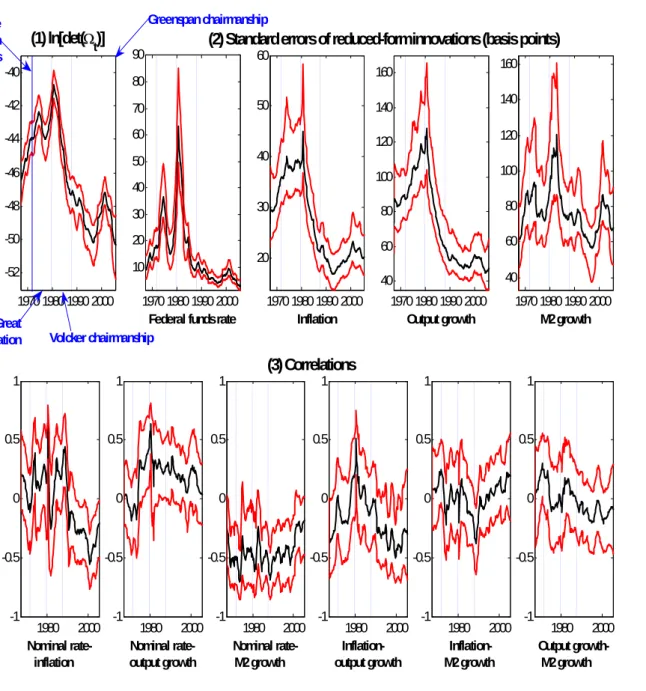
The top-left panel of Figure 2 provides a simple and stark illustration of the Great Moderation phenomenon, by plotting the median of the time-varying distribution of ln_|Ωt|, which, following Cogley and Sargent (2005),8 we interpret as a measure of the

total amount of noise ‘hitting the system’ at each point in time9_{–together with the}

16th and 84th percentiles.10 _ln

|Ωt|is estimated to have significantly increased around

the time of the Great Inflation episode,11 _{reaching a historical peak in 1980:2; to}

have dramatically decreased under the Chairmanship of Paul Volcker, and during the

8_{In turn, they were following Whittle (1953)–see Cogley and Sargent (2005, Section 3.5).} 9_{An anonymous referee pointed out that this ‘[...] can be misleading: suppose that the system} has two shocks which have high variance, but are nearly linearly dependent. Then log determinant of variance matrix will be very small, and yet the system may be very hard to predict.’ We entirely take this point, so it is important to be aware of the fact that these results suﬀer from this limitation. Unfortunately, it is not clear at all (at least, to us ...) how to eﬀectively solve this problem.

10_{Under normality, the 16th and 84th percentiles are the bounds of a one standard deviation} confidence interval, so that on average, for the normal distribution, the interval between these two percentiles encloses 68% of the distribution of the object of interest.

11_{Interestingly, the top-left panel of Figure 2 clearly suggests that the total prediction variance} started increasingbefore the collapse of Bretton Woods, in August 1971. There are two possible– and not mutually exclusive–interpretations of this result. First, from a strictly technical point of view, estimates of the states based on Gibbs sampling are, by construction, two-sided, and in the case of sharp breaks they therefore inevitably tend to ‘mix the future with the past’, thus giving the impression that the change took place before it actually did. Because of this, these results

are not incompatible with the notion that the increase in the total prediction variance actually

took place after August 1971. A second possibility is that these results are precisely capturing the macroeconomic turbulence that ultimately undid Bretton Woods–e.g. the large fiscal shocks associated with thefinancing of the Vietnam war.

(15)

first half of Alan Greenspan’s tenure; to have increased around the time of the 2000-2001 recession, thus testifying to the marked increase in macroeconomic turbulence associated with the unwinding of the dotcom bubble; and to have decreased ever since, reaching (based on median estimates) a historical low in the last quarter of the sample, 2005:4.

4.1.2 The other components of Ωt

Turning to the other components of Ωt, the remaining four panels in the top row

of Figure 2 show the evolution of the standard deviations of the VAR’s residuals, in basis points. For all four series, the volatility of reduced-form shocks reached a peak

around the time of the Volcker disinflation. This is especially clear for the Federal

Funds rate, which exhibited a dramatic spike corresponding to the FED’s temporary adoption of a policy of targeting non-borrowed reserves, between October 1979 and October 1982, but it is equally apparent, although in a less dramatic fashion, for the other three series.

The bottom row of Figure 2 shows the time-varying correlations between the four

reduced-form shocks. The sign of the correlation between shocks to inflation and to the

Federal Funds rate switched (based on median estimates) from predominantly positive

before the Volcker disinflation to negative thereafter. Although the interpretation

of this finding within the present non-structural setting is inevitably fraught with

hazards, such evidence is compatible with the notion that during the first half of the

sample the U.S. economy had been hit by large structural inflationary disturbances,

which caused inflation to shoot up, and monetary policy ‘to play catch-up’ with

inflation, thus inducing a positive correlation between the reduced-form shocks to

inflation and the Federal Funds rate. During the second half of the sample, on the

other hand, with the fall in the magnitude of structural inflationary disturbances, the

negative correlation between reduced-form shocks to the Federal Funds rate and to

inflation induced by structural monetary policy shocks became dominant. By contrast,

the correlation between reduced-form shocks to M2 growth and the Federal Funds

rate has remained comparatively quite remarkably stable,fluctuating around -0.5 for

the entire sample, with the only exception of the most recent years.

4.2

In

fl

ation’s variance and persistence

Figure 3 shows the logarithms of the medians of the distributions of the estimated

time-varying spectral densities of inflation, which following Cogley and Sargent (2005)

we approximate as fπ,t|T(ω) =sπ(I3−At|Te−iω)−1 Ωt|T 2π £ (I3 −At|Te−iω)−1 ¤0 s0π (25)

(where sπ is a row vector selecting inflation); the logarithms of the medians of the

(16)

inflation’s spectral density), together with the 16th and 84th percentiles; the medians of the distributions of the normalised spectrum computed based on (25); and the

median normalised spectrum atω=0, together with the 16th and 84th percentiles.

In line with Cogley and Sargent (2005) and Cogley and Sargent (2005), the data

generation process for U.S. inflation appears to have experienced two major changes

since the times of the Great Inflation. First, a dramatic reduction in inflation’s overall

variance, with the spectral density of inflation markedly decreasing at all frequencies

around the time of the Volcker disinflation; and inflation’s overall variance reaching a peak in 1980:2, systematically decreasing up until the end of Volcker’s Chairmanship,

and fluctuating at comparatively low levels under Chairman Greenspan. Second, a

fall in persistence coinciding, once again, with the Volcker disinflation episode. Based

on median estimates the normalised spectrum of inflation at ω=0 is estimated to

have fallen from a peak of 0.475 in 1975:1 to a low of 0.088 in 1985:1. After slightly

increasing during the second half of the 1980s, it has fluctuated, since mid-1992,

between 0.044 and 0.06.12 _{Given that, as it is well-known–see e.g. Granger and}

Newbold (1986) and Barsky (1987)–a stochastic process’ persistence is positively related to its extent of R2_{-forecastability, such marked fall in in}_fl_{ation persistence}

should automatically imply a corresponding decrease in inflation’s predictability. As

the next section shows, this has indeed been the case.

4.3

Assessing changes in the economy’s predictability

Following Cogley (2005), we measure changes in the four series’ predictability by

computing, for each of them, a time-varying multivariate R2 statistic on a

quarter-12_{A word of caution on the interpretation of persistence measures. As it is well known from the} work of, e.g., Pierre Perron–see in particular Perron (1989)–measuredpersistence crucially depends on the assumed specification for the mean (equilibrium component) of the process. Although in the present context we have postulated the equilibrium components of the three series to evolve smoothly over time, an alternative, and equally plausible, specification would be a step function– for an application to inflation within the univariate context, see e.g. Corvoisier and Mojon (2005). There are several reasons to prefer the present specification. First, and least important, for reasons of consistency with the previous literature, as the related work of Primiceri (2005), Canova and Gambetti (2005), and Gambetti, Pappa, and Canova (2006) has adopted the same specification. Second, and crucially, modelling the equilibrium components of the three series according to step functions would require afixed-coeﬃcients VAR with (some of the) coeﬃcients subject to structural breaks. Although, in principle, the break dates could be estimatedvia structural break tests–e.g., Bai and Perron (2003)–in practice both Cogley and Sargent (2005) and Benati (2007a) have shown such tests to possess a sometimes remarkably low power when the true DGP is characterised by random walk time variation. Time-varying parameters models, on the other hand, are well known for being capable of successfully tracking processes subject to structural breaks. As a consequence, while the ‘step function’ specification can be expected to perform well if and only if the DGP is subject to structural breaks, our specification can reasonably be expected to perform well under both scenarios.

(17)

is variable x’s estimated overall time-varying variance; fx,t|T(ω) is the time-varying

estimate of the spectral density of x based on the estimated time-varying VAR; and

σ2_,t_|_T = 2πexp ½ 1 2π Z π −π ln£fx,t|T(ω)dω ¤¾ (28)

is variable x’s estimated time-varying innovation variance, based on Kolmogorov’s

formula.

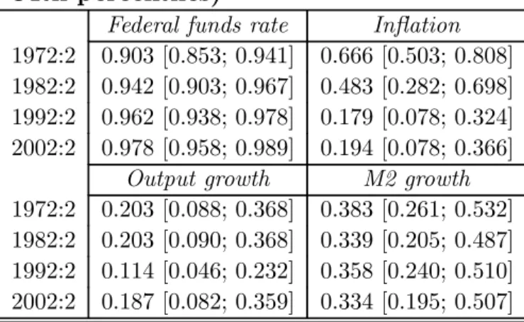
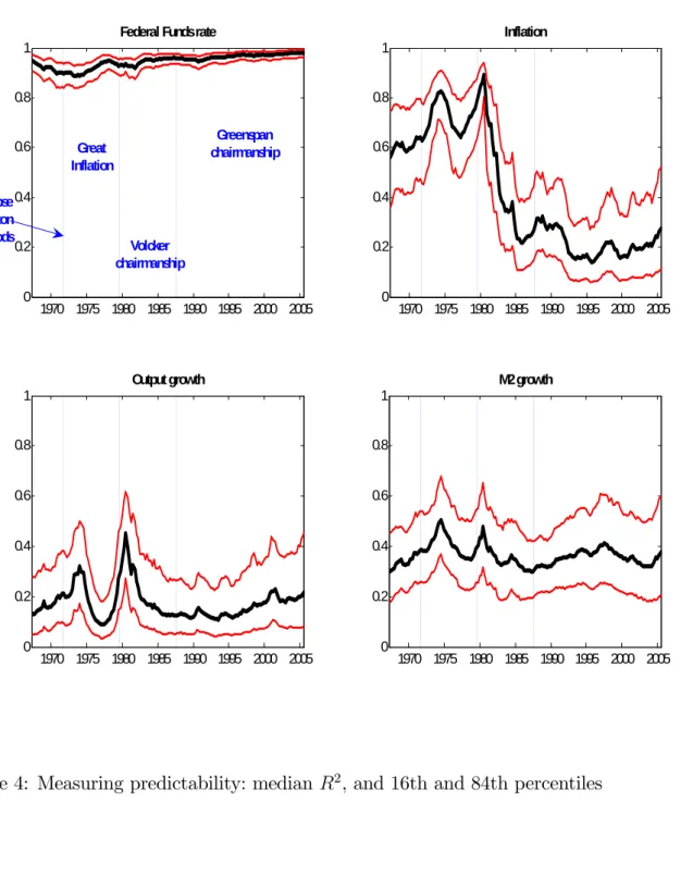
Figure 4 shows, for the four series, the medians of the distributions of the

time-varying multivariateR2 _{statistics, together with the 16th and 84th percentiles, while}

Table 1 reports the same objects for four selected quarters. As both thefigure and the

table make clear, the predictability of the Federal Funds rate has remained virtually

unchanged at values very close to one over the entire sample period,14 _{while M2}

growth’s forecastability has remained largely unchanged with the possible exception

of two mild spikes corresponding to the recession of the first half of the 1970s, and

to the Volcker recession. Output growth exhibits, overall, a pattern very similar to

that of M2 growth, with the main diﬀerences being, first, a uniformly lower overall

predictability, and second, a much more pronounced U-shape around the time of the Great Inflation, with a larger spike corresponding to the Volcker recession.15 _Finally,

consistent with the results for inflation persistence discussed in the previous section– and in line with the recent work of Stock and Watson (2007) documenting a decrease in U.S. inflation forecastability over the most recent years–inflation’s predictability is estimated to have reached (based on median estimates) a peak of 0.89 in 1980:2; to have dramatically declined during Volcker’s Chairmanship, reaching 0.27 at the end

of his tenure; and to have fluctuated at comparatively low levels, between 0.14 and

0.32, under Chairman Greenspan.

13_{Given the enormous computational burden associated with re-estimating the model every single} quarter, both this section’s exercise, and next section’s one, have been performed based on the smoothed (i.e, two-sided) output of the Gibbs samplerconditional on the full sample. This implies that both this section’s predictability measures, and next section’sk-step ahead projections, should only be regarded as approximations to the authentic out-of-sample objects that would result from a proper recursive estimation. (Unfortunately, it is not clear how to even gauge an idea of the goodness of such approximation.)

14_{This was in a sense to be expected, given that, as it is well known, the Federal Funds rate’s} behavior is close to a unit root.

15_{This was, again, to be expected, given that the Volcker recession has been the deepest and} longest since the times of the Great Depression.

(18)

Having discussed time-variation in the economy’s predictability, let’s now turn to the extent of uncertainty associated with future projections, as captured by the width and shape of model-generated ‘fan charts’ for the four series of interest.

4.4

Evolving macroeconomic uncertainty

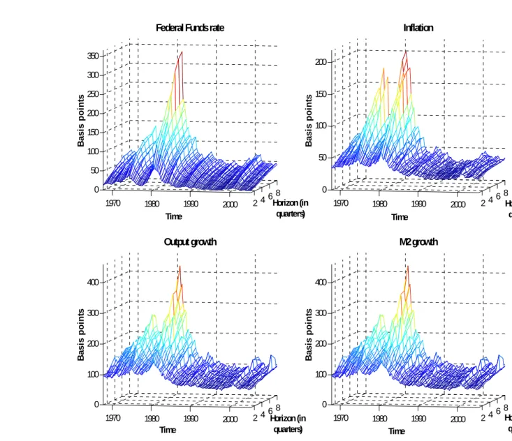
Figure 5 shows changes over time in the standard deviations (in basis points) of the

distributions of k-step-ahead forecasts for the four series of interest (for k = 1, 2,

..., 8 quarters), a simple measure of the extent of uncertainty associated with future projections, while Table 1 reports the same objects for four selected quarters and

three horizons.16 _{Projections have been computed by stochastically simulating the}

VAR into the future 1,000 times.17 As in the previous section, the present exercise

has been performed based on the two-sided output of the Gibbs sampler conditional

on the full sample, so that these k-step ahead projections should only be regarded

as approximations to the authentic out-of-sample objects that would result from a proper recursive estimation.

Several findings clearly emerge from Figure 5. First, consistent with the

discus-sion on the U.S. ‘Great Moderation’ of section 4.1, for all series, and at all horizons, the extent of uncertainty exhibits a very broadly similar hump-shaped pattern over the sample period, with peaks reached, depending on the series, in either 1980 or

1981, corresponding to the Volcker disinflation. After decreasing dramatically during

subsequent years for all series, and at all horizons, uncertainty has then fluctuated

at historically low levels ever since, with only mild and temporary increases corre-sponding to the 2000-2001 recession. Focussing on the two-year horizon–the one tra-ditionally associated with monetary policy decisions–the standard deviations of the

distributions of the projections for the Federal Funds rate, inflation, output growth,

and M2 growth have decreased from peaks of 332, 199, 419, and 375 basis points in 1980-1981 to 41, 35, 95, and 125 basis points in the last quarter of the sample, 2005:4, thus testifying to the dramatic decrease in macroeconomic uncertainty across the board over the last two decades and a half.

As for inflation, both the figure, and especially the table, clearly highlight the

impact on the extent of uncertainty surrounding its projections of two previously

discussed major changes which aﬀected its data generation process, a decrease in

both its persistence, and the volatility of its reduced-form innovations. While the decrease in the volatility of innovations caused a generalised downward shift in the

16_{In order to correctly interpret the information contained in the Figure and the Table, the reader} should keep in mind that inflation and the rates of growth of output and M2 have been computed as the non-annualised quarter-on-quarter rate of change of the relevant series, and that the Federal Funds rate has been rescaled accordingly.

17_Speci_fi_{cally, for every quarter, and for each of the 1,000 simulations, we start by sampling the} current state of the economy from the Gibbs sampler’s output for that quarter, by drawing a random number from a uniform distribution defined over [1; 1,000]. Conditional on this draw for the current state of the economy att, we then simulate the VAR 8 quarters into the future.

(19)

extent of uncertainty at all horizons, the fall in persistence ‘twisted’ the relationship between the forecast horizon and the standard deviation of the distribution of the

projections, making it flatter than it was around the time of the Great Inflation.18

A comparison between these results and those in the previous sub-section therefore clearly shows how–consistent with Stock and Watson (2007)–over the most recent

years U.S. inflation appears to have been, so far, less predictable than in the past

in the R2 sense, but, on the other hand, the extent of uncertainty associated with

inflation projection has drastically fallen, especially compared with the Great Inflation episode.

5

Structural Analysis

In the spirit of Primiceri (2005), Canova and Gambetti (2005), and Gambetti, Pappa, and Canova (2006), in this section we impose, on the estimated time-varying reduced-form VAR, identifying restrictions on a period-by-period basis. We identify four structural shocks–a monetary policy shock, a supply shock, a demand non-policy shock, and a money demand shock–based on sign restrictions.

5.1

Identi

fi

cation

Following Canova and de Nicolo (2002), Faust (1998), Peersman (2005), and Uhlig

(2005), our identification strategy relies on imposing the following sign restrictions

on the contemporaneous impacts of the structural shocks on the endogenous variable. We postulate

• the impact of a positive monetary policy shock to be non-negative on the interest

rate, and non-positive on inflation, and on the rates of growth of output and

M2;

• the impact of a demand non-policy shock be non-negative on all four variables.

• the impact of a supply shock be non-negative on output growth and non-positive

on inflation, while we leave its impact on the other two variables as

uncon-strained.

• the impact of a money demand shock be non-negative on both the interest rate

and M2 growth, and to be non-positive on both inflation and output growth.

18_{The easiest way to understand such changes is to focus on the limiting theoretical cases of a pure} random walk and of a pure white noise process. While for a random walk uncertainty (as measured by the conditional variance of the projection) increases linearly with the forecast horizon, for a pure whote noise process it is constant at all horizons.

(20)

It can be trivially shown that these restrictions are suﬃcient to uniquely identify

the four shocks. We compute the time-varying structural impact matrix, A0,t, via

the procedure recently introduced by Rubio-Ramirez, Waggoner, and Zha (2005).19

Specifically, let Ωt = PtDtPt0 be the eigenvalue-eigenvector decomposition of the VAR’s time-varying covariance matrixΩt, and let A˜0,t ≡PtD

1 2

t. We draw anN ×N

matrix,K, from theN(0, 1) distribution, we take the QRdecomposition of K–that

is, we compute matrices Q and R such that K=Q_·R–and we compute the

time-varying structural impact matrix asA0,t=A˜0,t·Q0. If the draw satisfies the restrictions we keep it, otherwise we discard it and we keep drawing until the restrictions are

sat-isfied, as in the Rubio-Waggoner-Zha code SRestrictRWZalg.m which implements

their algorithm.

5.2

The systematic component of monetary policy

5.2.1 The historical record

Figure 6 plots the medians and the 16th and 84th percentiles of the distributions of

the long-run coeﬃcients on inflation, output growth, and M2 growth in the

struc-tural monetary rule.20 _{Abstracting from the signi}_fi_{cant extent of econometric}

un-certainty, especially apparent in the second half of the sample, and focussing on

median estimates, the results reported in the figure accord, overall, quite

remark-ably well with traditional, ‘narrative’ accounts of post-WWII U.S. macroeconomic

history.21 Up to the arrival of Paul Volcker, U.S. monetary stance is estimated to

have been characterised by virtually no reaction to output growth; no reaction, or

a mildly negative reaction to M2 growth; and, most importantly, a comparatively

low reaction to inflation, estimated, during the Great Inflation episode, at slightly

below one.22 _{Volcker’s chairmanship appears instead to have been characterised by}

two major changes. First–in line with both ‘folk wisdom’, and traditional narrative

accounts–dramatic increases in the long-run coeﬃcients on both inflation and M2

growth.23 _{Second, a} _negative _coe_ﬃ_{cient on output growth around the time of the}

19_{See at http://home.earthlink.net/~tzha02/ProgramCode/SRestrictRWZalg.m.}

20_{We do not report the corresponding objects for the lagged Federal Funds rate as they are not} especially interesting, but they are available from the authors upon request.

21_{See in particular DeLong (1997).}

22_{An important point to stress is that the fact that the long-run coe}_ffi_{cient on in}_fl_{ation be–or} not be–above one should be drastically de-emphasised. As stressed by, e.g., Lubik and Schorfheide (2004), (in)determinacy is a system property–having to do with the interplay between all of the coefficients of the monetary rule and all of the structural coefficients of the model–and as such it bears no clear-cut relationship with the value taken by asingle (policy or non-policy) coefficient.

23_{As we already stressed in Section 4.1.1., because of the two-sided nature of Gibbs sampling’s} estimates, the fact that a specific object is estimated to have increased (decreased) over a period of several years isnot incompatiblewith the notion that, in reality, its change has been swift and sudden. So in the present case our estimates are compatible with the notion that the long-run coeﬃcients on inflation and M2 growth changed suddenly with the beginning of Volcker’s chairmanship.

(21)

Volcker disinflation, when the deepest recession since the Great Depression failed to

prevent further hikes in the Federal Funds rate.24 _{This is in line with the folk}

wis-dom about the Volcker disinflation as a decisive move to squeeze inflation out of the

system ‘no matter what’. Finally, the period since mid-1980s has been characterised by an overall declining weight on M2 growth; an overall increasing weight on output growth; and an overall slightly declining weight on inflation. Interestingly, the weight

on inflation clearly appears to have temporarily declined corresponding to the two

most recent recessions, the 1990-1991 one, coinciding with the first Gulf War, and

the one following the collapse of the dotcom bubble.25

Given that the evolution of the systematic component of monetary policy appears to have been in line with narrative accounts of post-WWII U.S. macroeconomic his-tory, a question naturally arises: ‘What if the most recent, stabilising monetary rule

had been in place around the time of the Great Inflation? Would it have been able

to save the day?’. Maybe surprisingly, as the next section shows the fact that U.S. monetary policy clearly appears to have improved compared with the pre-Volcker era

does not imply that the more recent monetary rule could have prevented the Great

Inflation at limited costs in terms of lost output.

5.2.2 Policy counterfactuals

Figures 7-9 shows results from a set of 1,000 counterfactual simulations in which we

have imposed, over the entire sample period, the structural monetary rules identified

for the Chairmanships26 _{of Arthur Burns and William Miller,}27_{Paul Volcker, and Alan}

Greenspan.28 _Speci_fi_{cally, the} _fi_{gures shows, for each of the four series, the medians}

of the distributions of the diﬀerence between the counterfactual paths and the actual

24_{It is important to remember, once again, that during the experiment with targeting} non-borrowed reserves (October 1979-October 1982) the Federal Funds rate was behaving like a market price, so that interest rates hikes were not purposefullyengineered by the FED, but they were rather

accepted.

25_{The results in the} _fi_{rst two panels of Figure 6 are qualitatively in line with those reported in} Kim and Nelson (2006)–see their Figures 2 and 3. Admittedly, though, Kim and Nelson’s Figure 3 is for the output gap, as opposed to output growth.

26_As _found _at _the _Federal _Reserve _Board’s _{website–see} _at

http://www.federalreserve.gov/bios/boardmembership.htm–the Chairmen’s tenures are the following. William McChesney Martin, Jr.: Apr. 2, 1951-Jan. 31, 1970; Arthur F. Burns: Feb. 1, 1970-Jan. 31, 1978; G. William Miller: Mar. 8, 1978-Aug. 6, 1979; Paul A. Volcker: Aug. 6, 1979-Aug. 11, 1987; Alan Greenspan Aug. 11, 1987-Jan. 31, 2006.

27_{Due to William Miller’s short tenure–just 17 months–we are ‘merging’ his Chairmanship with} Burns’.

28_Speci_fi_{cally, for each simulation}_j_{=1, 2, ...,}_N_{, at each quarter}_t₌_p_+1,_p_{+2, ...,}_T _{we draw three} random numbers,τ, indexing the quarter of the Chairmanship from which we draw the elements of the structural monetary rule; andκtandκτ, indexing the iterations of the Gibbs sampler at times tand, respectively,τ from which we draw the state of the economy. (All three numbers are defined over appropriate uniform distributions.) We then take all of the elements of the monetary rule from iterationκτ of the Gibbs sampler for quarterτ, while we take everything else from iterationκtfor

(22)

series, together with the 16th and 84th percentiles. Due to the limited number of observations available for the Chairmanship of William Martin (less than three years), we have chosen not to report the results from the counterfactual corresponding to this Chairman, but they are available upon request. Before delving into the results, an important point to mention is that, as it has been well known for a long time, structural VAR-based counterfactual simulations are, in principle, vulnerable to the Lucas critique, so that, in general, the results of this section should necessarily be

taken with a grain of salt.29 _{In a sub-section at the end of this paragraph we will}

therefore discuss to which extent Lucas critique-type problems can reasonably be thought to be relevant in the present context.

Starting with Figure 7, imposing Burns and Miller over the entire sample period produces three main results. First, the counterfactual Federal Funds rate is–not surprisingly–very close to the actual historical one up until the beginning of the

Volcker Chairmanship; the diﬀerence between the counterfactual path and the actual

series then decreases quite significantly under Volcker, reaching (based on median

estimates) a negative peak in excess of four percentage points around the time of the Volcker recession; and it then (very) slowly converges towards zero starting from mid-1980s. Second, the counterfactual inflation path is strikingly similar to the actual

one–if anything it is, quite surprisingly, very slightly lower than the actual one

around the time of the Volcker disinflation. Third, as it should be expected, output

growth is comparatively higher around the time of the 1980-1982 recession (by a maximum extent equal to about two percentage points), and it is still slightly higher

than the actual historical figure around the time of the 1990-1992 recession. Other

than that, however, the only non-negligible diﬀerence with historical outcomes is

around mid-1970s, when counterfactual output growth falls short of actual growth by about one percentage point. Overall, results from this counterfactual simulation clearly suggest, therefore, only a modest impact of policy on actual macroeconomic

outcomes, thus pointing towards luck, first bad, and then good, as the explanation

for the bulk of post-WWII U.S. macroeconomic dynamics.30

Turning to Figure 8, imposing Paul Volcker over the entire sample period produces

of the vectorYt.

It was pointed out by an anonymous referee that in this way ‘the policy coeﬃcients do not evolve smoothly [...], because now consecutive time periods [...] may receive policy coeﬃcients from non-consecutive periods’. This is certainly true, but the key issue here is that the ultimate goal of the counterfactual isnotto impose the Chairmen over the sample period in a way which is consistent with the specific way in which their chairmanships have historically evolved. Rather, it is to substitute (loosely speaking) an ‘average’ of the chairmanships over the entire sample.

29_{We wish to thank an anonimous referee for stressing the importance of this issue, and for} providing extremely useful suggestions.

30_{Based exactly on the same kind of logic, Benati (2007b) argues for a dominant role of good luck} in fostering the more stable macroeconomic environment of (roughly) the last two decades in the United Kingdom: if, by imposing the supposedly bad monetary rule of the 1970s over the entire sample period, basically nothing changes compared with actual historical outcomes, it necessarily has to be the case that policy did not play much of a role ...

(23)

two main results. First, virtually no diﬀerence, or very little diﬀerence, between ac-tual and counterfacac-tual outcomes over the period following the end of the Volcker

disinflation. Second, as for the years up to the end of the Volcker disinflation, it

generates counterfactual paths for inflation, output growth, and M2 growth

system-atically below actual historical ones. (It has to be stressed, however, that in the case

of inflation the diﬀerence is not enormous, reaching a maximum of about minus three

percentage points in the second half of the 1970s, when actual inflation was moving

towards ten per cent). Although this is exactly what we would have expected based

on Paul Volcker’s aggressively counter-inflationary reputation, what is at first sight

puzzling is that such disinflationary impact doesnot get achievedvia higher interest

ratesat any point in the sample, and especially during the very first few years. As the top-left panel clearly shows, indeed, up until 1976-1977 the counterfactual Federal Funds rate is broadly in line with the actual one, while during the years between

1976-1977 and the end of the Volcker disinflation the counterfactual rate is actually

lower than the historical one (by a maximum of about three percentage points in

1980Q1), thus suggesting that the lower counterfactual path for inflation translated,

via the Fisher eﬀect, into a lower path for interest rates. Given that higher

inter-est rates during the veryfirst years of the sample are not a possible explanation for

the systematically lower counterfactual paths for inflation, output growth, and M2

growth, the most logical explanation is, in our view, the expectational impact of the Volcker monetary rule.

Finally, turning to Figure 9, ‘bringing Alan Greenspan back in time’31 would have

had little impact on inflation before the collapse of Bretton Woods; it would have had

no discernible eﬀect after 1983-1984; and, most notably, it would have had a prolonged

discernible impact–equal, however, to at most slightly more than three percentage

points–between 1977 and 1981-1982, when inflation fluctuated between 5 and 11.6

per cent. As thefirst column shows, such a minor stabilising impact on inflation would

have been achievedvia higher interest rates, up to two additional percentage points,

in 1975-1977, and subsequently lower output and M2 growth during the second half of the 1970s.

How vulnerable are these results to the Lucas critique? In spite of the changes in the systematic component of monetary policy documented in the previous sub-section, overall, results from counterfactual simulations therefore suggest that

systematic monetary policy was not at the root of the Great Inflation episode, so

that either systematic policy mistakes, or just plain bad luck (e.g., large

non-31_{It was pointed out by an anonymous referee that, given the comparatively greater uncertainty} associated with the time-varying long-run coefficients in the structural monetary policy rule (see Figure 6: this is especially clear for the coefficient on inflation), ‘bringing Greenspan back in time means not only higher coefficients on inflation and money growth, but also much more volatile coefficients on inflation and money growth.’

(24)

policy shocks) must have been behind the inflationary upsurge of the 1970s.32 But how vulnerable are these results to the Lucas critique? Within a conceptually similar context, Sims and Zha (2006) raise indeed doubts on the reliability of the results reported in their Figure 8, depicting counterfactual paths for the Federal Funds rate,

output growth, and inflation conditional on an “inflation hawk Greenspan” with

doubled coeﬃcients on inflation in his monetary policy rule. In particular, they

question the reliability of the significant output losses generated by this simulation,

with the counterfactual path for output growth systematically and significantly below

the actual one until the beginning of the 1980s:

‘The counterfactual simulations that imply lower inflation create a

marked change in the stochastic process followed by output and inflation.

It is therefore quite possible that the output costs of the stronger

anti-inflationary policy stance would not have been so persistent as shown in

the graphs.’

In plain English, the output losses are so large that (i) they cannot be literally

believed, and (ii) they most likely results from Lucas critique-type problems. If, within the counterfactual, the full impact on expectations of the alternative monetary rule could have correctly been captured, the output losses would most likely be much lower.

Although solid within the context of the specific exercise Sims and Zha are

per-forming, such an argument appears (at least to to us) less so within the present

context, for the simple reason that, in two cases out of three, the diﬀerences between

actual and counterfactual paths are nowhere as nearly as dramatic as those depicted in Sims and Zha’s Figure 8 . Only in the case of the ‘Greenspan counterfactual’ of Figure 9 the output losses up to the end of the 1970s reach magnitudes comparable to

those generated by Sims and Zha’s “inflation hawk Greenspan”. Accordingly, in line

with Sims and Zha, these results should therefore be quite significantly discounted.

Figure 9, however, is not our only piece of evidence. In particular, as we previously stressed–and in line with Benati (2007b)–the fact that imposing the supposedly

‘bad’ monetary rule of the 1970s over the entire sample period (i) implies almost no

diﬀerence between the actual and counterfactual inflation paths, and (ii) it implies a

comparatively minor diﬀerence between the actual and counterfactual output growth

paths, represents, in our view, decisive evidence that the systematic component of

monetary policy did not play a significant role in generating the high macroeconomic

turbulence of the 1970s.

32_{Our overall conclusion is therefore in line with Sims and Zha’s (2006) that ‘[...] the estimated} policy changes do make a noticeable diﬀerence, but not a drastic diﬀerence.’

(25)

5.3

Structural variance decomposition

Figure 10 shows, for each of the four series, and for each single quarter, the

frac-tions of overall variance explained by each individual shock–specifically, the figure

shows the medians of the distributions of the fractions together with the 16th and 84th percentiles. The decomposition has been computed in the frequency domain, by

computing, for each quarter, each iteration of the Gibbs sampler, and each series x,

with x=rt,πt, yt,mt, both the series’ actual spectral density–fx,t|T(ω) in (27) and 28–and the four ‘counterfactual’ spectral densities obtained by setting to zero the

variances of each of the fours structural shocks but one.33 Given that a series’

vari-ance is equal to the integral of its spectral density, this trivially allows for a structural

decomposition of a series’ overall variance at each point in time.34

As the second row shows, demand non-policy shocks explained the lion’s share of the variance of inflation during the period up to the beginning of the Volcker disinfl a-tion, with (based on median estimates) the fraction of overall variance increasing from 40-50 per cent at the end of the 1960s to a peak in excess of 60 per cent around 1980. After falling below 40 per cent in 1981, the fraction of inflation’s variance due to

de-mand shocks continued to decline during subsequent years, and has beenfluctuating

between 10 and 20 per cent over the most recent period.35 By contrast, the fraction

due to policy shocks fluctuated around 10 per cent over the entire sample period–

with the exception of a short-lived spike up to about 20 per cent corresponding to

the Volcker disinflation–thus testifying, once again, to the negligible role played by

monetary policy in engineering the Great Inflation, even in itsnon-systematic

compo-nent. The influence of money demand shocks appears to have been likewise negligible

up to the end of the Volcker Chairmanship, but it has rapidly increased under Alan Greenspan, reaching almost 30 per cent at the end of the sample. Finally, the

frac-tion due to supply shocks fluctuated around 20 per cent until the beginning of the

Volcker disinflation, ‘it rapidly increased under Paul Volcker, and it had been fl uctu-ating, under Alan Greenspan, around 40 per cent. Taken together with the previous section’s findings, these results indicate that (i) the Great Inflation was due, to an overwhelming extent, to bad luck, i.e. to large non-policy shocks–in particular, to a

33_{An important point to stress is that while it can be easily shown that it is not possible to} uniquely identify the innovation variances of the four structural shocks, it is on the other hand possible to compute the (time-varying) covariance matrix of the VAR that would result from setting one (or more) of the structural innovation variances to zero.

34_{To put it di}_ﬀ_{erently, the sum of the four ‘counterfactual’ spectral densities is by construction} equal to the series’ actual spectral density,fx,t_|T(ω).

35_{As it was pointed out by a referee, ‘[i]t is possible that the weight of demand shocks in variance} decomposition of inflation and output has fallen exactly because monetary policy changed to less accommodating, and, in equilibrium, also private sector responses to such shocks diminished. If this is true, ‘Bringing Greenspan back in time’ would have a huge beneficial eﬀect.’. Here the problem is that the counterfactuals we performed in the previous sub-section do not support this hypothesis. To be fair, such counterfactuals are most likely subject to a Lucas critique argument, but then the issue becomes abandoning the SVAR methodology and using a DSGE model ...

(26)

dominant extent to demand shocks, and to a lower extent to supply shocks; and (ii) confronted with those large non-policy shocks, a more aggressive monetary rule like

Chairman Greenspan’s could have stabilised inflation only to a minor extent, and at

the price of significantly lower output growth in the second half of the 1970s.

Turning to the Federal Funds rate, thefirst column of Figure 10 shows that–quite

reassuringly ...–monetary policy shocks explain a comparatively minor fraction of the rate’s overall variance, with the bulk of the variation due instead to demand shocks, especially up until mid-1990s. The fraction due to supply shocks, on the other hand, remained relatively stable around 15-20 per cent over the entire sample period, with the exception of the most recent recession, when it temporarily shot up in excess of 40 per cent. Interestingly, the fraction of variance due to monetary policy shocks exhibits

a temporary spike in excess of 30 per cent corresponding to the Volcker disinflation

episode.

An analogous spike in excess of 30 per cent for monetary policy shocks

corre-sponding to the Volcker disinflation can be seen for output growth. Interestingly,

afterfluctuating quite erratically during the period up to 1987, the fraction of output

growth variance due to the non-systematic component of monetary policy stabilised, under Greenspan, around 10 per cent. Greenspan’s Chairmanship appears to have

been characterised by two other major phenomena: first, an analogous decrease in

the fraction of variance due to demand shocks; second, an higher fraction due to sup-ply shocks. Taken together, all these results are compatible with a view of monetary policymaking under Greenspan according to which the FED succeeded, to a greater extent than before, in keeping the economy close to the stochastic trend, minimising

the influence of demand shocks–either policy or non-policy–in driving output away

from potential, thus allowing supply shocks to dominate outputfluctuations.36

5.4

Changes in the transmission of monetary policy shocks

Although, historically, the non-systematic component of monetary policy appears to have explained only a minor fraction of the overall variance for all series except M2 growth, it might be of interest to explore how the transmission mechanism of monetary policy shocks has changed over time. Figure 11 plots, for the four series, the time-varying median generalised impulse-response functions (henceforth, IRFs) to a 25 basis points monetary policy shock, while Figure 12 shows the same objects, together with the16th and 84th percentiles of the distributions, for four selected dates.

Generalised IRFs have been computed via the Monte Carlo integration procedure

described in Appendix B, which allows to eﬀectively tackle the uncertainty originating

from future time-variation in the VAR’s structure. Due to the computational intensity of such a procedure, IRFs have been computed only every four quarters, starting from

36_{Another way of putting this is that the Greenspan FED, by keeping the economy closer to the} stochastic trend than before, caused it to behave, to a greater extent, like a real business cycle model.

(27)

Bothfigures clearly point towards an important change in the response of the Fed-eral Funds rate over the sample period, with a 25 basis points shock being followed,

over the first part of the sample, by negligible subsequent increases, and being

in-stead followed, over the most recent years, by comparatively larger subsequent hikes, building up, overall, up to about 40 basis points. It is also worth stressing how, during the second half of the 1970s, the contractionary impact of a interest rate hike

used to be partially oﬀset by a subsequent ‘reversal’, with the IRF becomingnegative

after about 6-8 quarters. Overall, these results are therefore fully consistent with the

findings of Section 5.2 of an improvement in the conduct of monetary policy

post-October 1979. Turning to the other three variables, once taking into account of the uncertainty surrounding median estimates (see Figure 12), it is not entirely clear that

IRFs have experienced significant changes over the sample period. The exception is

obviously represented by the very last portion of the sample, when the negative im-pact of a monetary policy shock increases dramatically for all the three variables, but one likely explanation for such results is simply that the very last quarters have just been imprecisely estimated.

6

A

Caveat

: The ‘Indeterminacy Hypothesis’

Taken at face value, our results clearly point towards good luck as the most plausible explanation for the greater macroeconomic stability of the most recent period. But

are there anycaveatsto ourinterpretationof these results? We believe that there is an

important one, which is currently being investigated in our related work in progress,37

and is extensively discussed in a companion paper on the Great Moderation in the

United Kingdom,38 to which the reader is referred to for further details.

Our point of departure is the striking contrast between the results from (time-varying parameters or Markov-switching) structural VARs, and those coming from an alternative, ‘narrative’ approach. As we previously discussed, the SVAR-based results of Stock and Watson (2002), Primiceri (2005), Sims and Zha (2006), and Canova and his co-authors suggest–in line with the present work–that plain good luck is the

key reason for the transition from the Great Inflation to the Great Moderation in

the United States. The narrative evidence, by contrast–see, in particular the work of DeLong (1997) and Romer and Romer (2002)–typically points towards improved

monetary policy, with the evolution of the U.S. monetary authority’s understanding

of the functioning of the economy being identified by the Romers as the main driver.

The contrast between the results coming from the two approaches is even more striking in the case of the United Kingdom. Although Benati (2007c), based on the

same methodology we used in the present work, identifies once again good luck as the

37_{Benati and Surico (2007).} 38_{Benati (2007c).}

(28)

explanation for the remarkable macroeconomic stability enjoyed by the U.K. economy

over the last two decades, as he discusses,39 _{his results stand in marked contrast with}

the narrative evidence produced