Classification of Hidden-Web Databases
LUIS GRAVANO and PANAGIOTIS G. IPEIROTIS Columbia University
and
MEHRAN SAHAMI Stanford University
The contents of many valuable Web-accessible databases are only available through search inter-faces and are hence invisible to traditional Web “crawlers.” Recently, commercial Web sites have started to manually organize Web-accessible databases into Yahoo!-like hierarchical classification schemes. Here we introduce QProber, a modular system that automates this classification process by using a small number of query probes, generated by document classifiers. QProber can use a variety of types of classifiers to generate the probes. To classify a database, QProber does not re-trieve or inspect any documents or pages from the database, but rather just exploits the number of matches that each query probe generates at the database in question. We have conducted an extensive experimental evaluation of QProber over collections of real documents, experimenting with different types of document classifiers and retrieval models. We have also tested our system with over one hundred Web-accessible databases. Our experiments show that our system has low overhead and achieves high classification accuracy across a variety of databases.
Categories and Subject Descriptors: H.3.1 [Content Analysis and Indexing]: Abstracting Methods; H.3.3 [Information Storage and Retrieval]: Information Search and Retrieval—
clustering, information filtering, search process, selection process; H.3.4 [Systems and Software]: Information Networks, Performance Evaluation (efficiency and effectiveness); H.3.5 [Information Storage and Retrieval]: Online Information Services—web-based services; H.3.7 [Information Storage and Retrieval]: Digital Libraries; H.2.4 [Database Management]: Systems—textual databases, distributed databases; H.2.5 [Database Management]: Systems—heterogeneous databases
General Terms: Algorithms, Experimentation, Performance
Additional Key Words and Phrases: Database classification, Web databases, hidden Web
This material is based upon work supported by the National Science Foundation under Grants No. IIS-97-33880 and IIS-98-17434. Any opinions, findings, and conclusions or recommendations expressed in this material are those of the authors and do not necessarily reflect the views of the National Science Foundation. P. G. Ipeirotis was partially supported by the Empeirikeio Foundation.
Authors’ addresses: L. Gravano and P. G. Ipeirotis, Computer Science Department, Columbia University, 1214 Amsterdam Ave., New York, NY 10027; email:{gravano;pirot}@cs.columbia.edu; M. Sahami, Computer Science Department, Stanford University, Stanford, CA 94305; email: [email protected].
Permission to make digital/hard copy of all or part of this material is granted without fee for per-sonal or classroom use provided that the copies are not made or distributed for profit or commercial advantage, the ACM copyright/server notice, the title of the publication, and its date appear, and notice is given that copying is by permission of the ACM, Inc. To copy otherwise, to republish, to post on servers, or to redistribute to lists requires prior specific permission and/or a fee.
C
1. INTRODUCTION
As the World-Wide Web continues to grow at an exponential rate, the problem of accurate information retrieval in such an environment also continues to es-calate. One especially important facet of this problem is the ability to not only retrieve static documents that exist on the Web, but also effectively determine which searchabledatabasesare most likely to contain the relevant information for which a user is looking. Indeed, a significant amount of information on the Web cannot be accessed directly through links, but is available only as a re-sponse to a dynamically issued query to the search interface of a database. The results page for a query typically contains dynamically generated links to these documents. Traditional search engines cannot index documents hidden behind such interfaces and ignore the contents of these resources, since they only take advantage of the link structure of the Web to “crawl” and index Web pages.
Even sites that have some links that are “crawlable” by a search engine may have much more information available only through a query interface, as the following real example illustrates.
Example 1.1. Consider the medical bibliographic database CANCERLITr
from the National Cancer Institute’s International Cancer Information Center, which makes medical bibliographic information about cancer available through
the Web.1If we query CANCERLIT for documents with the keywordslung AND
cancer, CANCERLIT returns 68,430 matches, corresponding to high-quality citations of medical articles. The abstracts and citations are stored locally at the CANCERLIT site and are not distributed over the Web. Unfortunately, the high-quality contents of CANCERLIT are not “crawlable” by traditional search
engines. A query2on AltaVista3that finds the pages in the CANCERLIT site
with the keywords “lung” and “cancer” returns 0 matches, which illustrates that the valuable content available through CANCERLIT is not indexable by traditional crawlers.
In addition, some Web sites prevent crawling by restricting access via a
robots.txtfile. Such sites then also become de facto noncrawlable.
In this article we concentrate onsearchable Web databasesoftextdocuments regardless of whether their contents are crawlable. More specifically, for our purposes a searchable Web database is a collection of text documents that is searchable through a Web-accessible search interface. The documents in a searchable Web database do not necessarily reside on a single centralized site, but can be scattered over several sites. Some searchable sites offer access to other kinds of information (e.g., image databases and shopping/auction sites); however, a discussion of the classification of these sites is beyond the scope of this article.
In order to effectively guide users to the appropriate searchable Web database, some Web sites (described in more detail below) have undertaken the arduous task of manually classifying searchable Web databases into a 1The query interface is available athttp://www.cancer.gov/search/cancer literature/. 2The query is
lung AND cancer AND host:www.cancer.gov.
Yahoo!-like hierarchical categorization scheme. Although we believe this type of categorization can be immensely helpful to Web users trying to find informa-tion relevant to a given topic, it is hampered by the lack of scalability inherent in manual classification. By providing an efficient automatic means for the accurate classification of searchable text databases into topic hierarchies, we hope to alleviate the scalability problems of manual database classification, and make it easier for end-users to find the relevant information they are seeking on the Web.
Consequently, in this article we describe our system, namedQProber, which
automates the categorization of searchable Web databasesinto topic hierarchies.
QProberuses a combination of machine learning and database querying
tech-niques. We use machine learning techniques to initially build document classi-fiers. Rather than actually using these classifiers to categorize individual doc-uments, we extract classificationrulesfrom the document classifiers, and we transform these rules into a set of query probes that can be sent to the search interface of the available text databases. Our algorithm then simply uses the number of matches reported for each query to make classification decisions,
without having to retrieve and analyze any of the actual database documents. This makes our approach very efficient and scalable.
The contributions presented in this article are organized as follows. In Section 2 we more formally define and provide various strategies for database classification. In Section 3 we present the details of our query probing algo-rithm for database classification and we describe a rule extraction algoalgo-rithm that can be used to extract query probes from a variety of both rule-based and linear document classifiers. In Sections 4 and 5 we provide the
exper-imental setting and results, respectively. We compare variations ofQProber
with existing methods for automatic database classification.QProberis shown to be both more accurate as well as more efficient on the database classifica-tion task. Also, we examine how different parameters affect the performance of QProber; we report results for the different types of classifiers used as well as results for different probing strategies and document retrieval mod-els. Section 6 describes related work, and Section 7 provides further discussion and outlines possible future research directions. Finally, Section 8 concludes the article.
2. CLASSIFICATION OF TEXT DATABASES
In this section we discuss how we can organize the space of searchable Web databases in a hierarchical categorization scheme. We first define appropri-ate classification schemes for such databases in Section 2.1, and then present alternative methods for text database categorization in Section 2.2.
2.1 Classification Schemes for Databases
Web directories like Yahoo! organize Web pages into categories for users to browse. In this section we extend this classification scheme to searchable Web databases and discuss classification alternatives.
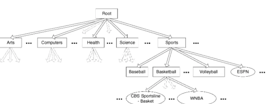
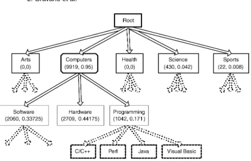
Fig. 1. Portion of the InvisibleWeb classification scheme.
Several commercial Web directories have recently started tomanually
clas-sify searchable Web databases, so that users can browse through these cate-gories to find the databases of interest. Examples of such directories include
InvisibleWeb4 and SearchEngineGuide.5 Figure 1 shows a small fraction of
InvisibleWeb’s classification scheme.
Formally, we can define a hierarchical classification scheme like the one used by InvisibleWeb as follows.
Definition 2.1. Ahierarchical classification schemeis a rooted directed tree whose nodes correspond to (topic) categories and whose edges denote special-ization. An edge from categoryv to another categoryv0 indicates thatv0 is a subcategory ofv.
Given a classification scheme, our goal is to automatically populate it with searchable databases where we assign each database to the “best” category or categories in the scheme. For example, InvisibleWeb has manually assigned WNBA to the“Basketball”category in its classification scheme. In general we can define what category or categories are “best” for a given database in several different ways, according to the needs the classification will serve. We describe these different approaches next.
2.2 Alternative Classification Strategies
We now turn to the central issue of how to automatically assign databases to categories in a classification scheme, assuming complete knowledge of the contents of these databases. Of course, in practice we will not have such com-plete knowledge, so we will have to use the probing techniques of Section 3 to approximate the “ideal” classification definitions that we give next.
To assign a searchable Web database to a category or set of categories in a classification scheme, one possibility is to manually inspect the contents of the database and make a decision based on the results of this inspection. Inciden-tally, this is the way in which commercial Web directories such as InvisibleWeb 4
http://www.invisibleweb.com.
operate. This approach might produce good quality category assignments but, of course, is expensive (it includes human participation) and does not scale well to the large number of searchable Web databases.
Alternatively, we could follow a less manual approach and determine the
category of a searchable Web database based on the category of thedocuments
it contains. We can formalize this approach as follows. Consider a Web database
Dandncategories,C1,. . .,Cn. If we knew the category of each of the documents insideD, then we could use this information to classify databaseDin at least two different ways. Acoverage-basedclassification will assignDto all categories for which Dhas sufficiently many documents. In contrast, aspecificity-based
classification will assignDto the categories that cover a significant fraction of
D’s holdings.
Example 2.2. Consider the topic category “Basketball.” CBS SportsLine
has a large number of articles about basketball and covers not only women’s basketball but other basketball leagues as well. It also covers other sports such
as football, baseball, and hockey. On the other hand,WNBAonly has articles
about women’s basketball. The way that we will classify these sites depends on the use of our classification. Users who prefer to seeonlyarticles relevant to basketball might prefer aspecificity-basedclassification and would like to have the siteWNBAclassified into node “Basketball.” However, these users would not want to haveCBS SportsLinein this node, since this site has a large number of articles irrelevant to basketball. In contrast, other users might prefer to have only databases with a broad and comprehensive coverage of basketball in the “Basketball” node. Such users might prefer acoverage-basedclassification and would like to findCBS SportsLinein the “Basketball” node, which has a large
number of articles about basketball, but notWNBAwith only a small fraction
of the total number of basketball documents.
More formally, we can use the number of documents in each category that we find in databaseDto define the following two metrics, which we use to specify the “ideal” classification ofD.
Definition 2.3. Consider a databaseD, a hierarchical classification scheme
C, and a category Ci ∈ C. The coverage of D for Ci, Coverage(D,Ci), is the number of documents inDin categoryCi:
Coverage(D,Ci)=number of D documents in category Ci.
Coverage(D,Ci) defines the “absolute” amount of information that database D contains about categoryCi.6
Definition 2.4. In the same setting as Definition 2.3, thespecificity of D for Ci,Specificity(D,Ci), is the fraction of documents in categoryCi inD. More 6It would be possible to normalizeCoveragevalues to be between 0 and 1 by dividing by the total number of
documents in categoryCi acrossalldatabases.Coveragewould then measure the fraction of the universally available information aboutCithat is stored inD. Alternatively, we could defineCoveragein terms of an idf-like measure to express the extent to which a database covers a topic that is rare overall. Although intuitively appealing, such definitions would be “unstable” since each insertion, deletion, or modification of a Web database would change theCoverageof the other available databases.
formally, we have:
Specificity(D,Ci)=
Coverage(D,Ci)
|D| ,
where|D|is the size of the database.
Specificity(D,Ci) gives a measure of how “focused” the database Dis on a category Ci. The value of Specificity ranges between 0 and 1. For notational convenience we define:
Coverage(D)=hCoverage(D,Ci1),. . .,Coverage(D,Cim)i
Specificity(D)=hSpecificity(D,Ci1),. . .,Specificity(D,Cim)i when the set of categories{Ci1,. . .,Cim}is clear from the context.
Now we can use theSpecificityandCoveragevalues to decide how to classify
Dinto one or more categories in the classification scheme. As described above, aspecificity-based classificationwould classify a database into a category when a significant fraction of the documents it contains are of this specific category. Alternatively, a coverage-based classificationwould classify a database into a category when the database has a substantial number of documents in the given category. In general, however, we are interested in balancing both Specificity
andCoveragethrough the introduction of two associated thresholdsτs andτc, respectively, as captured in the following definition.
Definition 2.5. Consider a classification scheme C with categories
C1,. . .,Cn, and a database D. The ideal classification of D in C is the set
Ideal(D) of categoriesCi that satisfy the following conditions. —Specificity(D,Ci)≥τs,
—Specificity(D,Cj)≥τsfor all ancestorsCj ofCi, —Coverage(D,Ci)≥τc,
—Coverage(D,Cj)≥τcfor all ancestorsCj ofCi, and
—Coverage(D,Ck) < τc or Specificity(D,Ck) < τs for each of the childrenCk ofCi,
where 0≤τs≤1 andτc≥1 are given thresholds.
The ideal classification definition given above provides alternative ap-proaches for “populating” a hierarchical classification scheme with searchable
Web databases, depending on the values of the thresholds τs and τc. A low
value for the specificity thresholdτswill result in a coverage-based classifica-tion of the databases. Similarly, a low value for the coverage thresholdτc will result in a specificity-based classification of the databases. The values chosen for τs andτc are ultimately determined by the intended use and audience of
the classification scheme.7 Next we introduce a technique for automatically
7The choice of thresholds might also depend on other factors. For example, consider a hypothetical
database with a “perfect” retrieval engine. Coverage might then be more important than specificity for this database if users extract information from the database by searching. The retrieval engine identifies exactly the on-topic documents for a query, making the presence of off-topic documents
populating a classification scheme according to the ideal classification of choice.
3. CLASSIFYING DATABASES THROUGH PROBING
In the previous section we defined how to classify a database based on the num-ber of documents that it contains in each category. Unfortunately, databases typically do not export such category-frequency information. In this section we describe how we can approximate this information for a given database with-out accessing its contents. The whole procedure is divided into two parts: First we train our system for a given classification scheme and then we probe each database with queries to decide the categories to which it should be assigned. More specifically, we follow the algorithm below.
(1) Train a document classifier with a set of preclassified documents (Section 3.1).
(2) Extract a set of classificationrulesfrom the document classifier and trans-form classifier rules into queries (Sections 3.2 and 3.3).
(3) Adaptively issue queries to databases, extracting and adjusting the num-ber of matches for each query using the classifier’s “confusion matrix” (Section 3.4).
(4) Classify databases using the adjusted number of query matches (Section 3.5).
3.1 Training a Document Classifier
Our database classification technique relies on a document classifier to create the probing queries, so our first step is to train such a classifier. We use super-vised learning to construct the classifier from a set of preclassified documents. The procedure follows a sequence of steps, described below.
The first step, which helps both efficiency and effectiveness, is to eliminate from the training set all words that appear very frequently in the training documents, as well as very infrequently appearing words. This initial “feature selection” step is based on Zipf ’s law [Zipf 1949], which provides a functional form for the distribution of word frequencies in document collections. Very fre-quent words are usually auxiliary words that bear no information content (e.g., “am,” “and,” “so” in English). Infrequently occurring words are not very helpful for classification either, because they appear in so few documents that there are no significant accuracy gains from including such terms in a classifier.
The elimination of words dictated by Zipf ’s law is a form of feature selection. However, frequency information alone is not, after some point, a good indicator to drive the feature selection process further. Thus we use an information-theoretic feature selection algorithm that eliminates the terms that have the
in the database irrelevant. Then the “perceived specificity” of the database for a given category for which it has sufficientCoverageis 1, which would argue for the use of a coverage-based classification of the database.
least impact on the class distribution of documents [Koller and Sahami 1997, 1996]. This step eliminates the features that either do not have enough dis-criminating power (i.e., words that are not strongly associated with one specific category) or features that are redundant given the presence of another feature. Using this algorithm we decrease the number of features in a principled way and we can use a much smaller subset of words to create the classifier, with min-imal loss in accuracy. In addition, the remaining features are generally more useful for classification purposes, so classifiers constructed from these features will tend to include more meaningful terms.
After selecting the features (i.e., words) that we will use for building the document classifier, we can use an existing machine learning algorithm to create a document classifier. Many different algorithms for creating document classifiers have been developed over the last few decades. Well-known tech-niques include the Naive Bayes classifier [Duda and Hart 1973], C4.5 [Quinlan 1992], RIPPER [Cohen 1996], and Support Vector Machines [Joachims 1998], to name just a few. These document classifiers work with a flat set of categories. To define a document classifier over an entire hierarchical classification scheme (Definition 2.1), we train one flat document classifier for eachinternalnode of the hierarchy.
Once we have trained a document classifier, we could use it to classify all thedocumentsin a database of interest to determine the number of documents
about each category in the database. We could then classify the database
it-self according to the number of documents that it contains in each category, as described in Section 2. Of course, this requires having access to the whole con-tents of the database, which is not a realistic requirement for Web databases. We relax this requirement presently.
3.2 Defining Query Probes from a Rule-Based Document Classifier
In this section we first describe the class ofrule-based classifiersand then we show how we can use a rule-based classifier to generate a set ofquery probes
that will help us estimate the number of documents for each category of interest in a searchable Web database.
In a rule-based classifier, the classification decisions are based on a set of logical rules; the antecedents of the rules are conjunctions of words and the consequents are the category assignments for documents. For example, the following rules are part of a classifier for the three categories “Sports,” “Health,” and “Computers.”
ibm AND computer→Computers jordan AND bulls→Sports diabetes→Health
cancer AND lung→Health intel→Computers
Such rules are used to classify previously unseen documents (i.e., documents not in the training set). For example, the first rule would classify all documents containing the words “ibm” and “computer” into the category “Computers.”
Definition 3.1. Arule-based document classifierfor aflatset of categories
C= {C1,. . .,Cn}consists of a set of rules pk→Clk,k =1,. . .,m, wherepk is a conjunction of words andClk ∈C. A documentd matches a rule pk→Clk if all the words in that rule’s antecedentpkappear ind. If a document matches mul-tiple rules with different classification decisions, the final classification decision depends on the specific implementation of the rule-based classifier.
We can simulate the behavior of a rule-based classifier over all documents of a database by mapping each rule pk → Clk of the classifier into a Boolean queryqk that is the conjunction of all words in pk. Thus if we send the query probeqkto the search interface of a database D, the query will match exactly the f(qk) documents in the databaseDthat would have been classified by the associated rule into categoryClk. For example, we map the rulejordan AND
bulls→Sportsinto the Boolean queryjordan AND bulls. We expect this query to retrieve mostly documents in the“Sports”category. Now instead of retrieving the documents themselves, we just keep the number of matches reported for this query (it is quite common for a database to start the results page with a
line such as “X documents found”), and use this number as a measure of how
many documents in the database match the condition of this rule.
From the number of matches for each query probe, we can construct a good ap-proximation of theCoverageandSpecificityvectors for a databaseD(Section 2).
We can approximate the number of documents inDin categoryCi as the total
number of matches from all query probes derived from rules with categoryCi
as a consequent. Using this information we can approximate theCoverageand
Specificityvectors for Das follows.
Definition 3.2. Consider a searchable Web database D and a rule-based
classifier for a set of categoriesC. For each query probeqderived from the clas-sifier, databaseDreturns the number of matches f(q). Theestimated coverage of D for a category Ci ∈C,ECoverage(D,Ci), is the total number of matches for theCi query probes.
ECoverage(D,Ci) =
X
qis a query probe forCi
f(q).
Definition 3.3. In the same setting as Definition 3.2, theestimated speci-ficity of D for Ci,ESpecificity(D,Ci), is
ESpecificity(D,Ci) =
ESpecificityP (D,Parent(Ci))·ECoverage(D,Ci) Cjis a child of Parent(Ci)ECoverage(D,Cj)
.
As a special case,ESpecificity(D, “root”)=1.
Thus, Definition 3.3 tells us that the estimated specificity for a categoryCiinD is the estimated percentage of documents inDthat are inParent(Ci) multiplied by the percentage of documents inParent(Ci) that are also inCi.
For notational convenience we define:
ECoverage(D) = hECoverage(D,Ci1),. . .,ECoverage(D,Cim)i
ESpecificity(D) = hESpecificity(D,Ci1),. . .,ESpecificity(D,Cim)i when the set of categories{Ci1,. . .,Cim}is clear from the context.
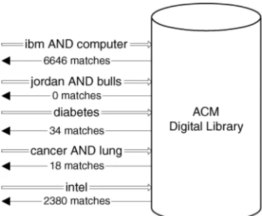
Fig. 2. Sending probes to the ACM Digital Library database with queries derived from a document classifier.
Example 3.4. Consider a small rule-based document classifier for
cate-gories C1 = “Sports,”C2 = “Computers,” andC3 =“Health” consisting of the five rules listed previously. Suppose that we want to classify the ACM Digital
Library database. We send the queryibm AND computer, which results in 6646
matching documents (Figure 2). The other four queries return the matches described in Figure 2. Using these numbers we can estimate that the ACM
Digital Library has 0 documents about “Sports,” 6646+2380=9026
docu-ments about “Computers,” and 18+34=52 documents about “Health.” Thus
theECoverage(ACM) vector for this set of categories is:
ECoverage(ACM)=(0, 9026, 52) and the respectiveESpecificity(ACM) vector is:
ESpecificity(ACM)= µ 0 0+9026+52, 9026 0+9026+52, 52 0+9026+52 ¶ .
As defined above, the computation ofECoveragemight count documents more
than once, since the same document might match multiple query probes. To ad-dress this issue, we could issue query probes in order, augmenting each query probe with the negation of all earlier query probes. Consider the five
exam-ple rules above, in the order they are listed. The first query would be ibm
AND computer, as before. However, the second query becomes jordan AND
bulls AND NOT(ibm AND computer), to not match (and count) any document
that matches the first query probe. This technique ensures that the final num-ber of matches for each category is not artificially inflated by documents that match multiple query probes. Unfortunately, if implemented in a naive way, this overlap-elimination strategy may result in rather long query probes, which might not be accepted by the databases. This problem could be partially solved by “breaking” the long queries into smaller conjunctive queries. Then, by ex-ploiting the inclusion-exclusion principle and the number of matches for each of the smaller probes, we can calculate the number of matches for the complex
query. For example, instead of sending the queryjordan AND bulls AND NOT
AND bullsand then subtract from it the number of matches generated for the
queryjordan AND bulls AND ibm AND computer. Unfortunately, the
num-ber of probes needed for this strategy increases exponentially with the query length. In Section 5 we experimentally evaluate the benefits of this expensive overlap-elimination strategy.
3.3 Extracting Query Probes from Numerically Parameterized Document Classifiers
We have seen so far that we can directly use a rule-based classifier to generate the query probes required for our database classification technique. However,
restricting QProber to only rule-based classifiers would prevent us from
ex-ploiting other classification strategies as they are developed. In this section, we describe how we can adapt numerically parameterized classifiers for use with
QProber. In particular we describe an algorithm that approximates a linear bi-nary classifier with a set of classification rules. We also describe briefly how the same algorithm can be modified to approximate different types of classifiers. Finally, we give some pointers to existing work in the area of rule extraction. Before describing the algorithm in detail, we define the terminology that we use.
Definition 3.5. A binary classifier decides whether a document,
repre-sented using m features (i.e., words), belongs to one class or not. A binary
linear classifiermakes this decision by calculating, during the training phase,
mweightsw1,. . .,wm and a thresholdbdetermining a hyperplane such that all pointst = ht1,. . .,tmiin the hyperplane satisfy the equation:
m
X
i=1
witi =b. (1)
This hyperplane divides them-dimensional document space into two regions:
the region with the documents that belong to the class in question, and the region with all other documents. Then, given them-dimensional representation
hs1,. . .,smiof a document [Salton and Buckley 1988], the classifier calculates the document’s “score” asPmi=1wisi. The value of this score relative to that of thresholdbdetermines the classification decision for the document.
A large number of classifiers fall into the category of linear classifiers. Examples include Naive Bayes and Support Vector Machines (SVM) with lin-ear kernel functions. Details on how to calculate these weights for SVMs and for Naive Bayesian classifiers can be found in Burges [1998] and in Nilsson [1990], respectively. A classifier fornclasses can be created usingnbinary clas-sifiers, one for each class. Note that such a composite classifier may result in a document being categorized into multiple classes or into no classes at all.
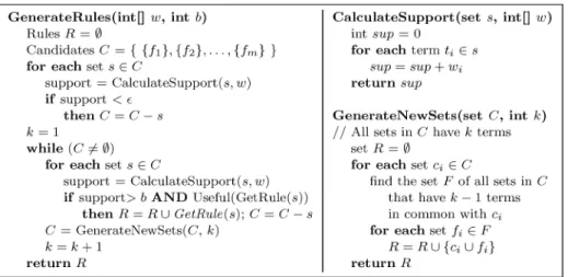
We can use Equation (1) to approximate a linear classifier with a rule-based classifier that will be used to generate the query probes. The intuition be-hind the rule-extraction algorithm that we introduce next is that the presence of a few highly weighted terms in a document suffices for the linear classi-fier to make a positive decision (i.e., go above threshold). Our rule-extraction
Fig. 3. Generating rules from a set of weightswiand a thresholdb.
algorithm works by generating rules iteratively. In each iteration we create rules of different length, that is, with a different number of terms in the an-tecedents. During the first iteration, we consider only rules with one term. If the weight of a term is higher than the threshold b, then this term is quali-fied to form a rule, since the presence of this term alone suffices to classify a document into the category. For efficiency and simplicity, the rules are formed as conjunctions of terms with no negations. After creating all the rules with one term, the algorithm proceeds to the next iteration, in which it creates rules with two terms, and so on.
The algorithm is described in more detail in Figure 3. In general, a sufficient condition for a set of terms to form a rule is that the sum of the weights of its terms exceeds the value of the threshold b, when all weights defining the separating hyperplane are nonnegative. Although the classifiers we consider do not necessarily produce exclusively nonnegative weights, we nevertheless find that our sufficiency criteria for extracting rules works reasonably well, since the term weights generally tend to be nonnegative.
Also, the derived rule has to be “useful”: a rule is useful if and only if it covers a given number of examples from the training set and its precision is greater than 0.5 (i.e., it matches more correct documents than incorrect ones). The terms that form a rule are removed from further consideration and will not participate in later iterations of the algorithm. Also, training examples that match a produced rule are removed from the training set, and will not be used in later iterations. To proceed to the next iteration, the algorithm expands unused term sets by one term, in a spirit similar to an algorithm for finding “association rules” [Agrawal and Srikant 1994]. In our algorithm, the “support” of a set of terms is defined as the sum of the weights of its terms, and the objective is to extend the “small” itemsets (i.e., the sets of terms whose sum of weights is smaller thanb) to get new itemsets with larger support.
Our rule extraction algorithm can be used for classifiers that divide the space using a nonlinear polynomial as well. For example, SVMs with polynomial
kernels can be treated in a similar way by considering the weights associated with all the higher-order terms in the function, but in this case the possible combinations of terms that need to be considered is greatly increased.
The task of rule extraction from classification models that do not explicitly represent their output as rules has been studied extensively in the machine learning community. A typical example is the C4.5RULES algorithm [Quinlan 1992], which generates a set of production rules from a decision tree. Another example is TREPAN[Craven 1996], which extracts a comprehensible set of rules from a neural network. Flake et al. [2002] describe an algorithm for extraction of rules from nonlinear SVMs. The ongoing research in rule extraction can be directly leveraged to adapt different learning models for use withQProber. 3.4 Adjusting Probing Results
QProber relies on document classifiers to define query probes and obtain
category-frequency information for a database. Unfortunately, document classifiers are not perfect because they can misclassify documents into incorrect categories, and leave any documents that do not match any rules unclassified. In this section we present a novel algorithm to adjust our initial probing results to account for such potential errors.
It is common practice in the machine learning community to report document classification results using aconfusion matrix[Kohavi and Provost 1998]. We adapt this notion of a confusion matrix for use in our probing scenario.
Definition 3.6. Thenormalized confusion matrix M=(mij) of a set of query probes for categoriesC1,. . .,Cnis ann×nmatrix, wheremijis the sum of the
number of matches generated from documents in categoryCj for categoryCi
query probes, divided by the total number of documents in categoryCj. In a perfect setting, the probes for Ci match only documents in Ci and each document in Ci matches exactly one probe forCi. In this case the confusion matrix is the identity matrix.
The algorithm to create the normalized confusion matrixM is:
(1) Generate the query probes from the classifier rules and probe a database of unseen preclassified documents (i.e., the development set);
(2) Create an auxiliary confusion matrixX =(xij) and setxijequal to the sum of the number of matches fromCj documents for categoryCi query probes;
(3) Normalize the columns ofX by dividing column j with the number of
doc-uments in the development set in categoryCj. The result is the normalized
confusion matrixM.
Example 3.7. Suppose that we have a document classifier for three
cate-goriesC1=“Sports,”C2=“Computers,” andC3 =“Health.” Consider 5100 un-seen pre-classified documents with 1000 documents about “Sports,” 2500 docu-ments about “Computers,” and 1600 docudocu-ments about “Health.” After probing this set with the query probes generated from the classifier, we construct the
following confusion matrix. M = 600 1000 100 2500 200 1600 100 1000 2000 2500 150 1600 50 1000 200 2500 1000 1600 = 0.60 0.04 0.125 0.10 0.80 0.09375 0.05 0.08 0.625 .
Element m23 = 150/1600 indicates that the probes forC2 mistakenly gener-ated 150 matches from the documents inC3and that there are a total of 1600 documents in categoryC3.
Interestingly, multiplying the confusion matrix with theCoveragevector rep-resenting the correct number of documents for each category in the development
set yields, by definition, the ECoveragevector with the number of documents
in each category in the development set as matched by the query probes.
Example 3.8. TheCoveragevector with the actual number of documents in
the development set T for each category isCoverage(T)=(1000, 2500, 1600). By multiplyingM by this vector we get the distribution of document categories inT as estimated by the query probing results.
00..6010 00..0480 00..12509375 0.05 0.08 0.625 | {z } M × 10002500 1600 | {z } Coverage(T) = 2250900 1250 | {z } ECoverage(T) .
PROPOSITION 3.9. The normalized confusion matrix M is invertible when the
rules of the document classifier used to generate M match more correct documents than incorrect ones.
PROOF. From the assumption on the document classifier, it follows that
mii >
Pn
j=1,i6=jmij. Hence M is adiagonally dominant matrixwith respect to columns. Then the Gerschgorin circle theorem [Johnston 1971] indicates that
M is invertible.
We note that the condition that rules match more correct documents than in-correct ones is a reasonable one, but a full discussion of this point is beyond the scope of this article.
Proposition 3.9, together with the observation in Example 3.7, suggests a way to adjust probing results to compensate for classification errors. More specifi-cally, for an unseen databaseDthat follows the same distribution of classifica-tion errors as in our training collecclassifica-tion it holds that:
M×Coverage(D) ∼= ECoverage(D).
Then multiplying by M−1we have:
Coverage(D) ∼= M−1×ECoverage(D).
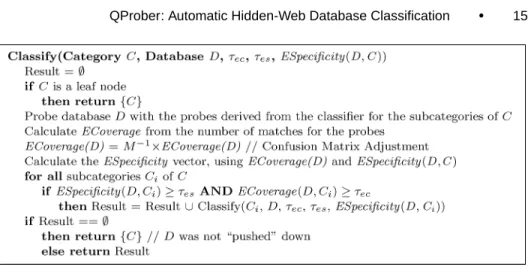
Hence, during the classification of a database D, we multiply M−1 by
Fig. 4. Algorithm for classifying a databaseDinto the category subtree rooted at categoryC.
approximation of the actualCoverage(D) vector. We refer to this adjustment
technique asConfusion Matrix AdjustmentorCMAfor short.
3.5 Using Probing Results for Classification
So far we have seen how to accurately approximate the document category distribution in a database. We now describe a probing strategy to classify a database using these results.
We classify databases in a top-to-bottom way. Each database is first classified by the root-level classifier and is then recursively “pushed down” to the
lower-level classifiers. A database D is pushed down to the categoryCj when both
ESpecificity(D,Cj) andECoverage(D,Cj) are no less than both thresholdτes(for specificity) andτec(for coverage), respectively. These thresholds will typically be equal to theτsandτcthresholds used for theIdealclassification. The final set of categories into which we classifyDis theapproximate classification of D in C.
Definition 3.10. Consider a classification scheme C with categories
C1,. . .,Cn and a database D. If ESpecificity(D) and ECoverage(D) are the approximations of the idealSpecificity(D) andCoverage(D) vectors, respectively, theapproximate classification of D in Cis the setApproximate(D) of categories
Ci that satisfy the following conditions. —ESpecificity(D,Ci)≥τes,
—ESpecificity(D,Cj)≥τesfor all ancestorsCj ofCi, —ECoverage(D,Ci)≥τec,
—ECoverage(D,Cj)≥τecfor all ancestorsCj ofCi, and
—ECoverage(D,Ck)< τecorESpecificity(D,Ck)< τesfor each of the childrenCk ofCi,
where 0≤τes≤1 andτec≥1 are given thresholds.
The algorithm that computes this set is presented in Figure 4. To classify a database Din a hierarchical classification scheme, we callClassify(“root”,D,
Fig. 5. Classifying the ACM Digital Library database.
Example 3.11. Figure 5 shows how we categorized the ACM Digital
Library database. Each node is annotated with the ECoverage and
ESpeci-ficity estimates determined from query probes. The subset of the hierarchy
that we explored with these probes depends on the τes and τec thresholds of choice, which for this case wereτes =0.5 andτec =100. For example, the sub-tree rooted at node “Science” was not explored, because theESpecificityof this node, 0.042, is less than τes. Intuitively, although we estimated that around 430 documents in the collection are generally about “Science,” this was not
the focus of the database and hence the low ESpecificity value. In contrast,
the “Computers” subtree was further explored because of its high ECoverage
(9919) andESpecificity(0.95), but not beyond its children, since their ESpeci-ficityvalues are less thanτes. Hence the database is classified inApproximate=
{“Computers”}.
A potential problem with this algorithm is that a correct classification deci-sion depends on correct classifications in all the nodes that are on the path from the root node to the correct category node(s). Any error made along the path to the correct node is unrecoverable. An alternative approach is to probe the database using the classifiers of all the nodes in the classifica-tion scheme and then decide on the classificaclassifica-tion based on the overall re-sults. However, this approach would require a much larger number of query probes and would considerably increase the cost of our method. Previous work
in hierarchical documentclassification [Sahami 1998] has outlined other
ap-proaches to address this problem, but a full discussion of such extensions is beyond the scope of this article. We simply note here that the techniques used in the case of hierarchical document classification can be adapted for use in the case of hierarchical database classification that we address in this work.
4. EXPERIMENTAL SETTING
We now describe the data (Section 4.1), techniques we compare (Section 4.2), and metrics (Section 4.3) for our experimental evaluation.
4.1 Data Collections
To evaluate our classification techniques, we first define a comprehensive clas-sification scheme (Section 2.1) and then build text classifiers using a set of preclassified documents. We also specify the databases over which we tuned and tested our probing techniques.
Rather than defining our own classification scheme arbitrarily from scratch we instead rely on that of existing directories. More specifically, for our ex-periments we picked the five largest top-level categories from Yahoo!, which were also present in InvisibleWeb. These categories are “Arts,” “Computers,” “Health,” “Science,” and “Sports.” We then expanded these categories up to two more levels by selecting the four largest Yahoo! subcategories also listed in InvisibleWeb. (InvisibleWeb largely agrees with Yahoo! on the top-level cate-gories in their classification scheme.) The resulting three-level classification scheme consists of 72 categories, 54 of which are leaf nodes in the hierarchy. A small fraction of the classification scheme is shown in Figure 5.
To train a document classifier over our hierarchical classification scheme we used postings from newsgroups that we judged relevant to our various
leaf-level categories. For example, the newsgroupscomp.lang.candcomp.lang.c++
were considered relevant to category “C/C++.” We collected 500,000 articles from April through May 2000. 54,000 out of the 500,000 articles, 1000 per leaf category, were used to train the document classifiers, and 27,000 articles were set aside as a development collection for the classifier (500 articles per leaf category). The training set included 381 duplicate articles and 105 of them were crossposted to multiple newsgroups in our dataset. We removed all headers from the newsgroup articles, with the exception of the “Subject” line; we also removed the email addresses contained in the articles. Except for these modifications, we made no other changes to the collected documents. We used the remaining 419,000 articles to build controlled databases as we report below.
To evaluate database classification strategies we used two kinds of databases: “Controlled” databases that we assembled locally and that allowed us to per-form a variety of sophisticated studies, and real “Web” databases.
Controlled Database Set. We assembled 500 databases using the 419,000
newsgroup articles not used in training the classifier. Duplicates accounted for 7246 articles. As before, we assume that each article was labeled with one category from our classification scheme, according to the newsgroup where it
originated. Thus an article from newsgroups comp.lang.c or comp.lang.c++
was regarded as relevant to category “C/C++,” since these newsgroups were
assigned to category “C/C++.” The size of the 500Controlleddatabases that we created ranged from 25 to 25,000 documents. Out of the 500 databases, 350 were “homogeneous,” with documents from a single category, and the remaining 150 were “heterogeneous,” with a variety of category mixes. We define a database as
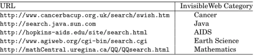
Table I. Some of the Real Web Databases in theWebSet
URL InvisibleWeb Category
http://www.cancerbacup.org.uk/search/swish.htm Cancer
http://search.java.sun.com Java
http://hopkins-aids.edu/site/search.html AIDS http://www.agiweb.org/cgi-bin/search.cgi Earth Science http://mathCentral.uregina.ca/QQ/QQsearch.html Mathematics
“homogeneous” when it has articles from only one node, regardless of whether this node is a leaf node. If it is not a leaf node, then it has an equal number of articles from each leaf node in its subtree. The “heterogeneous” databases, on the other hand, have documents from different categories that reside in the same level in the hierarchy (not necessarily siblings), with different mixture percentages. We believe that these databases model real-world searchable Web databases, with a variety of sizes and foci. These databases were indexed and queried by a SMART-based program [Salton and McGill 1997] supporting both Boolean and vector-space retrieval models.
Web Database Set. We also evaluate our techniques on real Web-accessible
databases over which we do not have any control. We picked the first five databases listed in the InvisibleWeb directory under each node in our clas-sification scheme (recall that our clasclas-sification scheme is a portion of Invis-ibleWeb). This resulted in 130 real Web databases. (Some of the lower-level nodes in the classification scheme have fewer than five databases assigned to them.) Articles that are “newsgroup style” discussions similar to the databases in theControlledset can be found in 12 out of the 130 databases; the other 118 databases have articles of various styles, ranging from research papers to film
reviews. For each database in theWeb set, we constructed a simple wrapper
to send a query and get back the number of matches for each query, which is the only information that our database classification procedure requires. From the initially selected databases, very few (about 5) did not return the number
of matches for the submitted queries. Since QProberneeds these numbers to
classify the databases, we decided not to include these databases in theWebset. The database wrappers were manually configured to send conjunctive queries to each Web database in the proper format. (For example, some databases re-quire the use of the+sign in front of the keywords, whereas others require the use of the “AND” operator.) Also, whenever possible, we configured the wrap-pers with the appropriate settings so that the full underlying databases (rather than, say, a topically focused fraction) are searched. Table I lists five example
databases from theWebset.
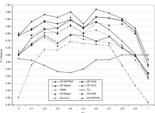
4.2 Techniques for Comparison
We tested variations of our classification technique, which we refer to as
“QProber,” against two alternative strategies. The first one is an
adapta-tion of the technique described in Callan et al. [1999], which we refer to as
“Document Sampling.” The second one is a method described in Wang et al.
[2000] that was specifically designed for database classification. We refer to this method as “Title-Based Querying.” The methods are described in detail below.
4.2.1 QProber. This is our technique, described in Section 3, which uses a document classifier for each internal node of our hierarchical classification scheme. Several parameters and options were involved in the training of the document classifiers. For feature selection, we started by eliminating from con-sideration any word in a list of 400 very frequent words (e.g., “a”, “the”) from the SMART [Salton and McGill 1997] information retrieval system. We then further eliminated all infrequent words that appeared in fewer than three documents. We treated the root node of the classification scheme as a special case, since it covers a much broader spectrum of documents. For this node, we eliminated words that appeared in fewer than five documents. Also, we considered applying the information-theoretic feature selection algorithm from Koller and Sahami [1997, 1996]. We studied the performance of our system without this feature se-lection step (FS=off) and with this step, in which we kept only the top 10% most discriminating words (FS=on). We also experimented with different kinds of classifiers. We created rule-based classifiers using RIPPER [Cohen 1996], as well as using C4.5RULES to extract rules from decision trees generated by
C4.5 [Quinlan 1992]. We refer to these two versions ofQProberasQP-RIPPER
and QP-C4.5, respectively. In addition, we used our technique described in Section 3.3 to derive classification rules from Naive Bayes classifiers [Duda and Hart 1973] and Support Vector Machines with linear kernels [Joachims 1998]. We refer to these versions asQP-BayesandQP-SVM, respectively. After setting up the system, the main parameters that can be varied in our database classification technique are thresholds τec (for coverage) and τes (for speci-ficity). Different values for these thresholds result in different approximations,
Approximate(D), of the ideal classification,Ideal(D).
4.2.2 Document Sampling (DS). Callan et al. [Callan et al. 1999; Callan
and Connell 2001] use query probing to automatically construct a “language model” of a text database (i.e., to extract the vocabulary and associated word-frequency statistics). Queries are sent to the database to retrieve a representa-tive random document sample. The documents retrieved are analyzed to extract the words that appear in them. Although this technique was not designed for database classification, we decided to adapt it to our task as follows.
1. Pick a random word from a dictionary and send a one-word query to the database in question.
2. Retrieve the top-N documents returned by the database for the query.
3. Extract the words from each document and update the list and frequency of words accordingly.
4. If a termination condition is met, go to Step 5; else go to Step 1.
5. Use a modification of the algorithm in Figure 4 that classifies the documents in the sample document collection rather than probing the database itself with the classification rules.
For Step 1, we used a random word from the approximately 100,000 words
in our newsgroup collection. For Step 2, we used N = 4, which is the value
Step 4 we used both the termination conditions described in Callan and Connell [2001] and in Callan et al. [1999]. In Callan and Connell [2001] the algorithm terminates after the retrieval of 500 documents, and in Callan et al. [1999] the algorithm terminates when the vocabulary and frequency statistics asso-ciated with the sample document collection converge to a reasonably stable
state. We refer to the version of the Document Samplingtechnique described
in Callan et al. [1999] as DS99, and we refer to the newer version described in Callan and Connell [2001] simply as DS. After the construction of the lo-cal document sample, the adapted technique can proceed almost identilo-cally as in Section 3.5 by classifying the locally stored document sample rather than
the original database. In our experiments usingDocument Samplingand
lin-ear classifiers, we used the originally generated linlin-ear classifiers and not the rule-based approximations, since the documents in this case are available lo-cally and there is no need to approximate the existing classifiers with rule sets.
The variations ofDocument Samplingthat use different classifiers are named
DS-RIPPER, DS-C4.5, DS-Bayes, and DS-SVM, depending on the classifier
used. We also tested theDS99technique with different classifiers; the results,
however, were consistently worse compared to those for the newer DS
tech-nique. For brevity, in Section 5 we only report the results obtained for DS99
with the RIPPER document classifier. A crucial difference between the
Docu-ment Samplingtechnique andQProberis thatQProberonly uses the number of
matches reported by each database, whereas theDocument Samplingtechnique
requires retrieving and analyzing the actual documents from the database. 4.2.3 Title-Based Querying (TQ). Wang et al. [2001] present three different techniques for the classification of searchable Web databases. For our experi-mental evaluation we picked the method they deemed best. Their technique creates one long query for each category using the title of the category itself (e.g., “Baseball”) augmented by the titles of all of its subcategories. For
exam-ple, the query for category “Baseball” is “baseball mlb teams minor leagues
stadiums statistics college university. . ..” The query for each category is sent to the database in question, the top-ranked results are retrieved, and the average similarity [Salton and McGill 1997] of these documents and the query defines the similarity of thedatabasewith the category. The database is then classified into the categories that are most similar to it. A significant problem with this approach is the fact that a large number of Web-based databases will prune the query if it exceeds a specific length. For example, Google8truncates any query with more than 10 words. The results returned from the database in such cases will not be the expected ones with respect to all the original query terms. The details of the algorithm are described below.
1. For each categoryCi:
(a) Create an associated “concept query,” which is simply the title of the category augmented with the titles of its subcategories;
(b) Send the “concept query” to the database in question; 8http://www.google.com.
(c) Retrieve the top-N documents returned by the database for this query;
(d) Calculate the similarity of these N documents with the query. The
av-erage similarity will be the similarity of the database to categoryCi; 2. Rank the categories in order of decreasing similarity to the database; 3. Assign the database to the top-K ranked categories from the hierarchy. To create the concept queries of Step 1, we augmented our hierarchy with an extra level of “titles,” as described in Wang et al. [2000] . For Step 1(c) we used
the value N =10, as recommended by the authors. We used the cosine
simi-larity function withtf.idf weighting [Salton and Buckley 1988]. Unfortunately,
the value of K in Step 3 is left as an open parameter in Wang et al. [2000].
We decided to favor this technique in our experiments by “revealing” to it the correct number of categories into which each database should be classified. Of course this information would not be available in a real setting, and was not
provided toQProberor theDocument Samplingtechnique.
4.3 Evaluation Metrics
We evaluated classification algorithms by comparing the approximate
clas-sification Approximate(D) that they produce against the ideal
classifica-tion Ideal(D). We could have just reported the fraction of the categories in
Approximate(D) that were correct (i.e., that also appeared inIdeal(D)). However, this would not have captured the nuances of hierarchical classification. For ex-ample, we may have classified a database in the category “Sports,” whereas it is a database about “Basketball.” The metric above would consider this classifica-tion as absolutely wrong, which is not appropriate since, after all, “Basketball” is a subcategory of “Sports.” With this in mind, we adapted theprecisionand
recallmetrics from information retrieval [Cleverdon and Mills 1963]. We first introduce an auxiliary definition. Given a set of categories N, we “expand” it by including all the subcategories of the categories inN, in essence, taking the downward closure of the set of categoriesN in the classification hierarchyC. ThusExpanded(N)= {c∈ C|c∈ N or cis in a subtree of somen ∈ N}. Now we can defineprecisionandrecallas follows.
Definition 4.1. Consider a database Dthat is classified into the set of cat-egoriesIdeal(D), and an approximation ofIdeal(D) given in Approximate(D).
LetCorrect=Expanded(Ideal(D)) andClassified=Expanded(Approximate(D)). Then theprecisionandrecallof the approximate classification ofDare:
precision = |Correct∩Classified| |Classified| recall = |Correct∩Classified|
|Correct| .
To condense precision and recall into one number, we use the F1
-measure [van Rijsbergen 1979],
F1 =
2·precision·recall precision+recall ,
which is only high when both precision and recall are high, and is low for design options that trivially obtain high precision by sacrificing recall or vice versa.
Example 4.2. Consider the classification scheme in Figure 5. Suppose that the ideal classification for a database DisIdeal(D)= {“Programming”}. Then theCorrectset of categories includes “Programming” and all its subcategories, namely, “C/C++,” “Perl,” “Java,” and “Visual Basic.” If we approximateIdeal(D) asApproximate(D)= {“Java”}using the algorithm in Figure 4, then we do not manage to capture all categories in Correct. In fact we miss four out of five such categories and hence recall= 0.2 for this database and approximation. However, the only category in our approximation, “Java,” is a correct one, and
hence precision=1. The F1-measure summarizesrecall andprecisionin one
number,F1=(2·1·0.2)/(1+0.2)=0.33.
An important property of classification strategies over the Web is scalability. We measure the efficiency of the various techniques that we compare by model-ing their cost. More specifically, the maincostwe quantify is the number of “in-teractions” required with the database to be classified, where each interaction is either a query submission (needed for all three techniques) or the retrieval
of a database document (needed only forDocument SamplingandTitle-Based
Querying). Of course, we could include other costs in the comparison (namely, the cost of parsing the results and processing them), but we believe that they would not affect our conclusions, since these costs are CPU-based and are small compared to the cost of interacting with the databases over the Internet.
All methods parse the query result pages to get the information they need. Our method requires very simple parsing, namely, just getting the number of matches from a line of the result. The other two methods require a more ex-pensive analysis to identify the actual documents in the result. To simplify our analysis, we disregard the cost of result parsing, since considering this cost would only benefit our technique in the comparison. In addition, all methods have a local processing cost to analyze the results of the probing phase. This cost is negligible compared to the cost of query submission and document re-trieval. Our method requires the multiplication of the results with the inverse
of the normalized confusion matrices. These arem×mmatrices wherem is
at most the largest number of subcategories for a category in the hierarchical classification scheme. (Recall that we have a small rule-based document clas-sifier for each node in a hierarchical classification scheme.) Sincemwill rarely exceed, say, 15 categories in a reasonable scheme, this cost will be small. The local processing costs forDocument Samplingare similar to our method, except for the fact thatDocument Samplinghas to classify the locally stored collection of sample documents. We also consider this cost negligible relative to other cost components. Finally,Title-Based Queryingrequires calculating the similarities of the documents with the query, and ranking the categories accordingly. Again, we do not consider this cost in our comparative evaluation.
5. EXPERIMENTAL RESULTS
We now report experimental results that we used to tune our system (Section 5.1) and to compare the different classification alternatives both
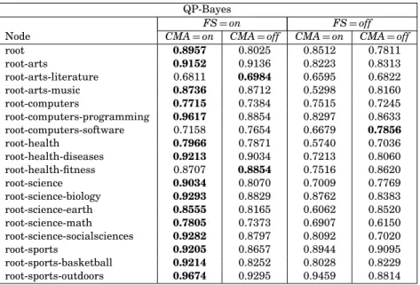
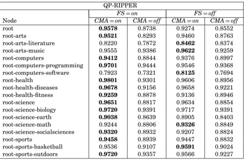
Table II. TheF1-Measure forQP-Bayes, With and Without Feature Selection (FS) and
Confusion-Matrix Adjustment (CMA) QP-Bayes
FS=on FS=off
Node CMA=on CMA=off CMA=on CMA=off
root 0.8957 0.8025 0.8512 0.7811 root-arts 0.9152 0.9136 0.8223 0.8313 root-arts-literature 0.6811 0.6984 0.6595 0.6822 root-arts-music 0.8736 0.8712 0.5298 0.8160 root-computers 0.7715 0.7384 0.7515 0.7245 root-computers-programming 0.9617 0.8854 0.8297 0.8633 root-computers-software 0.7158 0.7654 0.6679 0.7856 root-health 0.7966 0.7871 0.5740 0.7036 root-health-diseases 0.9213 0.9034 0.7213 0.8060 root-health-fitness 0.8707 0.8854 0.7516 0.8620 root-science 0.9034 0.8070 0.7009 0.7769 root-science-biology 0.9293 0.8829 0.8762 0.8383 root-science-earth 0.8555 0.8165 0.6062 0.8520 root-science-math 0.7805 0.7373 0.6907 0.6150 root-science-socialsciences 0.9282 0.8797 0.8092 0.7020 root-sports 0.9205 0.8657 0.8944 0.9095 root-sports-basketball 0.9214 0.8252 0.8028 0.8229 root-sports-outdoors 0.9674 0.9295 0.9459 0.8814
for the Controlled database set (Section 5.2) and for the Web database set
(Section 5.3).
5.1 Tuning QProber and DS
QProberandDShave some open parameters that we tuned experimentally by
using a set of 100Controlleddatabases (Section 4.1). These databases did not participate in any of the subsequent experiments.
We examined whether the information-theoretic feature selection
(Section 4.2) and the confusion matrix adjustment of the probing results (Section 3.4) affected the classification accuracy. We ranQProberwith (FS=on) and without (FS=off) this feature selection step, and with (CMA=on) and
without (CMA=off) the confusion matrix adjustment step, and we evaluated
the classification results of theindividualclassifiers. We did this for our four
versions ofQProber, namely,QP-RIPPER,QP-C4.5,QP-Bayes, andQP-SVM.
Unfortunately, the C4.5 classifier underlying QP-C4.5 could not handle the
training set with all the features, so we could not create the C4.5 classifiers withFS=off. However, it is reported that feature selection helps C4.5 avoid overfitting [Kohavi and John 1997; Koller and Sahami 1996]; hence we believe
that the results without feature selection would have been worse forQP-C4.5
anyway. We performed the same experiment for the five different versions of
DSas well. Since the conclusions from the experiments were similar, in the
following we only report the results for the tuning ofQProber.
For evaluation, we used theF1-measure for theflatset of categories associ-ated with each classifier and for each of the 100 databases that contained doc-uments in the categories in question. We compared the average performance of the classifiers over the training set. Tables II through V report the results for all
Table III. TheF1-Measure forQP-C4.5, With and Without
Confusion Matrix Adjustment (CMA) QP-C4.5
Node CMA=on CMA=off
root 0.9195 0.8509 root-arts 0.9000 0.8693 root-arts-literature 0.7895 0.7774 root-arts-music 0.8755 0.8898 root-computers 0.8620 0.8374 root-computers-programming 0.9226 0.9017 root-computers-software 0.8151 0.8497 root-health 0.8724 0.8580 root-health-diseases 0.9611 0.9374 root-health-fitness 0.7976 0.8251 root-science 0.9322 0.9108 root-science-biology 0.9160 0.9201 root-science-earth 0.5299 0.6198 root-science-math 0.6992 0.6977 root-science-socialsciences 0.9262 0.8898 root-sports 0.9189 0.8864 root-sports-basketball 0.8486 0.8463 root-sports-outdoors 0.8405 0.8510
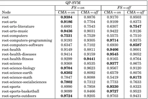
Table IV. TheF1-Measure forQP-SVM, With and Without Feature Selection (FS), and
Confusion Matrix Adjustment (CMA) QP-SVM
FS=on FS=off
Node CMA=on CMA=off CMA=on CMA=off
root 0.9384 0.8876 0.9170 0.8503 root-arts 0.9186 0.7704 0.9109 0.8373 root-arts-literature 0.6891 0.7543 0.6307 0.7547 root-arts-music 0.9436 0.9031 0.9422 0.9126 root-computers 0.7531 0.7529 0.5575 0.7510 root-computers-programming 0.9193 0.9305 0.9714 0.9375 root-computers-software 0.6347 0.7102 0.6930 0.8587 root-health 0.9149 0.8811 0.9406 0.9001 root-health-diseases 0.9414 0.9159 0.9545 0.9052 root-health-fitness 0.9299 0.9441 0.9165 0.8764 root-science 0.9368 0.8535 0.9377 0.8675 root-science-biology 0.9704 0.9623 0.9567 0.9120 root-science-earth 0.8302 0.8092 0.6579 0.8076 root-science-math 0.7847 0.8088 0.5419 0.8173 root-science-socialsciences 0.7802 0.7312 0.7733 0.7633 root-sports 0.8990 0.7958 0.9330 0.8323 root-sports-basketball 0.9099 0.8466 0.9727 0.9523 root-sports-outdoors 0.9724 0.9205 0.9703 0.9431
the nonleaf nodes of our classification scheme; the best results are highlighted in boldface.
The results were conclusive for the confusion matrix adjustment (CMA). For QP-RIPPER, the results were consistently better after the application of
the adjustment. For the otherQProberversions, CMA improved the results in