The ParTriCluster Algorithm for Gene Expression Analysis
Renata Araujo Guilherme Ferreira Gustavo Orair
Wagner Meira Jr. Renato Ferreira Dorgival Guedes
Department of Computer Science Universidade Federal de Minas Gerais
{renata,trielli,orair,meira,renato,dorgival}@dcc.ufmg.br
Mohammed Zaki
Department of Computer Science Rensselaer Polytechnique Institute
[email protected] Abstract
Analyzing gene expression patterns is becoming a highly relevant task in the Bioinformatics area. This analysis makes it possible to determine the behavior patterns of genes under various conditions, a fundamental information for treating diseases, among other applications. A recent advance in this area is the Tricluster algorithm, which is the first algorithm capable of determining 3D clusters (genes x samples x timestamps), that is, groups of genes that behave similarly across samples and timestamps. However, while biological experiments collect an increasing amount of data to be analyzed and correlated, the triclustering problem is NP-Complete, and its parallelization seems to be an essential step towards obtaining feasible solutions. In this work we propose and evaluate the implementation of a parallel version of the Tricluster algorithm using the filter-labeled-stream paradigm supported by the Anthill parallel programming environment. The results show that our parallelization scales well with the data size, being able to handle severe load imbalances that are inherent to the problem. Further, the parallelization strategy is applicable to any depth-first searches.
1 Introduction
Since the start of the Genoma project, Bioinformatics became an important area for the success of this initiative and others that followed. Bioinformatics comprises the use of computational resources for sequencing, comparing, and interpreting the genetic code, which brings information that determines the functions performed by living beings [1]. Among the several problems studied in Bioinformatics, the analysis of gene expression patterns, that is, determining the correlations among genes and the occurrence of phenomena such as diseases across time, is challenging and relevant to the development of novel treatments, among other applications [2].
There have been proposed a large number of strategies for clustering towards the analysis of gene expression data [3, 4]. However, the results from the application of standard clustering strategies are not good enough for analysis, as a consequence of their inability to find correlations among more than one dimension, nominally, genes and samples.
A large number of algorithms that cluster, simultaneously, both genes and samples have been proposed recently - a strategy that is known as biclustering. Formally, biclustering algorithms determine sets of genes and sets of samples where the genes present similar behavior for all selected samples. There are some algorithms and heuris-tics proposed for the biclustering problem, such as SAMBA [5], OP-Clusters [6], and xMOTIFs [7], providing good results.
Besides the determination of biclusters of genes and samples, there is also an increasing interest in mining pat-terns across time [2]. However, all except one of the approaches proposed so far are restricted to two dimensions, finding patterns that correlate the gene and time dimensions, but discarding the sample dimension. The algorithm Tricluster [2] is the first and, as far as we know, the only algorithm that determines gene-expression clusters in three dimensions, that is, genes that express similarly for a given set of samples and time periods.
Although the triclustering technique helps to find better solutions for sake of the analysis of gene expressions, the problem is still NP-Complete [2], as well as biclustering [8] (they may be seen as the problem of determining the maximal clique in a bipartite graph), justifying the need for strategies that reduce their execution time.
The Tricluster algorithm not only subsumes functionally the existing bicluster approaches but it also provides some additional features. In summary, the algorithm is capable of finding significative clusters located arbitrarily and overlapping; mining different types of triclusters that are similar with respect to their absolute, scaled, and shifted values; and putting together or discarding triclusters that contain large overlapping regions, automatically relaxing the similarity criterion, and helping the user to focus on the most relevant clusters.
Thus, the parallelization of the Tricluster algorithm seems to be a solution for making the analysis of large datasets feasible, and it is the starting point of our paper.
2 Related work
Since the Tricluster algorithm has been published recently, we are not aware of any effort towards its paral-lelization. However, it might be relevant to point out some of the algorithms that have been paralelized under the same programming model that we use: the filter-stream paradigm (using the Anthill platform).
The Apriori algorithm is capable of doing association analysis determining association rules, which show at-tribute instances (usually called items) that occur frequently together and present a causality relation between them. The ID3, on the other hand, is a decision tree algorithm, in which the leaf nodes are the individual data ele-ments. The basic idea is to use a top-down and greedy search on the data to find the most discriminating attribute on each level of the tree. And, finally, the K-means algorithm is capable of doing a cluster analysis, partitioning and determining groups of objects that are similar regarding a user-given similarity criteria.
All these three algorithms presented (Apriori [9], ID3 and K-means [10]) were paralelized on the Anthill platform, using the filter-stream paradigm, and presented very good results, scaling almost linearly and even presenting a superlinear speedup in some cases.
3 The algorithm Tricluster
In this section we briefly present the sequential version of Tricluster, as a basis for discussing our parallelization strategy.
LetG={g0, g1, ..., gn−1}be a set ofngenes,S ={s0, s1, ..., sm−1}be a set ofmsamples, (that is, different tissues or experiments), and T = {t0, t1, ..., tl−1}a set of lexperimental timestamps. A database that contains 3D gene expression is a matrixnxmxl,D =GxSxT, where the dimensions are genes, samples, and time, respectively. A triclusterCis a submatrix ofD, whereC =XxY xZ,X ⊆G,Y ⊆S, andZ ⊆T, provided that certain conditions of homogeneity are satisfied.
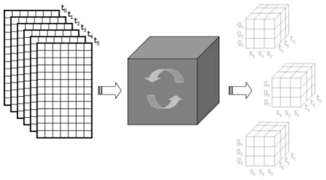
The basic functionality of the Tricluster algorithm is illustrated in Figure 1: it receives as input a set of matrices (one for each time stamp), in which the lines represent the genes and the columns represent the samples, and generates the triclusters as output.
Figure 1. Input and output of the Tricluster algorithm.
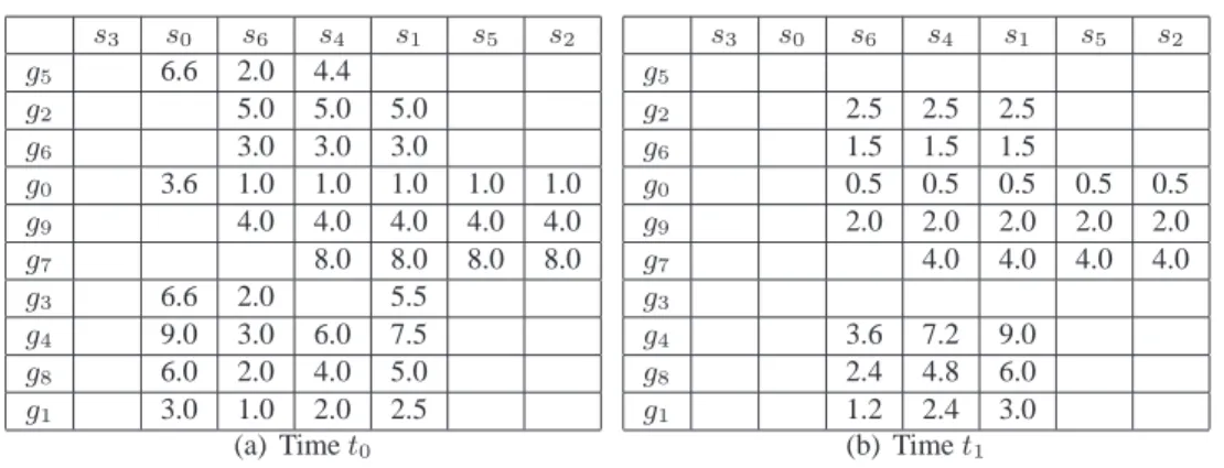
Therefore, this algorithm receives as input the aforementioned 3D database (as illustrated by Figure 2) and a set of parameters: ǫ,mx,my,mz,δx,δy, andδz, which will determine whether a tricluster is valid or not. The numbers in the tables of Figure 2 correspond to gene expression levels (the empty spaces are just to make the visualization easier). The output is the set of maximal valid triclusters from the database. An example of some clusters found by the algorithm may be found in Figure 3.
The Tricluster algorithm may be divided into three main steps:
1. For each matrixGxSassociated with a timestamptand for each pair of samples in those matrixes, we find the valid range intervals for gene expressions, called ratio-ranges. Then, for each timestamp, we build the multigraph from these intervals, called range multigraph.
2. We mine the maximal biclusters from the range multigraph.
3. We build a graph based on the mined biclusters (mapping the time periods as vertices and the valid biclusters as edges), and find the maximal triclusters.
It is also possible to remove or merge triclusters based on an overlap criterion. This is a post-processing step that is not detailed here, since it has not been parallelized yet. In the next subsections, we present the algorithm in detail.
s0 s1 s2 s3 s4 s5 s6 g0 3.6 1.0 1.0 1.0 1.0 1.0 g1 3.0 2.5 2.0 1.0 g2 5.0 5.0 5.0 g3 6.6 5.5 2.0 g4 9.0 7.5 6.0 3.0 g5 6.6 4.4 2.0 g6 3.0 3.0 3.0 g7 8.0 8.0 8.0 8.0 g8 6.0 5.0 4.0 2.0 g9 4.0 4.0 4.0 4.0 4.0 (a) Timet0 s0 s1 s2 s3 s4 s5 s6 g0 0.5 0.5 0.5 0.5 0.5 g1 3.0 2.4 1.2 g2 2.5 2.5 2.5 g3 5.5 2.0 g4 9.0 7.2 3.6 g5 4.4 2.0 g6 1.5 1.5 1.5 g7 4.0 4.0 4.0 4.0 g8 6.0 4.8 2.4 g9 2.0 2.0 2.0 2.0 2.0 (b) Timet1
Figure 2. Gene database for timest0andt1.
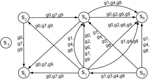
s3 s0 s6 s4 s1 s5 s2 g5 6.6 2.0 4.4 g2 5.0 5.0 5.0 g6 3.0 3.0 3.0 g0 3.6 1.0 1.0 1.0 1.0 1.0 g9 4.0 4.0 4.0 4.0 4.0 g7 8.0 8.0 8.0 8.0 g3 6.6 2.0 5.5 g4 9.0 3.0 6.0 7.5 g8 6.0 2.0 4.0 5.0 g1 3.0 1.0 2.0 2.5 (a) Timet0 s3 s0 s6 s4 s1 s5 s2 g5 g2 2.5 2.5 2.5 g6 1.5 1.5 1.5 g0 0.5 0.5 0.5 0.5 0.5 g9 2.0 2.0 2.0 2.0 2.0 g7 4.0 4.0 4.0 4.0 g3 g4 3.6 7.2 9.0 g8 2.4 4.8 6.0 g1 1.2 2.4 3.0 (b) Timet1
Figure 3. Some clusters for the sample databases
3.1 Building the range multigraph
Before we present the strategy for building the range multigraph, we need to introduce some terminology.
• rab x = dxa dxb
is the ratio of the gene expression values of genegxfrom columnssaandsb, wherex∈[0, n−1],
and it is called ratio value;
• ratio range is the interval of ratio values,[rl, ru], whererl ≤ru;
• Gab([rl, ru]) ={gx :rabx ∈ [rl, ru]}is the set of genes, (gene-set), such that its ratio value from columns saesbare within the given ratio range, and ifrabx <0, all values of the same column are either negative or non-negative.
In the first step, the algorithm Tricluster tries to determine the valid ratio ranges that may help finding a bicluster. Formally, a ratio range is valid if:
• maxmin(|(|ruru||,,||rlrl|)|)−1≤ǫ, whereǫis a maximal pre-defined ratio value threshold.
• ifrab
x <0, all values dxadxb in the same column have the same signal (negative or non-negative).
• [rl, ru]is maximal, that is, it is not possible to add another gene toGab([rl, ru])and still satisfy the current ǫ.
Intuitively, the algorithm looks for the maximal ratio ranges that are withinǫand contain at leastmxgenes. Notice that there may be multiple intervals (ratio ranges), between two columns and some of the genes may not belong to any interval.
Figure 4 illustrates the ratio values for various genes using columnss0/s6 at timet0 for the database example given in Figure 2. Givenǫ= 0.01 andmx= 3, there is just one valid ratio range, [3.0,3.0], which is associated with the gene-setGs0,s6([3.0,3.0]) ={g1, g4, g8}.
0 6
ROW g g g g g g1 4 8 3 5 0 S /S 3.0 3.0 3.0 3.3 3.3 3.6
Figure 4. Ratio values from the columnss0/s6at timet0from Figure 2
Given the set of all valid ratio ranges across any pair of columns sa e sb, a < b, given as Rab = {Rab
i =
[rab
li, ruiab] :sa, sb ∈S}, we build a directed range multigraph,M = (V, E), whereV =S(set of all samples), and for eachRab
i ∈ Rabthere is a directed edge(sa, sb)∈E. Further, each edge in the range multigraph is associated with a gene-set corresponding to the range on that edge.
For instance, assume thatmx= 3andǫ= 0.01. Figure 5 shows the range multigraph built from the database given in Figure 2, for timestampt0. In this case, for example, there are two edges from samples1to samples6. It indicates that two valid ratio ranges were found for this pair of samples, one consisted of genes{g0, g2, g6, g9} and the other consisted of genes{g1, g4, g8}. Notice that there may be a different multigraph for timestampt1.
3.2 Mining biclusters
The range multigraph is a compact representation of all valid ratio ranges that may be used to mine potential biclusters for each timestamp, discarding all irrelevant data.
The algorithm Bicluster performs a depth-first search in the range multigraph for mining all biclusters, as shown in the pseudo-code in Algorithm 1. The input to the algorithm is a set of parameters: ǫ,mx,my,δx,δy, the multigraphMtfor a timestampt, and a set of genesGand samplesS. This algorithm generates as output the final set of all biclustersCtfor that timestampt.
Bicluster is a recursive algorithm that takes, for each call, a candidate bicluster,C=XxY, and a set of non-processed samplesP. The parameters for the initial call are a clusterC=Gx∅, containing all genesG, but no samples, and P = S, since all samples should be processed. BeforeCis given as a parameter for the recursive call, we ensure that |C.X| ≥ mx(it is obviously true for the initial call and also for line 15 of the algorithm). Line 2 verifies whether the cluster is within the gene and sample thresholds given byδx,δy, and also the minimum number of samplesmy. If both conditions are fulfilled, it verifies whetherC is not already a subset of a maximal clusterC′. If it is not a subset,Cis added to theCt(line 5) and any clusterC′′∈ C that is already inCis deleted (line 4).
Lines 7-17 generate a new candidate cluster by extending the current candidate with another sample. They also build the proper gene-set for the new candidate, before making a recursive call. Bicluster starts by adding to cluster C, each of the new samplessb ∈P (line 6), for determining the new candidateCnew(lines 7-8). Samples that have been already considered are removed fromP (line 9). Letsabe all samples added toCbefore the last recursive
Figure 5. Directed Range multigraph
call. If there is no such vertexsa(as it occurs in the initial call), the algorithm just call Bicluster informing a new candidate. Otherwise, Bicluster tries all possible combinations for each edge that has a valid intervalRab
i between saandsbfor allsa∈C.Y (line 13), determining their intersection which is the gene-set,Tallsa∈C.Y G(Rabi ), and verifies the intersection withC.Xto determine the valid genes of the new clusterCnew(line 14). If the new cluster has at leastmxgenes, then another recursive call to Bicluster is performed (lines 15-16).
Time # (genes) × (samples)
t0 C1 (g1g4g8) × (s0s1s4s6) t0 C2 (g0g2g6g9) × (s1s4s6) t0 C3 (g0g7g9) × (s1s2s4s5) t1 C1 (g1g4g8) × (s0s1s4s6) t1 C2 (g0g2g6g9) × (s1s4s6) t1 C3 (g0g7g9) × (s1s2s4s5) t3 C1 (g1g6g8) × (s0s4s5) t3 C2 (g0g7g9) × (s1s2s4s5) t8 C1 (g1g4g8) × (s0s1s4) t8 C2 (g2g6g9) × (s1s4s6)
Figure 6. Triclusters for the sample database
For instance, consider how the clusters are mined in the range multigraphMt0 shown in Figure 4. Letmx= 3,
my = 3, andǫ= 0,01. Initially, Bicluster starts from vertexs0, and candidate cluster{g0, ..., g9}x{s0}. Next, the vertexs1is processed. Since there is just one edge, the new candidate is{g1, g3, g4, g8}x{s0, s1}. After pro-cessings1, we considers4and two edges are taken into account: (i) for the edge associated withG={g1, g4, g8}, the new candidate is {g1, g4, g8} x{s0, s1, s4}and is considered valid, (ii) for the other edge, associated with G={g0, g2, g6, g7, g9}, however, the number of genes is below the thresholdmx, and the candidate is discarded. s6is processed next. Among the two edges betweens4es6, just one will generate a candidate cluster{g1, g4, g8} x {s0, s1, s4, s6}. Since this cluster is maximal and fulfill all parameter-related requirements, it becomes one (C1) of the maximal triclusters shown in Figure 6. The process explained here is illustrated in Figure 7.
Simi-Bicluster (C=XxY,P): ifCsatisfiesδx,δythen 1 if|C.Y| ≥mythen 2 if∀C′ ∈ Ct |C⊂C′ then 3 Delete anyC′′ ∈ C, ifC′′ ⊂C; 4 Ct ←− Ct+C ; 5 foreachsb∈Pdo 6 Cnew←−C; 7 Cnew.Y ←−Cnew.Y +s b; 8 P ←−P−sb; 9 ifC.Y =∅then 10 Bicluster(Cnew,P); 11 else 12
forallsa∈C.Y and eachRabi ∈ Rab|G(Rabi )
T C.X| ≥mxdo 13 Cnew.X←−(T allsa∈C.YG (Rab i )) T C.X; 14 if|Cnew.X| ≥mx then 15 Bicluster(Cnew,P) 16 Algorithm 1: Bicluster
larly, when the process starts from s1, we will find two other clusters: C3 = {g0, g7, g9}x {s1, s2, s4, s5} and C2 = {g0, g2, g6, g9} x {s1, s4, s6}. The intuition here is that the algorithm looks for maximal cliques in the sample, such that they have at leastmyvertices and also at leastmxgenes.
3.3 Mining triclusters
After we find the maximal biclusters Ctfor each timestamp, we use them to mine the maximal triclusters by enumerating the subsets for each timestamp, as shown in Algorithm 2. We employ a strategy that is similar to the clique mining of the Bicluster algorithm (Algorithm 1).
Tricluster (C=XxY xZ,P): ifCsatisfiesδx,δy,δzthen 1 if|C.Z| ≥mzthen 2 if∀C′ ∈ C|C⊂C′ then 3 Delete anyC′′ ∈ C, ifC′′ ⊂C; 4 C ←− C+C; 5 foreachtb∈Pdo 6 Cnew.Z←−C.Z+t b; 7 P ←−P−tb; 8
forallta∈C.Zand each biclusterctia∈ Cta
satisfying|cta i .X T C.X| ≥mxand|cta i .Y T C.Y| ≥mydo 9 Cnew.X←−(T allta∈C.Z cta i .X) T C.X; 10 Cnew.Y ←−(T allta∈C.Zc ta i .Y) T C.Y ; 11 if|Cnew.X| ≥mx and|Cnew.Y| ≥my
and the ratios at timetb,taare coherent then 12
Tricluster(Cnew,P)
13
Algorithm 2: Tricluster
For instance, from Figure 2, it is possible to determine the biclusters associated with timestamps t0 e t1, as shown in Figure 6. Since the clusters are the same, we calculate the biclusters for the timestampst3 andt8 (the database is not provided for space restrictions) for illustrating the Tricluster algorithm.
Figure 7. Depht-first search to mine the potencial biclusters.
Assume that the minimum size is mx x my x mz = 3 x 3 x 3. Tricluster starts from timestamp t0, which contains three biclusters. Consider the cluster C1 att0, denoted asC1t0. For each biclusterCt1, justCt
1
1 may be used for extending sinceCt0
1 TCt
1
1 ={g1, g4, g8}x{s0, s1, s4, s6}, satisfying the input parameters. We continue by checking the biclusters from timestampt3, but the cluster cannot be extended in this case. Finally, we verify whether the cluster may be extended throughCt8. The final result is{g
1, g4, g8}x{s0, s1, s4}x{t0, t1, t8}. We also try all other possible paths, maintaining just the maximal triclusters.
3.4 Algorithm analysis
Since it is necessary to evaluate all pairs of samples to compute all ratios and to find all valid intervals for all genes, building the range multigraph isO(|G||S|2|T|).
Mining biclusters and triclusters is equivalent to enumerate the conditional maximal cliques (that is, cliques that satisfy the parameters (mx, my, mz, δx, δy, and δz) from the range multigraph and the bicluster graph, respectively. In the worst case scenario there may be an exponential number of clusters and these two steps are the most expensive. The exact number of mined clusters is a function of the database and input parameters.
However, for reasonable databases of gene expression, the Tricluster algorithm is usually efficient because of the following reasons. First, the range multigraph approach removes noise and irrelevant data. Second, the depth-first search demands few iterations, since the databases usually contain a significantly smaller number of samples and timestamps than genes. Finally, Tricluster maintains sets of intermediary gene sets for all candidate clusters, allowing to prune the search whenever an input parameter is not satisfied. The merge and prune step is applied just on the overlaping clusters, at a cost ofO(|C|log(|C|).
We also profiled the sequential version of the algorithm in order to identify the most time consuming portions of the code. We found that most of the execution time (65%) is associated with the determination of biclusters (30%) and triclusters (35%). Further, most of the execution time for both cases is associated with the depth-first search that will lead to the maximal clusters.
4 The algorithm ParTriCluster
In this section we present ParTriCluster, our parallel version of Tricluster. We start by presenting the Anthill en-vironment, which is used as a basis for the parallelization implemented. Then we describe our proposed algorithm, ParTriCluster, and discuss the parallelization dimensions exploited and its advantages.
4.1 Anthill
Building applications that may efficiently exploit parallelism while maintaining good performance is a chal-lenge. In this scenario, given their size, datasets are usually distributed across several machines in the system to improve access bandwidth. Success in this approach depends on the application being divided into portions that may be instantiated on different nodes of the system for execution. Each of these portions performs part of the transformation on the data starting from the input dataset and proceeding until the resulting dataset is produced, in what is called the filter-stream approach. originally proposed for Active Disks [11] and later extended as a programming model suitable for a Grid environment [12].
In the filter-stream model, filters are the representation of each stage of the computation, where data is formed, and streams are abstractions for communication which allow fixed-size untyped data buffers to be trans-ferred from one filter to the next. Creating an application is a process retrans-ferred to as filter decomposition. In this process, the application is modeled as a dataflow computation and then broken into a network of filters, creating task parallelism as in a pipeline. At execution time, multiple (transparent) copies of each of the filters that compose the application are instantiated on several machines of the system and the streams are connected from sources to destinations.
Our run-time system, Anthill [10] (illustrated in Figure 8), tries to exploit the maximum parallelism in appli-cations structured in the filter-stream model by using three possibilities: task parallelism, data parallelism, and asynchrony. By dividing the computation into multiple pipeline stages (task parallelism), each one replicated mul-tiple times (to handle data in parallel), we can have a very fine-grained parallelism and, since all this is happening asynchronously, the execution is mostly bottleneck free. In order to reduce latency, the grain of the parallelism should be defined by the application designer at run-time.
In our experience, we observed that when we decomposed our data intensive applications into filters, the natural solution was often a cyclic graph, where the execution consisted of multiple iterations over the filters. An applica-tion would start with data representing an initial set of possible soluapplica-tions and as those passed down the filters new candidate solutions would be created. Those, in turn, would have to be passed through the network to be processed themselves. Also, we noticed that this behavior led to asynchronous executions, in the sense that several solutions (possibly from different iterations) might be tested simultaneously at run-time.
One important characteristic separates the Anthill environment from its predecessors: given the cyclic nature of the computation, there are often dependencies among different data that flow through the cycle. Since each stage of computation may have multiple replicas, we must have a way to state that the result of a computation in a given cycle be fed back to a specific instance of another stage. That may be necessary because, for example, there may be some state associated with all inter-dependent pieces of data and that can reside in only one filter instance, so all dependent data must be routed through that specific instance. The abstraction for that in the Anthill is called a labeled stream. It is created by allowing the programmer to associate a label with each message and a mapping function (hash) that associates each possible label with a specific filter instance.
This mechanism gives the application total control over the routing of its messages. Because the hash function is called at runtime, the actual routing decision is taken individually for each message and can change dynamically as the execution progresses. This feature conveniently allows dynamic reconfiguration, which is particularly useful to balance the load on dynamic and irregular applications. The hash function may also be slightly relaxed, in the sense that its output does not have to be one single instance. Instead, it can output a list of those. In that case, a
Figure 8. The Anthill platform.
message can be replicated (multicast) or even broadcast. This is particularly useful for applications in which one single input data element influences several output data elements.
4.2 Parallelization strategy
In this section we present the parallelization strategy employed. The basic principle of the Tricluster algorithm is that it consists of two depth-first searches. The first search finds maximal biclusters for each timestamp in the database and the second search finds maximal triclusters. Biclusters are determined by traversing a multigraph that relates pairs of samples in terms of the sets of genes that present similar behavior in both samples. The basic procedure here is to determine the maximal path in the graph where the same set of genes occurs. Triclusters are determined by traversing a similar multigraph that relates pairs of timestamps in terms of the sets of biclusters that occurr in both timestamps. Again, the basic procedure is to determine the maximal path in the graph where the same set of biclusters occurs. For both biclusters and triclusters, the process starts by building the proper multigraph and then by traversing it. Notice that the second multigraph is built using the biclusters extracted from the first multigraph.
There are four basic entities involved here: the database, the gene multigraph, the biclusters and their multi-graph, and the triclusters. Our parallelization strategy is based on these four entities and their distribution, imple-menting data parallelism for each entity. We defined four filters that are described in the remaining of this section, each of them handling an entity. Figure 9 presents the scheme of filters and their relationships.
The first filter, called the Ratio filter, is responsible for calculating the ratio values for pairs of samples, infor-mation that is necessary for building the range multigraph. One of the challenges of this parallelization is the size of the database. Thus, we have to partition it so that it is still possible to calculate those ratio values, and the best strategy is to partition in the gene dimension, where each instance of the filter is responsible for a set of genes and is capable of calculating the ratio values for each gene for all pairs of sample. These values are sent through a
Figure 9. The scheme of filters.
labeled stream to the second filter, using the identifier of the samples (that is, the sample pair) from the ratio as label. The pseudo-code of the Ratio filter can be seen in Algorithm 3.
Ratio Filter :
fori=my rank;i < number of timestamps;i=i+Reader instancesdo 1
opens the databasedicorresponding to timestampi; 2
foreach linel∈dido 3
foreach pair of samplessxsy(in whichx < y) do 4
determines the ratio value for genegl; 5
sends this value to the corresponding instance of the Edge filter;
6
Algorithm 3: Pseudo-code of Ratio Filter
The second filter is responsible for determining whether the potential edges of the range multigraph are valid or not for sake of determining a bicluster, being called the Edge filter. We present a pseudo-code for this filter in Algorithm 4.
As mentioned, each instanceEi of this filter receives the ratio values that are associated with a pair of samples for all genes (line 1). It’s important to remember that each instance may be responsible for more than one pair of samples in the case that the number of instances is less than the number of sample pairs. For each pair of samples that the instance is responsible for, it also determines the valid intervals, that is, the ratio ranges (line 3). Thus, each instance is responsible for the edges between the pair of samples that it is responsible for. Notice that after all instances of the edge filter analyze all ratio values, the range multigraph is ready, but spread across the various instances. We then need to find the biclusters by traversing this multigraph, as described next.
Each instance Ei of the second filter initiates the search process by sending the information of their initial potential biclusters (that is, the genes found in the valid ratio ranges, and the two samples that corresponds to the pair of samples in which this valid range was found) to the other instances (line 4). Thus, if a filter instance is responsible for a valid edge ofsasb, it sends the gene-set of this edge with the samplessaandsbto all instances that are responsible for the edges of sbsc, wheresc represents all remaining samples greater thansb. For short,
we will use the terminology extending a path for denoting successful searches. Therefore, whenever an instance receives such information (line 6), it verifies whether it is possible to extend it using the edges that it is responsible for (lines 8-12). To do that, the instances calculate the intersection of the genes of the potential bicluster received with the genes of the valid ranges that it has (line 8). When it is possible to extend this path, that is, the number of genes in the intersection bicluster is greater than the minimum number of genes (mx), it includes in the intersection bicluster the samples from the potential bicluster received added with sample sc (line 10) and sends it to all the instances that are responsible for a pair of samples scsd, in which sd are all the samples remaining greater then sc. Besides, it also checks whether the intersection bicluster is already a valid bicluster (checking the minimum number of samplesmy) and, in case it is, the instance sends this bicluster to the instance of the third filter, Bicluster, that is resposible for the timestamp that bicluster corresponds to.
Edge Filter :
receives the ratio values of all genes for the pair of samplessasb∈Ei(in whicha < b); 1
foreachsasb∈Eido 2
calculates all the valid ratio ranges (edges betweensasb); 3
sends the initial potencial biclusters to theEj|sbsc∈Ej(in whichb < c); 4
repeat 5
receives a message with a potencial bicluster (along with the information that it came from a pairsasb); 6
foreachsbsc∈Eido 7
calculates the instersection of the genes of the potencial bicluster with the genes of each valid range of this sample pair;
8
if the number of genes of the bicluster resulted from the intersection≥mx then
9
puts in the intersection bicluter the samples from potential bicluster received added with samplesc; 10
sends the intersection bicluster toEj|scsd∈Ej, (in whichc < d); 11
if the number of samples of the bicluster resulted from the intersection≥my then
12
sends the intersection bicluster to the Bicluster instances that are responsible for the timestamp that the
13
intersection bicluster belongs to;
until there are no more messages to be received ; 14
Algorithm 4: Pseudo-code of Edge Filter
We will use the multigraph of Figure 5 to give an example of this process. Each instance of the Edge filter starts with all genes. When it is determined that the instance responsible for the edges of s0s1 contains an edge labeled with genesg1, g3, g4, g8, this instance sends this information for all instances that are responsible for the pair of samples s1sx, wherex > 1. The instance that takes care of the edges of s1s4, for example, receives the information that there is a valid path from s0 tos1, and tries to extend it by adding the edges of s1s4. More specifically, it calculates the intersection between the gene sets of the path and each potential edge so that it may determine whether the path is still valid. In our example, it finds that it is valid for one of the edges ofs1s4 (the edge associated with genesg1, g4, g8) and not for the other (the edge associated with genesg0, g2, g7, g9) because the number of genes is smaller thanmx. Thus, the path becomess0s1s4. The same instance then sends this path to all instances that are responsible for the edges s4sx, wherex > 4. One instance that receives such path is the one responsible for the edges of s4s6, where the edge associated with the genes g1, g4, g8 is also added to the path. The potential bicluster represented by this path is sent to the third filter, Bicluster. Notice that the Edge filter is responsible for generating all possible paths, enumerating all potential biclusters, which are verified by the Bicluster filter, as described next. Further, this enumeration is performed in parallel exploiting the maximum number of parallelization opportunities inherent to the graph being searched.
One point that we did not discuss in detail is that the biclusters are determined for each timestamp. In practice, this timestamp is also part of all messages, but it is only used for addressing in the filters Bicluster and Tricluster. For instance, when we mentioned the labels0s1, it wass0s1, t0. Each Bicluster filter instance is responsible for all biclusters associated with a pair of timestamps, that is, an edge in the graph of biclusters. We present the pseudo-code for filter Bicluster in Algorithm 5. The Edge filter performs a selective multicast of potential biclusters so
Bicluster Filter :
receives all the bicluster corresponding to timestampti|ti∈Bi; 1
foreachtatb∈Bido 2
calculates the valid biclusters making the instersections between the valid biclusters of timestamptaand timestamptb, in which 3
b > a;
sends the initial potencial triclusters to the Bicluster instancesBj|tbtc∈Bj; 4
repeat 5
receives a message with a potencial tricluster (along with the information that it came from a pairtatb); 6
foreachtbtc∈Bido 7
calculates the instersection of the genes and samples of the potencial tricluster with the genes and samples of each valid
8
bicluster of this pair of timestamps;
if the number of genes of the tricluster resulted from the intersection≥mx and the number of samples of the tricluster
9
resulted from the intersection≥my then
puts in the intersection tricluster the timestamps from the potential tricluster received added with timestamptc; 10
sends the intersection tricluster toBj|tctd∈Bj, (in whichc > d); 11
if the number of timestamps of the tricluster resulted from the intersection≥mz then
12
sends the intersection tricluster to the Tricluster filter;
13
until there are no more messages to be received ; 14
Algorithm 5: Pseudo-code of Bicluster Filter
that each potential bicluster reaches the proper filter instances. The Bicluster filter behaves similarly but this time to determine the potential triclusters. Each Bicluster instance that is associated with a pair of timestamps tatb (or more than one pair as we explained in the filter Edge) receives all the biclusters from timestamp taand from timestamptb(line 1). Then, it calculates the intersection between these biclusters to find the valid biclusters for the pair of timestampstatb, that is, it finds the edges of the bicluster multigraph (line 3). To begin the depth-first search in this multigraph, it sends its potential triclusters (that consists of the genes and samples in the valid biclusters found, and the two timestamps that correspond to the pair of timestamps in which this valid bicluster was found) to the instances that are responsible for the timestampstbtc, whereb < c(line 4).
When an instance receives the information of a potential tricluster (line 6), it verifies whether it is possible to extend the path using the biclusters of the pair of timestamps that it is responsible for (lines 8-12). To do that, the instances calculate the intersection of the genes and samples of the potential tricluster received with the genes and samples of the valid biclusters that it has (line 8). When it is possible to extend this path, that is, the number of genes and samples in the intersection tricluster is greater than the minimum number of genes (mx) and samples (my), it includes in the intersection tricluster the timestamps from the potential tricluster received added with timestamptc(line 10) and sends it to all the instances that are responsible for a pair of timestampstctd, in which tdare all the timestamps remaining greater thantc. Besides, it also checks if the intersection tricluster is already a valid tricluster (checking the minimum number of timestamps mz) and, in case it is, the instance sends this tricluster to the fourth filter, Tricluster. Usually there is just one instance of the filter Tricluster, which concentrates all triclusters being determined.
This last filter is also responsible for discarding triclusters that do not represent maximal triclusters. We present the pseudo-code for filter Tricluster in Algorithm 6.
Tricluster Filter:
receives all the triclusters;
1
forall the triclusters received do 2
if triclusterT ri⊂T rjthen 3
eliminate triclusterT ri; 4
print the maximum triclusters;
5
4.2.1 Labeled stream policies
Although we gave a brief idea of the label policies that were applied in the development of the algorithm in the explanation above, it is important to provide more details so that we can fully understand some characteristcs about the work load balance.
Actually, there are four different label policies used: one of them maps the data from the Ratio filter to the Edge filter; the second maps the data among the different instances of the Edge filter; the third is responsible for mapping the data from the Edge filter to the Bicluster filter; and, finally, the fourth maps the data among the different instances of the Bicluster filter;
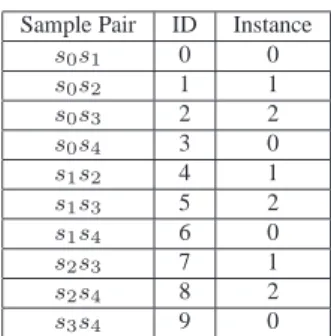
As mentioned before, each instance of the Edge filter may be responsible for one or more pairs of samples. Therefore, we had to establish some kind of strategy to distribute the pair of samples among them. To do that, we created a formula that was able to assign the pair of samples in a circular way, defining consecutive ids for the pair of samples. Then, to distribute them we just calculate the module in the number of instances. For example, let’s say we have 5 samples and 3 instances of the Edge filter. The corresponding id for each pair of samples, as well as the instance that is responsible for it, is shown in Figure 10.
Sample Pair ID Instance
s0s1 0 0 s0s2 1 1 s0s3 2 2 s0s4 3 0 s1s2 4 1 s1s3 5 2 s1s4 6 0 s2s3 7 1 s2s4 8 2 s3s4 9 0
Figure 10. Pair of samples and Instance mapping.
It’s important to point out that the same strategy is used in the Bicluster filter to distribute the pair of timestamps among the instances of this filter. Therefore, the formula used to generate these results in both cases are shown below: id= (Te∗ef)− (e f∗(ef + 3)) 2 +es−1, where:
• id is the identification number for that pair of elements (pair of samples in the Edge filter, and pair of timestamps in the Bicluster filter);
• Teis the total number of elements (total number of samples in the Edge filter, and total number of timestamps in the Bicluster filter);
• ef is the first element of the pair of elements;
• esis the second element of the pair of elements.
Based on this information, we created a function to map the data from the Ratio Filter to the Edge Filter (sending the ratio value of each gene for each pair of samples), and to map the data from the Edge Filter to the Bicluster Filter (sending its valid biclusters).
Besides, it also helped to create the functions for the labeled streams that are self-loops (among the Edge Filter instances and the Bicluster Filter instances themselves). In these cases, the strategy used is basically to follow the path in the depth first search, so that each instance with the pair of elements exey (where x < y), sends its information to the instances that have the pair of elementseyez(wherey < z). To do that, we just have to calculate the ids of all the pair of elements in which the first element begins withey and map the data to that instance.
4.3 Discussion
ParTriCluster is a good example of an efficient algorithm that exploits three parallelization strategies: data parallelism, task parallelism, and asynchrony.
The data parallelism happens by the instantiation of several copies of the same filter, each instance being re-sponsible for a data partition. As discussed, gene is the partitioning dimension for the first filter, sample is for the second filter, and time is for the third filter. Usually there is no partitioning for the fourth filter, which receives a small amount of data, and is responsible for generating the algorithm output.
Task parallelism is implemented through the filter pipeline, which is controled by the data dependencies. For ex-ample, an instance of the filter Bicluster does not need to wait for the determination of all biclusters to start sending tricluster candidates. As a consequence, it is possible that several tasks are being performed simultaneously.
Finally, ParTriCluster also exploits asynchrony, since the same task may be processed by several filter instances, such as searching the edges that determine a bicluster.
Again, one interesting observation is that ParTriCluster may be seem as two depth-first searches: the first deter-mines biclusters and the second deterdeter-mines triclusters. The strategy employed for both cases is very similar and is based on multiple simultaneous searches that traverse each search space. We believe that the approach proposed here is applicable to any depth-first search. Further, since we exploit three levels of parallelism, the implemen-tation is quite “elastic”, in the sense that it adapts automatically to a wide range of problem configurations with respect to the width and height of the searched problem space.
5 Experimental results
In this section we discuss experimental results of the execution of ParTriCluster on a PC-based cluster mining an actual dataset of gene expressions. We start by describing the dataset and experimental environment, and then discuss the results.
We employed a real dataset in order to evaluate our algorithm in an actual use scenario. Our dataset is from the yeast cell-cycle regulated genes project1. The goal of that project is to identify all genes whose mRNA levels are regulated by the cell cycle. We looked at the time slices for the Elutritration experiments. There are a total of 7679 genes whose expression value is measured from time 0 to 390 minutes at 30 minute intervals. Thus, there are 14 total time points. Finally, we use 13 of the attributes of the raw data as the samples, and we obtain a 3D expression matrix of size: T×S×G = 14×13×7679. We mined this data looking for triclusters with parameters mx = 50 (genes), my = 4 (samples), mz = 5 (time points), and we setǫ= 0.003.
Regarding the computational environment, all experiments were performed in a cluster of Athlon64 3200+ (2010 MHz) with 2Gb RAM, running Linux 2.6.8 and connected by a switched Gigabit Ethernet. We varied the number of instances of the filters reader, edge, and bicluster with the number of processors. Since the algorithm is divided into phases, we assigned one instance of each filter to each processor, so that we better exploit our computational resources. Our measurements indicate that they overlap in terms of simultaneous processing during a negligible amount of the execution time. Finally, since we have 14 samples in the dataset, our experimental configurations employ just the numbers of processors that are factors of 14, otherwise we would have static load imbalance.
1
0 1 2 3 4 5 6 7 8 9 10 0 2 4 6 8 10 12 14 Speedup Number of Processors Edge Bicluster
Figure 11. Speedup for Filters Edge and Bicluster
We start our analysis by looking at the speedups for the filters edge and bicluster. We focused our analysis on these two filters because they account for most of the processing costs. We analyze them in isolation because their execution is mutually exclusive from a temporal perspective, that is, the bicluster filter executes only after the edge filter resumes. The speedups for both filters are good, although we observe a trend towards reducing the efficiency of the parallelization as we increase the number of processors. We are going to understand better this trend in the remaining of this section.
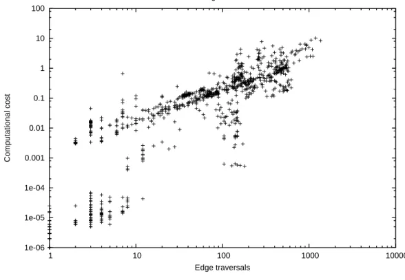
As mentioned before, the tricluster algorithm consists of two sets of depth-first searches, each set in a different range multigraph. Thus, it is important to first understand the nature of such searches and we are again going to evaluate the operations performed by the filters edge and bicluster separately. For sake of analysis, each search is a task, that is, a set of traversals towards defining a cluster. Our executions comprise 924 edge tasks and 1100 bicluster tasks. Each edge task traverses, on average, 149 multigraph edges, ranging from just 1 to 1360. Each bicluster task traverses, on average, 46 multigraph edges, ranging from 8 to 962. In both cases, the variability is quite high, presenting relative standard deviations of 130% and 290%, respectively. Further, when we analyze the computational costs associated with these tasks, the irregularity of the problem becomes more evident. The average processing time of an edge task is 0.44 seconds, while for a bicluster task is 0.30 seconds, but they vary significantly, since the most computationally expensive edge and bicluster tasks took 10 and 14 seconds, respectively. Figures 12 and 13 illustrate this variability. In each graph we plot, for a given task, its number of edge traversals and computational cost. We can clearly see a trend of increasing computational cost as we traverse more edges, but the variability is quite high. The explanation for such results is associated with the nature of the traversal-related operations. We perform a join of two lists for each traversal and the size of these lists vary significantly among searches and within a given search. The variation among searches is inherent to the problem, since clusters have variable frequency of occurrence, while the variation within a given search happens naturally
as we try to increase the cluster size and it becomes less frequent. Also, we do have a group of tasks, in both cases, that are characterized by few searches and very small computational costs. These are usually unsuccessfull searches in terms of not finding any clusters. All evidence presented so far makes clear that we are dealing with a hard problem in terms of parallelization, since its granularity varies significantly across datasets and even within a given execution. As we verify next, load imbalance is a major source of performance degradation, explaining the reduction in efficiency as we increase the number of processors.
1e-06 1e-05 1e-04 0.001 0.01 0.1 1 10 100 1 10 100 1000 10000 Computational cost Edge traversals Edge Tasks
Figure 12. Edge Tasks: Computational Cost×Edge Traversals
We now verify in detail the parallel execution results. We focus our analysis on the 14-processor execution. First, it is interesting to verify how many tasks each processor worked on and again we find that there is a high variability. Table I shows such number for both edge and bicluster tasks, where we can see its high variability. Similar information is given by analyzing the number of processors that participate in processing a given task (Figures 14 and 15), where we can see that tasks usually involve several processors, and this trend is stronger for the bicluster tasks.
As discussed, the Anthill environment allows the exploitation of three sources of parallelism. It is interesting to evaluate whether we are really exploiting these dimensions. Data and task parallelism are being exploited explicitly in the code, while asynchrony depends on the execution time conditions. In the case of ParTricluster, we may assess the amount of asynchrony by verifying the number of tasks that are being processed simultaneously. Figures 16 and 17 show the cumulative probability distribution of the number of tasks being processed simultaneously by 4 arbitrary instances of the edge and bicluster filters. From those graphs, We can see clearly that, regardless the instance, during half of the execution time we have 70 or more tasks being processed simultaneously for the edge filter. There is a similar situation for the bicluser filter, but the number is 30 in this case. Further, we should also note that the bicluster filters are inactive 30% of the execution time, as a consequence of a smaller computational demand. Again, this behavior is expected from the workload, since the edge filter joins lists of genes while the
1e-06 1e-05 1e-04 0.001 0.01 0.1 1 10 100 1 10 100 1000 Computational cost Edge traversals Bicluster Tasks
Figure 13. Bicluster Tasks: Computational Cost×Edge Traversals
tricluster filter joins lists of biclusters, which are usually smaller.
One last issue to evaluate is regarding the amount of load imbalance within a given task. We chose the most intensive task in terms of edge traversals (1360) from the filter edge for analysis. As expected, this task uses all processors, but it presents a significant amount of load imbalance. The task has a computational cost of 8.38 seconds. The number of edge traversals per processor range from 81 to 162, and the computational cost per processor from 0.003 to 3.258 seconds. Again, we could not establish a robust correlation among these two measures, although usually the greater the number of traversals, the larger is the computation time. It is also interesting to note that the life spam of task in a processor also varies significantly. For instance, in the processor that presented the largest computational cost, the task duration is smaller than in the processor with the smallest computational cost.
Thus, we may conclude that, given the irregularity of the problem, our Anthill-based implementation were very successfull, since we were able to achieve good speedups and use the processors quite efficiently. The load imbalance conditions in which the execution took place were severe, but our parallelization and Anthill were able to handle them well. The performance degradation we observed is due to not only this imbalance, but also the varying granularity of the tasks, which sometimes make the communication too expensive compared to the processing associated with it. One solution, being implemented, is to coalesce messages, so that we request more than one traversal per message. This solution will reduce our overhead while improving the efficiency of the solution, since we do have enough multiprogramming (that is, tasks being processed simultaneously) to hide the delays associated with the coalescing.
Proc. Edge Bic 0 355 864 1 420 865 2 385 787 3 385 943 4 385 710 5 381 866 6 381 785 7 505 707 8 318 629 9 342 785 10 342 707 11 342 786 12 354 786 13 354 630
Table I. Number of tasks per processor
6 Conclusions and future work
In this work we proposed and evaluated a parallel algorithm for clustering in three dimensions simultaneously, ParTriCluster. This algorithm is based on the filter-labeled-stream paradigm provided by Anthill. Experimental results demonstrated the algorithm scalability, with good speedups.
Our algorithm was able to achieve such scalability as a consequence of the simultaneous exploitation of several parallelism dimensions, namely data parallelism, task parallelism, and asynchrony. Further, the same strategy may be applied to any depth-first search, being a simple and efficient solution, also capable of adapting to a wide range of problem configurations.
We envise some future work directions. The first direction is towards devising new criteria for evaluating the quality of the triclusters generated and the relationship between tricluster quality and execution parameters. Although we achieved good results for the datasets tested, we still need to perform experiments in other datasets. In this case, some of the implementation decisions such as the labeling strategy for the streams may lead to load imbalance and consequently performance degradation, demanding novel labeling strategies that minimize such problems. Finally, this work motivated extensions to the Anthill environment, towards message coalescing, so that the asynchrony inherent to the applications may be exploited for reducing the communication overheads.
References
[1] Jacques Cohen. Bioinformatics - an introduction for computer scientists. ACM Comput. Surv., 36(2):122– 158, 2004.
[2] Lizhuang Zhao and Mohammed J. Zaki. Tricluster: An effective algorithm for mining coherent clusters in 3d microarray data. In SIGMOD Conference, pages 694–705, 2005.
[3] Amir Ben-Dor and Zohar Yakhini. Clustering gene expression patterns. Third annual international
0 20 40 60 80 100 120 140 160 180 2 4 6 8 10 12 14
Number of Edge Tasks
Processors
Number of Processors per Task
Figure 14. Edge Tasks: Number of Processors per Task
[4] Daxin Jiang, Jian Pei, and Aidong Zhang. Articles on microarray data mining: Towards interactive explo-ration of gene expression patterns. ACM SIGKDD Exploexplo-rations Newsletter, Volume 5 Issue 2, December 2003.
[5] Amos Tanay, Roded Sharan, and Ron Shamir. Discovering statistically significant biclusters in gene expres-sion data. Bioinformatics, pages S136–S144, 2002.
[6] Jinze Liu and Wei Wang. Op-cluster: Clustering by tendency in high dimensional space. 3rd IEEE
Interna-tional Conference on Data Mining, pages 187–194, 2003.
[7] T. M. Murali and Simon Kasif. Extracting conserved gene expression motifs from gene expression data.
Pacific Symposium on Biocomputing, pages 77–88, 2003.
[8] Sara C. Madeira and Arlindo L. Oliveira. Biclustering algorithms for biological data analysis: A survey.
IEEE/ACM Transactions on Computational Biology and Bioinformatics (TCBB), January 2004.
[9] A. Veloso, W. Meira Jr., R. Ferreira, and D. Guedes. Asynchronous and anticipatory filter-stream based parallel algorithm for frequent itemset mining. In ECML/PKDD 2004 Conference, pages 647–652. ACM Press, 2004.
[10] R. Ferreira, W. Meira Jr., D. Guedes, L. Drummond, B. Coutinho, G. Teodoro, T. Tavares, R. Araujo, and G. Ferreira. Anthill: A scalable run-time environment for data mining applications. In Proc. of the 17th
International Symposium on Computer Architecture and High Performance Computing, Rio de Janeiro, RJ,
0 50 100 150 200 250 300 350 2 4 6 8 10 12 14
Number of Bicluster Tasks
Processors
Number of Processors per Task
Figure 15. Bicluster Tasks: Number of Processors per Task
[11] Anurag Acharya, Mustafa Uysal, and Joel H. Saltz. Active disks: Programming model, algorithms and evaluation. In Architectural Support for Programming Languages and Operating Systems, pages 81–91, 1998.
[12] Michael Beynon, Renato Ferreira, Tahsin M. Kurc, Alan Sussman, and Joel H. Saltz. Datacutter: Middleware for filtering very large scientific datasets on archival storage systems. In IEEE Symposium on Mass Storage
0 0.1 0.2 0.3 0.4 0.5 0.6 0.7 0.8 0.9 1 0 20 40 60 80 100 120 140 160 180
Cumulative distribution of execution time
Tasks being processed Edge Tasks
Figure 16. Edge Simultaneous Tasks
0.3 0.4 0.5 0.6 0.7 0.8 0.9 1 0 10 20 30 40 50 60 70
Cumulative distribution of execution time
Tasks being processed Bicluster Tasks