Procedia Computer Science 36 ( 2014 ) 246 – 253
1877-0509 © 2014 Published by Elsevier B.V. This is an open access article under the CC BY-NC-ND license (http://creativecommons.org/licenses/by-nc-nd/3.0/).
Peer-review under responsibility of scientific committee of Missouri University of Science and Technology doi: 10.1016/j.procs.2014.09.087
ScienceDirect
Available online at www.sciencedirect.com
Complex Adaptive Systems, Publication 4 Cihan H. Dagli, Editor in Chief
Conference Organized by Missouri University of Science and Technology 2014 - Philadelphia, PA
Volatility Forecasting using a
Hybrid GJR-GARCH Neural Network Model
Soheil Almasi Monfared
a, David Enke
b,*aMissouri University of Science and Technology, 223 Engineering Management Rolla, MO 65409-0370, USA bMissouri University of Science and Technology, 227 Engineering Management, Rolla, MO 65409-0370, USA
1. Introduction
Volatility modeling and forecasting is an important step when studying financial time series. It is also critical in hedging and pricing financial instruments. Some econometric models attempt to model the volatility of financial returns. One of the pioneering works was the Generalized Auto Regressive Conditional Heteroskedasticity (GARCH) model, which was introduced by Bollerslev in 1986 [1]. Some studies indicated that negative returns or bad news has a bigger impact on volatility than positive returns or good news [2,3,4]. Some asymmetric versions of the GARCH model have been developed to address this observation [5,6,7]. There are a number of studies that try to compare the GARCH model versus its asymmetric versions. Many of these studies found that asymmetric GARCH models outperform classic GARCH [9, 10, 11]. Awartani and Corradi found that asymmetric models outperform the GARCH in forecasting one step ahead and multi-step ahead, such that the forecasting advantage ofasymmetric models versus the GARCH in multi-step ahead is not as significant as one step ahead [9]. Brownlees et al. introduces the Glosten Jagannathan and Runkle (GJR) model as a threshold autoregressive conditional
Corresponding author. Tel: +1-573-341-4749 E-mail address: [email protected]
Abstract
Volatility forecasting in the financial markets, along with the development of financial models, is important in the areas of risk management and asset pricing, among others. Previous testing has shown that asymmetric GARCH models outperform other GARCH family models with regard to volatility prediction. Utilizing this information, three popular Neural Network models (Feed-Forward with Back Propagation, Generalized Regression, and Radial Basis Function) are implemented to help improve the performance of the GJR(1,1) method for estimating volatility over the next forty-four trading days. During training and testing, four different economic cycles have been considered between 1997-2011 to represent real and contemporary periods of market calm and crisis. In addition to stress testing for different neural network architectures to assess their performance under various turmoil and normal situations in the U.S. market, their synergy along with another econometric model is also accessed.
© 2014 The Authors. Published by Elsevier B.V.
Selection and peer-review under responsibility of scientific committee of Missouri University of Science and Technology. Keywords: Volatility Forecasting, Asymmetric GARCH, Radial Basis Functions, Stress Testing
© 2014 Published by Elsevier B.V. This is an open access article under the CC BY-NC-ND license (http://creativecommons.org/licenses/by-nc-nd/3.0/).
heteroskedasticity (TARCH) model and found it to be the best forecaster among asymmetric models and GARCH for one step or multi-step ahead forecasting [6]. Their study also suggests that updating parameters weekly and considering as many observations as possible provides benefits. Unfortunately, this is often impractical for risk management purposes since projected volatility is usually considered for longer periods, with one or two months being more adequate. The combination of econometric methods with other methods to improve forecasting performance is considered in [12, 13, 14, 15, 18], with each finding that the hybrid model is more efficient than the classic econometric model. In particular, a GARCH model combined with neural networks outperforms GJR-GARCH and GJR-GARCH [16]. In [17], a simple two neuron hidden layer perceptron was tested in combination with GARCH, illustrating the benefits of a simple neural network. Finally, [19] found that GJR outperforms other GARCH family models, while the radial basis function (RBF) networks outperform multi-layer perceptron in volatility forecasting. What makes our study different from [16,17,19] is the longer forecasting period without updating the trained model. The other differentiating feature is the testing of three different architectures in a hybrid model, in four different economic cycles. This study aims to assess the performance of three different architectures when they are utilized to improve a GJR-GARCH volatility-forecasting model. This is in a line with what has found - that an artificial neural network with a dynamic architecture outperforms the ARCH and a multilayer perceptron neural network [21].
2. Methodology
2.1 Data
The dataset used for modeling includes the daily return and variance of ten NASDAQ indices, namely, Bank, Biotechnology, Composite, Computer, Industrial, Insurance, Other Finance (non-Bank), Telecommunication, Transportation, and the NASDAQ 100 from 1/8/1997 to 9/1/2011. The ten indices were chosen to cover almost the entire economy and import as much information as possible to the hybrid model. The entire study time period was split into four sub-periods to test the hybrid model’s performance under various economic situations. This allows observation of how different neural network architectures work in various financial environments, including crisis. This is similar to scenario analysis for stress testing during financial risk management, allowing for the assessment of the forecasting ability of three popular neural networks architectures in financial forecasting in combination with an econometric method. The econometric model utilized is an asymmetric GARCH model, GJR, which has been widely used in volatility forecasting either alone or within hybrid models [9,13,16]. Finally, the squared return is used as a proxy for volatility (variance) [20].
The first period tested extended from 1/8/1997 to 3/10/2000, starting with the dot-com boom. The Russian financial crisis happened near the middle of this period in 1998. The period includes 800 observations, allowing the hybrid model to learn from the economic environment. The ten NASDAQ index variances in this time interval form the first training dataset. The model is tested by forecasting the variance of the NASDAQ Composite index over the next 44 trading days from 3/13/2000 to 5/12/2000. This is the first dataset tested that includes the dot-com bust in 2000. The 44 trading days represent approximately two calendar months. While this is a long period of forecasting for a model without updating, it is common in the options market to have a volatility prediction for the next two months. While ten indices are under consideration, it is impossible to show each volatility profile in this paper. Thus, the NASDAQ Composite index volatility is shown in Figures 1 and 2 as an example. Another reason for focusing on this index is that its index variance is also going to be forecasted. The second period tested is from 1/3/2002 to 11/3/2003 and begins after the dot-com crash. This period includes 460 observations, allowing the hybrid model to learn from the economic environment. The ten aforementioned NASDAQ index variances in this time interval form the second training dataset. Once again, the model is tested by forecasting the next 44 trading days’ variance in the NASDAQ Composite index from 11/4/2003 to 1/7/2004. This is the second testing dataset which includes data after the market crash, and could be considered a period of calm and recovery after the tech-included market correction. The NASDAQ Composite index volatility is shown in Figure 3.
Fig.1. NASDAQ Composite Index Volatility from 1997 to 2000 (one part of the training dataset)
Fig.2. NASDAQ Composite Index Volatility from 3/2000 to 5/2000 (out-of-sample testing dataset)
Fig.3. NASDAQ Composite Index Volatility from 11/2003 to 1/2004 (out-of-sample testing dataset)
The third period tested is from 1/4/2005 to 5/27/2008 and starts with the U.S. real estate market rally, driven in part by subprime mortgages lending and the expansion of asset back securities popularity in the fixed income market. This period includes 854 observations and again allows the hybrid model to learn from the economic environment. As before, the ten NASDAQ index variance levels in this time interval form the third training dataset. The model is then tested by forecasting the next 44 trading days’ variance in the NASDAQ Composite index from 5/28/2008 to 7/29/2008. This is the third testing dataset that includes part of the credit crisis crash period and could be considered a turbulent period after a recovery and subsequent bull market. The NASDAQ Composite index volatility is shown in Figure 4.
Fig.4. NASDAQ Composite Index Volatility from 5/2008 to 7/2008 (out-of-sample testing dataset)
The fourth period tested is from 1/5/2010 to 6/30/2011 and starts two-years after credit crisis introduced recession. This period includes 376 observations, enough to allow the hybrid model to learn from the economic environment. The ten NASDAQ index variances in this time interval form the last training dataset. As before, the model is tested by forecasting the next 44 trading days’ variance in the NASDAQ Composite index from 7/1/2011 to 9/1/2011. This last testing dataset includes part of the sovereign debt crisis in Europe after the financial crisis. The NASDAQ Composite index volatility is shown in Figure 5.
Fig.5. NASDAQ Composite Index Volatility from 7/2011 to 9/2011 (out-of-sample testing dataset) 2.2 GJR
Glosten et al. introduced the GJR model in 1993 [6]. It is classified as an asymmetric version of GARCH that takes into account the asymmetric nature of investor response to stock or index returns (percentage change). For this study, there is one lag in return and one lag in variance, thus a GJR(1,1) model was utilized.
(1) 1 1 − −
−
=
t t t tp
p
p
r
is the percentage change in the index level at time t in comparison with time t-1, or return at time t. The “I” is an indicator function that is equal to 1 ifr
t<
0
and 0 otherwise. 21 2&
+ t
t
σ
σ
are variances at time t and forecasted variance for time t+1, respectively. Using this model requires solving the following optimization as a maximum likelihood estimator in order to find four parameters.2 2 2 1 ( (t 0))t t t
ω
α
γ
I r rβσ
σ
+ = + + < +Max ω,α,γ,β −ln(σi 2)−(ri 2 σi 2) i
∑
⎡ ⎣ ⎢ ⎢ ⎤ ⎦ ⎥ ⎥ s.t. ω>0, α ≥0, α+γ ≥0, β ≥0, α+ 1 2γ+β<1 (2)The last constraint is added according to [8] to be covariance stationary. The MATLAB optimization toolbox was used for solving the above optimization. A total of 10 optimizations were solved for each period, totaling 40 optimizations being run to find the optimum parameter set (
ω
*,
α
*,
γ
*,
β
*) for each of the ten NASDAQ indexes during each of the four defined periods. Using machine learning terminology, this is equivalent to training the GJR-GARCH model for each index during each period.2.3 Hybrid Model
Improving the GJR-GARCH performance for volatility forecasting is the main goal of this research. Nonetheless, the distinguishing feature of this research is testing different architectures in different economic situations (mostly crisis) by building a hybrid model for a 44 step ahead forecast. The long forecasting period was considered without updating the model (two calendar months, or 44 trading days). The neural network model building approach is in line with the GJR-GARCH econometric model, which means the neural network is trained and tested based on the outputs (forecasts) of GJR-GARCH model. In total, testing includes 12 neural networks (hybrid models), consisting of three neural networks for each of the four defined time periods. Specifically, Feed-Forward with Back Propagation (FFBP), Generalized Regression (GR), and the Radial Basis Function (RBF) neural networks were tested to find the most efficient hybrid model combination of GJR-GARCH and Neural Network for each time period. These networks were considered because of their extensive application in financial forecasting. The combination process is depicted in Figure 6.
A total of 20 neurons in one hidden layer and one output neuron are considered for the Feed-Forward with Back Propagation (FFBP) network. Testing included 10, 15, and 25 neurons in hidden layer, but 20 neurons made the network performance higher (smaller MSE). Because of the positive nature of volatility, the LogSig function was chosen for hidden and output neurons. Generalized Regression (GR) and Radial Basis Function (RBF) networks were trained by MATLAB as well, using Gaussian activation functions that are consistent with GJR-GARCH assumptions. The spread constant was set equal to 1 and the performance goal was set to 3*10-6, similar to what is used in MLE optimization of GJR-GARCH as an initial value for omega.
Fig.6. Hybrid Model
3. Results
The optimum parameters for GJR-GARCH have been computed for each index in each period (a total of 40 optimum parameter sets). Considering the third period, index volatilities were more sensitive to previous negative returns, rather than previous returns. For 6 indices out of 10, alpha is equal to zero. This is also seen for 2 out of 10 indices for the first period, 5 out of 10 indices for the second period, and 4 out of 10 indices in the fourth period. The
10 dimentional input vector of GJR-GARCH volatility forecasts for 10 indices
FFBP/GR/RBF NASDAQ Composite Index Volatility forecast
different tested architectures with modeling details are reported in Table 1. As mentioned earlier, 12 different architectures have been tested. Tables 2-5 show the performance of the hybrid models for the four previously defined time periods. Percentage change in MSE represents the improvement that the hybrid model attained in decreasing the GJR-GARCH forecasting MSE for the out-of-sample dataset (larger negative percentage is desired). Table 1. Three Different Architectures in Four Different Time Periods
Time Period 1997-2000 2002-2003 2005-2008 2010-2011
FFBP 20 Log-Sig hidden neurons
1 Log-Sig output neuron Trainlm method
20 Log-Sig hidden neurons
1 Log-Sig output neuron Trainlm method
20 Log-Sig Hidden neurons
1 Log-Sig output neuron Trainlm method
20 Log-Sig hidden neurons
1 Log-Sig output neuron Trainlm method GR 800 Gaussian neurons
1 Purelin output neuron
460 Gaussian neurons 1 Purelin output neuron
854 Gaussian neurons 1 Purelin output neuron
376 Gaussian neurons 1 Purelin output neuron RBF 2 Gaussian neurons 2 Gaussian neurons 2 Gaussian neurons 2 Gaussian neurons Table 2. Hybrid Model Performance in the First Time Period using Different Architectures
1997-2000 MSE for GJR(1,1) Forecasting MSE for Hybrid Model Percentage Change in MSE
FFBP 5.41623E-06 8.23979E-06 52.13%
GR 5.41623E-06 5.30669E-06 -2.02%
RBF 5.41623E-06 5.04768E-06 -6.80%
The RBF is the most efficient architecture for the period from 1997-2000 by reducing the MSE by almost 7%. Table 3. Hybrid Model Performance in the Second Time Period using Different Architectures
2002-2003 MSE for GJR(1,1) Forecasting MSE for Hybrid Model Percentage Change in MSE
FFBP 4.10804E-08 8.67522E-06 21017.63%
GR 4.10804E-08 8.05717E-08 96.13%
RBF 4.10804E-08 4.48362E-08 9.14%
For the 2002-2003 period, the RBF architecture is the best of the group, but none of the neural networks could decrease the mean squared error. All of the networks made the accuracy worse.
Table 4. Hybrid Model Performance in the Third Time Period using Different Architectures
2005-2008 MSE for GJR(1,1) Forecasting MSE for Hybrid Model Percentage Change in MSE
FFBP 1.14901E-07 1.91136E-06 1563.48%
GR 1.14901E-07 9.27189E-08 -19.31%
RBF 1.14901E-07 8.81455E-08 -23.29%
The RBF is the most efficient architecture for the period from 2005-2008. It reduced the MSE by about 24%. Table 5. Hybrid Model Performance in the Fourth Time Period using Different Architectures
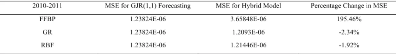
2010-2011 MSE for GJR(1,1) Forecasting MSE for Hybrid Model Percentage Change in MSE
FFBP 1.23824E-06 3.65848E-06 195.46%
GR 1.23824E-06 1.2093E-06 -2.34%
The GR is the most efficient architecture for the period from 2010-2011. The improvement is not as good as the other periods, but the hybrid model still outperforms the GJR-GARCH model.
4. Conclusions
Based on the testing results of the various models over the four defined time periods, it is possible to draw some conclusions:
1) In extreme turmoil conditions, such as the 2008 financial crisis, two neural networks architectures improved the forecasting ability of the GJR-GARCH more than they did in the 2000 crash. It seems that the hybrid models are more useful in extreme event forecasting because as the structure of volatility process becomes more complex. This could not be explained simply by using an econometric model, but instead needed a more complex model (such as the hybrid model) to better explain the volatility. Considering frequency and timing of the volatility process is recommended to realize its structure.
2) The hybrid model is a good candidate for use along with the CVaR measure in portfolio risk management. CVaR tries to model the expected loss under the worst-case scenario. The hybrid model has shown the ability to predict the volatility in such cases.
3) In low volatility periods, it is recommended that neural networks architectures, as well as the GJR, not be used for forecasting purposes. The hybrid model is not beneficial due to the unnecessary complexity of the model. An explanation could be in the training period when the hybrid model learns from the after crisis conditions so high volatility is memorized and is projected for the forecasting period. This causes an overestimation of volatility.
4) Using a feed-forward neural network with back propagation learning is not recommended in combination with the GJR-GARCH for volatility forecasting under any circumstances (economic conditions). This is a direct outcome of the hybrid model performance, as tested in Tables 2, 3, 4 and 5 (line 1).
5) Each crisis has its own characteristics, so there is no best architecture for forecasting volatility better than the other when in combination with the GJR-GARCH. Comparing results in Tables 2, 4 and 5 indicate that the Generalized Regression and Radial Basis Function networks have advantages in some time periods (such as crisis), but neither is absolutely more accurate. On the other hand, some studies have found that the return distribution in financial time series tend to be fat tail instead of a normal distribution. This can be translated into the context of neural networks that possibly another activation functions instead of a Gaussian activation function should be used. It is consistent with [21] that distinguish a dynamic architecture.
6) All data mining methods have limitations. Figure 7 shows this very well. The following graph shows the hybrid model MSE (using the RBF network) compared to the GJR-GARCH MSE. The difference is not great, but the improvement is obvious. It was not possible to model and explain all the index volatility. Nonetheless, increasing the accuracy by 1% is a competitive advantage in financial markets when the scale of investments is in millions or billions of dollars.
7) Multi-variable performance measures (such as AIC) can assess the efficiency of having 9 more input variables in volatility forecasting in order to compare different architectures. Using these measures is recommended for future research.
Fig.7. Hybrid Model Squared Errors in Forecasting versus GJR Squared Errors
References
1. T. Bollerslev, “Generalized Auto Regressive Conditional Heteroskedasticity”, Journal of Econometrics, vol. 31, no. 3, pp. 307- 327, (1986).
2. K. R. French, G.W. Schwert, R.F. Stambaugh, “Expected stock returns and volatility”, Journal of Financial Economics, vol. 19, pp. 3-29, (1987).
3. A. A. Christie, “The stochastic behavior of common stock variances: Value, leverage, and interest rate effects”, Journal of Financial Economics, vol. 10, pp. 407-432, (1982).
4. F. Black, “Studies in stock price volatility changes”, Proceedings of the 1976 meeting of the business and economic statistics section, pp. 177-181, (1976).
5. D. B. Nelson, “Conditional Heteroskedasticity in Asset Returns: A New Approach”, Econometrica, vol. 59, no. 2, pp. 347-370, (1991). 6. L. Glosten, R. Jagannathan, and D. Runkle, “On the relationship between the expected value and the volatility of the nominal excess
return on stocks”, Journal of Finance, vol. 48, no. 5, pp. 1779-1801, (1993).
7. J. M. Zakoian, “Threshold heteroskedasticity models”, Journal of Economic Dynamics and Control, vol. 18, pp. 931-955, (1994). 8. L. Hentschel, “All in the family: nesting symmetric and asymmetric GARCH models”, Journal of Financial Economics, vol. 39, pp.
71-104, (1995).
9. B. M. A. Awartani, V. Corradi, “Predicting the volatility of the S&P-500 stock index via GARCH models: the role of asymmetries”,
International Journal of Forecasting, vol. 21, pp. 167-183, (2005).
10. C. Brownlees, R. Engle, B. Kelly, “A practical guide to volatility forecasting through calm and storm”, The Journal of Risk , vol. 14, no. 2, pp. 3-22, (2011/12).
11. D. Alberga, H. Shalita, R. Yosef, “Estimating stock market volatility using asymmetric GARCH models”, Applied Financial Economics, vol. 18, pp. 1201-1208, (2008).
12. R. G. Donaldson, and M. Kamstra, “An artificial neural network-GARCH model for international stock return volatility”, Journal of Empirical Finance, vol. 4, no. 1, pp. 17-46, (1997).
13. P. Ou, H. Wang, “Modeling and Forecasting Stock Market Volatility by Gaussian Processes based on GARCH, EGARCH and GJR Models”, Proceedings of the World Congress on Engineering, vol. 1, (2011).
14. J. K. Mantri, P. Gahan, B. B. Nayak, “Artificial Neural Networks - An Application to Stock Market Volatility”, International Journal of Engineering Science and Technology, vol. 2, no. 5, pp. 1451-1460, (2010).
15. A. Tarsauliya, R. Kala, R. Tiwari, A. Shukla, “Financial Time Series Volatility Forecast Using Evolutionary Hybrid Artificial Neural Network”, Advances in Network Security and Applications, Springer, pp. 463-471, (2011).
16. Y. H. Wang, “Nonlinear neural network forecasting model for stock index option price: Hybrid GJR–GARCH approach”, Expert Systems with Applications, vol. 36, pp. 564-570, (2009).
17. W. Kristjanpoller, A. Fadic, M.C. Minutolo, “Volatility forecast using hybrid Neural Network models”, Expert Systems with Applications, vol. 41, pp. 2437-2442, (2014).
18. M. Bildirici, Ö. Ö. Ersin, “Improving forecasts of GARCH family models with the artificial neural networks: An application to the daily returns in Istanbul Stock Exchange”, Expert Systems with Applications, vol. 36, pp. 7355-7362, (2009).
19. A. K. Dhamija, V. K. Bhalla, “Financial Time Series Forecasting: Comparison of Neural Networks and ARCH Models”, International Research Journal of Finance and Economics, vol. 49, pp. 194-212, (2010).
20. T. G. Andersen, T. Bollerslev, “Answering the skeptics: Yes, standard volatility models do provide accurate forecasts”, International Economic Review, vol. 39, pp. 885-905, (1998).
21.J D. Velasquez, S. Gutierrez, C. J. Franco, “Using A Dynamic Artificial Neural Network For Forecasting The Volatility Of A Financial Time Series”, Revista Ingenierias Universidad de Medellin, vol. 12, no. 22, pp. 125-132, (2013).