Support Vector Machines and Artificial Neural Networks: Assessing the Validity of Using Technical Features for Security Forecasting

(1)

Technological University Dublin Technological University Dublin

ARROW@TU Dublin

Dissertations School of Computing

2016-10-01

Support Vector Machines and Artificial Neural Networks:

Assessing the Validity of Using Technical Features for Security

Forecasting

James DiPadua

Technological University Dublin

Follow this and additional works at: https://arrow.tudublin.ie/scschcomdis

Part of the Computer Engineering Commons

Recommended Citation Recommended Citation

Di Padua, J.(2016) Support Vector Machines and Artificial Neural Networks: Assessing the Validity of Using Technical Features for Security Forecasting, Dissertation submitted in partial fulfilment of the requirements of Technological University Dublin for the degree of M.Sc. in Computing (Data Analytics), August 2016.

This Dissertation is brought to you for free and open access by the School of Computing at ARROW@TU Dublin. It has been accepted for inclusion in Dissertations by an authorized administrator of ARROW@TU Dublin. For more information, please contact

[email protected], [email protected], [email protected].

(2)

Support Vector Machines and Artificial

Neural Networks: Assessing the Validity of

Using Technical Features for Security

Forecasting

James DiPadua

A dissertation submitted in partial fulfilment of the requirements of Dublin Institute of Technology for the degree of

M.Sc. in Computing (Data Analytics)

(3)

DECLARATION

I certify that this dissertation which I now submit for examination for the award of MSc in Computing (Data Analytics), is entirely my own work and has not been taken from the work of others save and to the extent that such work has been cited and acknowledged within the test of my work.

This dissertation was prepared according to the regulations for postgraduate study of the Dublin Institute of Technology and has not been submitted in whole or part for an award in any other Institute or University. The work reported on in this dissertation conforms to the principles and requirements of the Institute’s guidelines for ethics in research.

I hold no positions, short or long, in any of the firms included in this study, nor was the work sponsored by any third-party entity. Further, this research is not intended to be construed as providing or implying investment advice.

Signed: _____________________________________ James DiPadua

(4)

Abstract

Stock forecasting is an enticing and well-studied problem in both finance and machine learning literature with linear-based models such as ARIMA and ARCH to non-linear Artificial Neural Networks (ANN) and Support Vector Machines (SVM). However, these forecasting techniques also use very different input features, some of which are seen by economists as irrational and theoretically unjustified. In this comparative study using ANNs and SVMs for 12 publicly traded companies, derivative price “technicals” are evaluated against macro- and microeconomic fundamentals to evaluate the efficacy of model performance. Despite the efficient market hypothesis positing the ill-suitability of technicals as model inputs, this study finds technical indicators to be nearly as performant as fundamentals at forecasting the future prices of a security. Additionally, all model predictions were fed into an automated trading machine and evaluated against a simple Buy-and-Hold, finding model performance at par with the passive Buy-and-Hold investment strategy.

Key Words: Stock Forecasting, Feature Selection, Support Vector Machine, Artificial Neural Networks

(5)

Acknowledgments

First, a big thank you to each of my professors for positioning me to complete this work. I'd like to thank Dr. Luca Longo for his steadfast insistence on a process for successfully completing this research and thesis. His insight and experience were exceptionally helpful. I am also appreciative of Dr. John McAuley's early support in encouraging me to pursue this topic in financial forecasting. His patience, counsel and affable pragmatism were instrumental for this project.

Last, and most importantly, I am eternally thankful to my wife Adria Mooney for encouraging me to pursue this course of study. She helped me see that the project could be completed without interfering with my ability to be a husband and father--and made sure that happened!

(6)

3.6.1. Strengths………...52 3.6.2. Weaknesses...…...…...…...…...…...…...…...…...…...…...………53 4. Implementation / Results...…...…...…...…...…...…...…...…..…...…...……….55 4.1. Software...…...…...…...…...…...…...…...…...…...…...….………..55 4.2. Data Exploration...…...…...…...…...…...…...…...…...…....…...……….55 4.2.1. Technical Indicators……….56 4.2.2. MicroEconomic Indicators………...58 4.2.3. MacroEconomic Indicators………..59 4.3. Data Preparation...…...…...…...…...…...…...…...…...…...…...………..61 4.4. Data Modeling...…...…...…...…...…...…...…...…...…...…...……….62 4.5. Model Validation...…...…...…...…...…...…...…...…...…...…...……….65 4.5.1. SVR Model...…...…...…...…...…...…...…...…...…...…...……….65 4.5.2. ANN Model...…...…...…...…...…...…...…...…...…...…...………69

4.6. Model Prediction & Visualization...…...…...…...…...…...…...…...…...…...…..73

5. Evaluation / Analysis...…...…...…...…..…...…...…...…...…...…...………...85

5.1. Evaluation of Results...…...…...…...…...…...…...…...…...…...…...…………...85

5.2. Observations from the Results...…...…...…...…...…...…...…...…...…...………86

5.3. Strengths of the Results...…...…...…...…...…...…...…...…...…...…...………...87

5.4. Limitations of the Results...…...…...…...…...…...…...…...…...…...…...………87

6. Conclusions and Future Work…...…...…...…...…...…...…...…...…...…...……….89

6.1. Summary...…...…...…...…...…...…...…...…...…...…...……….89

6.2. Contribution and Impact...…...…...…...…...…...…...…...…...…...…...……….90

6.3. Future Work...…...…...…...…...…...…...…...…...…...…...………90

7. Bibliography...…...…...…...…...…...…...…...…...…...…...………...93

8. Appendix A: Feature Correlation Heatmaps...…...…...…...………..105

9. Appendix B: Visualizing Price and Economic Indicators...…...…...…...…………..109

(8)

Table of Figures

Figure 2.1 Security Price Forecasting Landscape…...…...……….……… 14

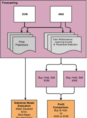
Figure 3.1 Study Design and Methodology…...…...…...…...………... 35

Figure 3.2 S&P500, 2006 through 2015 ...…...…...…...…...……… 40

Figure 3.3 Security Forecasting Workflow……...…...…...……… 50

Figures 4.1 AT&T and Microsoft, Closing Price and Moving Averages, 2015………...56

Figure 4.2 AT&T, Feature Correlation Heatmap………57

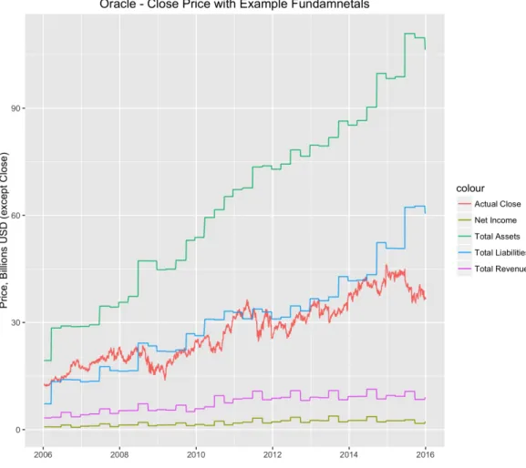
Figure 4.3 Oracle, Closing Price and Changes in Fundamentals, 2006 - 2015………...58

Figure 4.4 S&P500, 2006 through 2015...…...…...…...…...………60

Figure 4.5 LIBOR, 2006 - 2015.…………...…...…...…...………60

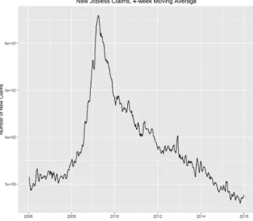
Figure 4.6 New Jobless Claims, 4-week Moving Average, 2006 - 2015..……….61

Figure 4.7 Civilian Labor Participation, 2006 - 2015………...61

Figure 4.8 Three SVR Models Performances by RMSE………...68

Figure 4.9 Three ANN Models Performances by RMSE………..72

Figure 4.10.a, b Microsoft, Forecasts vs Actual, Technicals Only……….... 74

Figure 4.11.a, b Exxon, Forecasts vs Actual, Technicals Only………...75

Figure 4.12.a, b Ford, Forecasts vs Actual, Technicals Only.………...76

Figure 4.13.a, b McDonald's, Forecasts vs Actual, Fundamentals Only………...77

Figure 4.14.a, b AT&T, Forecasts vs Actual, Technicals…. Only………...……...78

Figure 4.15.a, b Chevron, Forecasts vs Actual, Fundamentals Only………...…...79

Figure 4.16.a, b AT&T, Forecasts vs Actual, Fundamentals Only…….………...…..80

Figure 4.17.a, b Ford, Forecasts vs Actual, Fundamentals Only……..………...…... 81

Figure 4.18.a, b McDonald's, Forecasts vs Actual, Blended Model....………... 82

Figure 4.19.a, b Exxon and Chevron, Forecasts vs Actual, Blended Model……….……..83

Figure 4.20.a, b AT&T, Forecasts vs Actual, Blended Model…...…….………...…..84

Figure 4.21.a, b Ford, Forecasts vs Actual, Blended Model…...……..………...…...85

Table of Tables

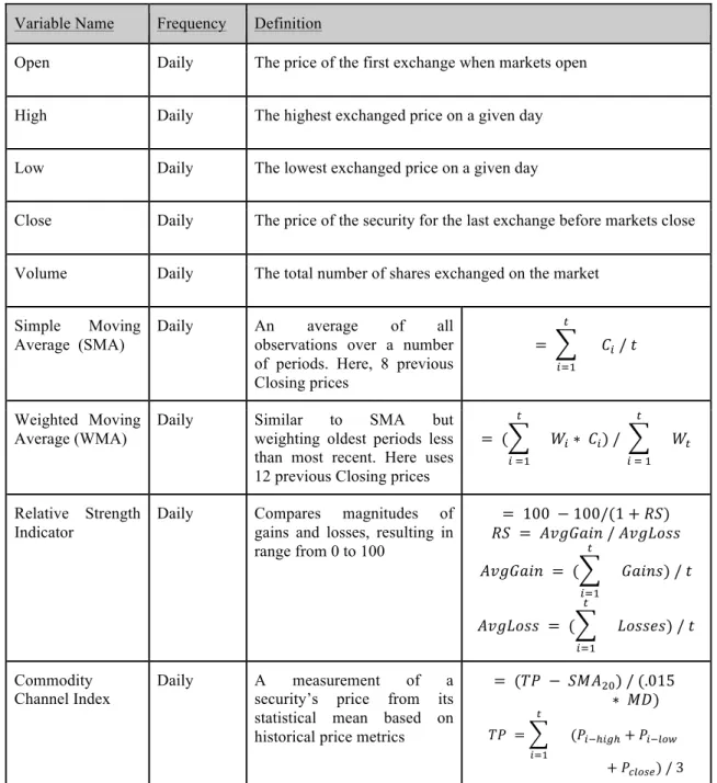
Table 3.1: Example Technical Indicators……...…...…...…...…...…...…...…...… …...27

Table 3.1: Studied Companies…...…...…...…...…...…...…...…...…...…...…...… …...37

(9)

Table 3.3: Microeconomic Indicators…...…...…...…...…...…...…...…...…...…...……. 45 Table 3.4 : Technical Features…...…...…...…...…...…...…...…...…...…...………….... 48 Table 4.1 : SVR Experiment 1 -- Technical Features Only…...…...…...…...…...…...… 66 Table 4.2: SVR Experiment 2 -- Fundamental Features Only…...…...…...…...…...…....67 Table 4.3 : SVR Experiment 3 -- Blended, Technical and Fundamental …...…...…...… 68 Table 4.4 : ANN Experiment 1 -- Technical Features Only…...…...…...…...…...…...… 70 Table 4.5 : ANN Experiment 2 -- Fundamental Features Only…...…...…...…...…...….. 71 Table 4.6 : ANN Experiment 3 -- Blended, Technical and Fundamental………...72

List of Acronyms

ANN - Artificial Neural Networks

ARMA / ARIMA - Autoregressive Moving Average, Autoregressive Interval- ARCH / GARCH - Autoregressive

BAH - Buy-and-Hold

CCI - Commodity Channel Index DJIA - Dow Jones Industrial Average EMH - Efficient Market Hypothesis

FF-NN / BP-NN - Forward Feed Neural Network, Backpropagation- MA / SMA/ WMA - Moving Average, Simple-, Weighted-

MACD - Moving Average Convergence/Divergence MSE / RMSE - Mean Squared Error, Root-

MAE - Mean Absolute Error NYSE - New York Stock Exchange RSI - Relative Strength Indicator S&P500 - Standard & Poor's 500

(10)

1. Introduction

Financial security exchange markets, “stock markets,” are large, volatile and seemingly chaotic (Huang, Nakamori and Wang, 2005; Wang, Wang, Zhang and Guo, 2011; Vui, Soon, On, and Alfred, 2013). The allure of identifying inflection points, being able to time the market, and to reduce risk yet maintain or increase profitability through participation in stock markets has generated immense interest among investors and researchers alike. The presence of the financial markets can be felt in nearly every sector of the economy, in nearly every corner of the world, attracting researchers from finance and economic interests and also from statistics and machine learning practitioners. The event-horizon-like nature of the financial markets, pulling all economic and social actors into its gravitational force is even examined in social justice and ecology research (Galaz, Gars, Moberg, Nykvist and Repinski, 2015). In 2013, according to Galaz, Gars, Moberg, Nykvist and Repinski (2015), the total wealth under professional management (investment firms, sovereign wealth funds, hedge funds, mutual funds, etc) reached 68.7 trillion USD, or approximately 18 times the national GDP of Germany for 2015 and approximately three times the total 2014 GDP for the entire EuroZone (CIA; TradingEconomics).

Indeed, the financial markets permeate every facet of contemporary life, and as a consequence of this pervasiveness, locating the opportunities for entering and exiting a position using advanced statistical and machine learning techniques has garnered much research and investment attention. While this paper does not seek to provide a specific answer to whether stock markets might be predicted or to evaluate every facet through which a security might be valued, the research intent is to provide a single answer to a simple question: do historical prices conveyed through technical factors such as moving averages allow a machine-based algorithm to accurately forecast stock prices?

1.1. Project Background

There are markets around the world where securities are exchanged daily between investors. The primary goal with these exchanges is to extract a profit, often through price arbitrage, a process of seeking a price differential between what one investor is willing to

(11)

pay and what another perceives as the intrinsic value of the security (Refenes, Zapranis and Francis, 1994). However, determining the intrinsic value of a security is non-trivial, subject to extensive research and heated debate (Fama, 1965; Fama and French, 1988; Shleifer and Summers, 1990; Mankiw, Romer and Shapiro, 1991). Because of the complex, time-variant, non-trivial nature of security price forecasting, as well as the profit motive, security price forecasting is extensively present in machine learning literature (Atsalakis and Valavanis, 2009). Security forecasting is an alluring problem space for multiple reasons, mostly notably the promise for investment profit with reduced risk exposure. From a research perspective, security price forecasting is also an exciting area due to its inherent complexity--to accurately predict the movement of a stock or commodity is to not just “see the future” but to instill a structure to what frequently manifests itself as an erratic maelstrom of randomness.

As explored in more detail in the Literature Review many models rely extensively upon the use of historically derivative technical features--that is, model input features extrapolated from past security closing prices. Examples of these derivative features are frequently classified as Moving Averages. These, among other derivative technical features, are explained in more detail in chapter three, 'Design/Methodology.' In brief, however, it is worth noting that this class of features, from the perspective of economic theory, is “non-rational” because stock prices show a non-time dependency, or a "Random Walk" (Fama, 1965; Fama and French, 1988). It is from this perspective that the research question is posed.

The following research will seek to forecast the closing price of publicly traded companies by creating contrasted models of feature inputs:

1. One model will rely exclusively upon technical features derived from historical closing prices;

2. Another will utilize micro- and macroeconomic data to forecast the closing price; 3. Finally, a third model will use a combination of the two previous models’ features

to ascertain whether a combination of fundamental and technical features predicts future closing with reduced error than the previous “pure” models.

(12)

The desired goal for the three input feature types is to assess the validity and the predictive power of the so-called “irrational” technical factors while also assessing additive fundamental features.

For each of the three models, the forecasted prices are fed to a lightweight trading machine which makes buy, hold and sell decisions. This layer is included in the experiment for two purposes: 1) recent soft computing research attempts to operationalize machine learning by stepping beyond theoretical evaluations of model efficacy using traditional statistical tools such as Root Mean Square Error (RMSE) by mimicking the decision to buy, sell or hold in conditions of uncertainty (Thawornwong, Enke and Dagli, 2003; Kara, Boyacioglu and Baykan, 2011; Teixeira, Inácio de Oliveira, 2010); 2) by inducing a trading machine to make purchase and sell decisions based on the forecast, the models are easily contrasted to the more traditional investment strategy of "buy and hold," which seeks to make investment profits over a long period by avoiding "market timing." Investment giant Warren Buffett is one example of a vocal proponent of buy and hold, having once wrote that "our favorite holding period is forever" (Buffett, 1989). In other words, if machine learning algorithms have the potential to identify the pattern within the highly volatile, time-variant, noise-riddled security exchanges then market timing is of less concern and investors equipped with sufficient models can enter and exit positions as conditions indicate by their models.

1.2. Research Aims and Objectives

Succinctly, the aim of this research is to evaluate the validity of using technical features as an input to algorithmic forecasting and, subsequently, making trading decisions. In this regard, and in light of the existing literature explored below (Chapter 2), the effective

Null Hypothesis is that technical features, on the basis of being reflections of past information disclosure only,provide no predictive power for future security prices. A myriad of studies in security price forecasting use technical indicators as the primary

inputs to the learning problem (Thawornwong, Enke and Dagli, 2003; Teixeira and Inácio de Oliveira, 2010; Wen, Yang, Song, and Jia, 2010; Kara, Boyacioglu and Baykan, 2011; Chang, Fan and Lin, 2011; Ni, Ni and Gao, 2011; Ticknor, 2013); however, the economic theory for their use is hotly debated (Fama and French, 1988; Shleifer and Summers,

(13)

1990; DeLong, Shleifer, Summers and Waldmann, 1990; Verma, Baklaci and Soydemir, 2008). Indeed, much research into the use of technical features concerns itself with confirmation bias (Sullivan, Timmermann and White, 2001)--that is, it is presumed that because an investor's or data mining researcher’s choices were validated by the market (or the data analysis), either by a price increase or decrease, the investor continues to use and laud the efficacy of technical features. This experiment will effectively treat the indicators as a black box, not looking for chart-based trends such as "head and shoulders"1_or "double-tops"2 (Gifford, 1995; Murphy, 1999; Schulmeister, 2009; Friesen, Weller and Dunham, 2009; Bako and Sechel, 2013). All that is available to the algorithm are the inputs, from which a next-day forecast is derived and a trading decision determined. However, rather than simply stop at an evaluation of the technical features as "rational model inputs," it seems prudent to understand both the micro- and macroeconomic factors at play in investment decisions -- that is, by assuming that investors are at least marginally rational and use the changes in economic conditions as additional inputs to their models, one can then evaluate whether a combination of economic features ("fundamentals") provides a more accurate depiction of security prices than a purely technical model based upon moving averages and historical “patterns”.

1.3. Research Methods

This experiment consists of secondary, empirical research and seeks to provide an inductive basis for future work by comparing three non-dependent models. As with most secondary research, the data were obtained from external sources (Google and Yahoo! Finance sites and the Federal Reserve Bank, St Louis). The research is empirical because it is direct and measureable. The use of empirical evaluation techniques establishes an inductive basis for understanding and selecting feature inputs for future security forecasting problems.

1

Historical price pattern consisting of three maxima reminiscent of a bust used for directional forecasting 2

(14)

1.4. Scope and Limitations

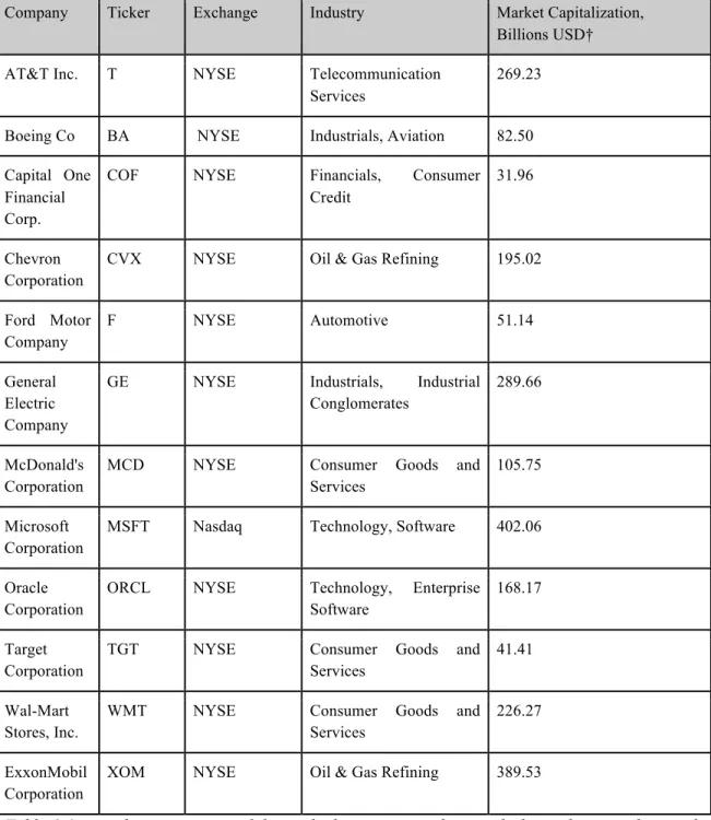
To scope the experiment, 12 companies were selected for inclusion. Each of the companies is contained within the Standard & Poor’s 500 index (“S&P500”), an internationally recognized index tracking the largest 500 companies on US exchanges. To qualify for the study, each company needed to be listed as part of the S&P500 for the duration of the experiment period.

The research uses nine years of daily trade data, beginning January 2006, ending December 2015. Model training data spans the first eight years of this 9-year period (2006 - 2014), with 2015 reserved for security forecasting. Generally, the data for each company is a matrix of 38 features by a total of 2450 observations (range 2407 to 2485, mean 2454).

To further constrain the experiment's scope and limit confounds, the companies could have no share splits or entered into major mergers with other companies during the 9-year period. Further, careful attention also was paid in company selection in an attempt to pull from a variety of economic sectors.

A full list of the companies, their sector and ticker symbol are available in Chapter 3, "Design / Methodology". The full qualification criteria are also outlined in Chapter 3, “Selection Criteria.”

1.5. Organization of Dissertation

The remainder of this dissertation is organized as follows:

● Chapter 2 ("Literature Review") is dedicated to an exploration of the previous research in security forecasting, inclusive of perspectives in finance, econometrics and machine learning. There is special attention paid to the motivation of this study's principal examination of technical indicators as inputs to security forecasting with machine learning. There is also an outline of similar studies utilizing the forecasted price as inputs to simple trading machines, which this researcher finds compelling as a model validation method.

● Chapter 3 ("Design / Methodology") will explore the selection of the participating companies in more detail. The section titled "Data Preparation" will provide details on the data transformation necessary to create valid inputs.

(15)

Subsequent sections in chapter 3 will clarify the models for both the neural network, the support vector machine and the trading algorithm used in the final evaluation phase.

● Chapter 4 ("Implementation / Results") provides a run-down of the three experimental phases applied to each of the participating company share prices. To help with data exploration, a visual guide is provided in chapter 4, section 2. Model development and model tuning are outlined in detail in Chapter 4 as well. Chapter 4 concludes with a sample of visualizations of the experiments’ results. The first section in chapter 4 ("Software") provides a detailed overview of the program developed to support the experiment and its evaluation.

● Evaluation of the experiments is reserved for Chapter 5 ("Evaluation / Analysis"). In addition to a digest of the three-phased experiments' results, observations of the experiment are provided. The limitations of this research, both of model inclusion and in rational extrapolation, are expanded in detailed in 5.3. ● Chapter 6 ("Conclusions and Future Work") provides a summary of the entire

research project, clarifies the contribution to the general body of research within security forecasting research as well as points to areas for further investigation.

(16)

2. Literature Review

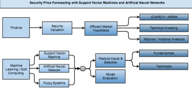
The following literature review, organized into two parts (“Finance & Econometrics” and “Machine Learning & Forecasting”) acts as a guide through a portion of the existing research into the expansive and complex field of security forecasting. There are two main topics of prior research evaluated, with Figure 1 outlining each branch:

Figure 2.1: Security Price Forecasting Landscape

Figure 2.1 provides a hierarchy of existing research used to guide the overall research question regarding the use of historical prices, and their derivatives, as valid inputs (“features”) for machine learning based security price forecasting.

First, the overarching research question is focused on exploring the validity and "rationality” of using historic prices for security forecasting and is therefore heavily influenced by previous researchers in economics, finance and behavioral psychology.

Second, the project is deeply rooted in machine learning and as such will examine previous research conducted using machine learning algorithms for security price forecasting. In particular, the Support Vector Machine (SVM) and Artificial

(17)

Neural Network (ANN) are evaluated as the primary tools for regression forecasting.

While every effort will be made to expose the historical research of each topic separately, where appropriate or unavoidable, references will be made from one topic branch to another. Perhaps somewhat outside the scope of this particular research experiment, tangentially related subtopics of research such as feature selection techniques in security forecasting will be provided to help contextualize the experiment within its general vicinity to these pre-existing soft computing applications.

As a guiding assumption, it is assumed the reader has a full understanding of the mechanics and underlying algorithmic design of SVMs and ANNs and no space in this literature review is devoted to explaining their origins or presenting their mathematical properties. An excellent primer on SVMs and ANNs is Vapnik’s The Nature of Statistical Learning Theory, Second Edition (Vapnik, 1999). In a similar manner, the forecasting of security prices is an inherently time series-based analysis. While this literature review touches upon the expansive amount of research on time series data mining techniques, a survey of best practices are available in Fu (2011) and Cao (2003).

Note on the lexicon:

In the literature, there is a varying mix of terminology for the Artificial Neural Network (ANN). Some researchers simply use the ANN while others use Multi-layer Perceptron (MLP). As far as this researcher can see, the two terms are interchangeable with some bias toward one over another, depending on application field. For the purpose of this research, ANN is used. In a similar manner, one will see a divergence in language used to describe model inputs: computer science and machine learning literature frequently use "feature" to be synonymous with "expert" whereas economics refer to "states" or “factors” and statisticians use "components". This paper uses features to denote the numerical inputs to all models. Last in this regard is a mix use of machine learning and statistical learning, which are synonymous, with differences in use typically stemming from a researcher's background in statistics (statistical learning) or computer science (machine learning). This article opts to use machine learning.

(18)

2.1. Financial Security Forecasting

As a quick reminder, this research seeks to understand what feature inputs are important and empirically legitimate for forecasting security prices. To begin to address this gap in existing computer science literature, an examination of finance and economics was in order.

2.1.1. Origins of Financial Forecasting

With such tantalizing upside, there is a considerable body of research into security price forecasting, exhibiting a wide range of creative approaches, perspectives and motivations for security exchange. Much of this research, as one might imagine, originates in finance departments, typified by efforts to seek out fundamental justification for security prices, with monikers such as arbitrage pricing theory (APT), efficient market hypothesis (EMH) and asset pricing models (Fama, 1965, 1976; Refenes, Zapranis and Francis, 1994; Ron and Ross, 1980). One might also look to game theory, in particular bargaining games, to being understanding the forces at work in the exchange of securities (Nash, 1950). Indeed, research in security forecasting also extends to evolutionary game theory (Parke and Waters, 2007). Beyond these pure economic models, there is the hotly debated method of “technical analysis” or “charting” which seeks to find patterns in historical price changes in order to ascertain future prices and market movement (Gifford, 1995; Murphy, 1999). 2.1.2. Security Valuation -- An Economist Perspective

Investigation into the economic theory of security forecasting began for this researcher with an examination of the efficient market hypothesis (EMH) due to a high-frequency of citing the EMH’s primary author Eugene Fama in machine learning literature (Fama, 1965; Fama, 1976). The EMH appeared to be one of a short list of economic models dominating the finance landscape for decades. However, despite the research of economists such as Fama showing “conclusively” that future security prices were uncoupled (“independent”) from historical prices, a school of “chartist” forecasters developed, citing Charles Dow as the principal founder due to his observation of a cyclical nature in security prices (Gifford, 1995; Bako and Sechel, 2013). Within the pursuit of identifying patterns which the cognizant investor might exploit, additional research into

(19)

the seasonality--or the predictable timing factor based on the month of the year, day of the week, etc--have also been examined. For example, Sullivan, Timmermann and White (2001) show a moderate seasonal effect. Their conclusion and evaluation of corporate need -- ie having to sell to make profits or write down losses--is compelling but they researchers clearly communicate the seasonality effects are moderate at best, further buttressing the notion that security pricing is more akin to a Random Walk (Fama, 1965; Fama and French, 1988).

Debate surrounding the validity of using charts to forecast security prices heated into the 1990s between Fama and an opposing set of economists such as DeLong, Shleifer, Summers, and Waldmann (DeLong, Shleifer, Summers, and Waldmann, 1990; Shleifer and Summers, 1990). This second group found that while “noise traders”--another pejorative name given to the investors relying upon “irrational” chart reading—may not economically possess a strong foundation, the effects of the “irrationality” on the market can be protracted, due to interaction effects with arbitrage-based investors (DeLong, Shleifer, Summers and Waldmann, 1990). Verma, Baklaci, and Soydemir (2008) even sought to understand the degree to which investor sentiment (i.e. “irrational noise”) influences stock prices. Mankiw, Romer and Shapiro (1991) cite earlier work by Shapiro showing that market volatility is indeed too high--so high, in fact, that the valuations cannot be based upon fundamental values at all.

2.1.3. Efficient Market Hypothesis and the Random Walk

To help resolve this debate, at least in the hopes of seeing justifiable input features for a security forecasting experiment, the following section examines the EMH and Random Walk in more detail.

The EMH consists of three forms: weak, semi-strong, and strong (Fama, 1970; Tsai and Hsiao, 2010). The weak form of the EMH simply examines whether future prices are a mere reflection of past prices, and in regard fall within the examination of the random walk (Fama, 1965; Fama, 1970; Tsai and Hsiao, 2010; Vui, Soon, On and Alfred, 2013). The semi-strong form of EMH posits that markets adjust rationally to publically available information such as splits, earnings announcements and adjustments to interest rates, whereas the strong form is an examination into potential monopolistic access to

(20)

information on the part of select investors or groups of investors (Fama, 1970). Despite some researchers concluding the EMH is an inaccurate depection of market behavior (Cao, Leggio and Schniederjans, 2005) or that the price movements of securities perceived to be random (in the sense of a "temporily independent random walk") is instead a noisy, non-linear process (Huang, Nakamori and Wang, 2005; Lee, 2009), machine-based security forecasting researchers frequently cite Fama's EMH (Thawornwong, Enke and Dagli, 2003; Enke and Thawornwong, 2005; Huang, Nakamori and Wang, 2005; Schulmeister, 2009; Verma, Baklaci and Soydemir, 2008; Teixeira and Inácio de Oliveira, 2010; Tsai, Hsiao, 2010; Vui, Soon, On and Alfred, 2013). This is important because under a semi-strong efficient market hypothesis, as a liberal democracy with a functionally free media and securities oversight regulatory board (such as the Securities Exchange Commission), the past prices will effectively reflect all information pertinent to the valuation of a security in the past but not in the future. Yet, many of those same researchers previously cited use historical prices to forecast future prices.

However, under the EMH, the primary inputs could be economic in nature--in a semi-strong EMH, historical prices would merely reflect all historically available information, relying upon new information to alter the base valuations. And, as such, it was here that the researcher identified one set of configurations for input features: micro- and macroeconomic factors.

2.1.4. Econometric Forecasting: (G)ARCH

Almost as a response to the EMH and its primacy as a model for security pricing, researchers began examining the evidence of what appeared to be autocorrelated events in security prices: that is, that specific patterns of price movement were followed by similar patterns, though the magnitude (positive or negative) were unknown. It was here that the Autoregressive conditional heteroscedasticity (ARCH) model, and derivatives such as generalized autoregressive conditional heteroscedasticity model (GARCH), was developed (Engle, 1982; Bollerslev, Chou, and Kroner, 1992). The ARCH model developed by Engle (1982) was proposed to forecast inflation rates in the UK and, pertinent to the EMH, depended upon past prices to arrive at the future forecast. The ARCH model was developed to help explain the clustering behavior of securities--that

(21)

large (or small) price changes will likely be followed by similarly large (or small) price changes but of an unknown sign (i.e. positive or negative) (Bollerslev, Chou, and Kroner, 1992).

The novelty of the (G)ARCH-models is that it uses a non-stationary variance--a variance in prices that changes depending on the time period evaluated within the time-series--and as such acts as a strong counter-argument to Fama’s EMH which used a (single) stable variance throughout the time-series. Because of the clustering and repetitive nature of the ARCH model, this may be a pattern intuited by technical "chartists," though that is speculation as there was no specific literature reviewed by this researcher to indicate that intuited behavior on the part of technical investors. As illustrated in the survey of ARCH and GARCH research, contemporary finance assumes that time series are continuous stochastic equations but data are typically in discrete intervals (Bollerslev, Chou and Kroner, 1992). However, this seeming gap appears to be negligible when the time series is of small enough intervals. Another appeal of ARCH-models is the ability to examine the interaction effects of various markets, macroeconomic indicators and/or securities on other markets and securities and if so to what extent because it is an inherently linear model (Bauwens, Laurent, Rombouts, 2006).

Another counter-model to the EMH, is the Autoregressive and Moving Average (ARMA) model: autoregressive (AR) and moving average (MA) (Mondal, Shit and Goswami, 2014). Autoregressive Integrated Moving Average (ARIMA) is based on ARMA Model, in which ARIMA converts non-stationary data to stationary data (ibid).

Though considerable research is conducted using the machine learning algorithms covered thus far in an effort to examine their potential improvements over (G)ARCH and ARIMA models, this is not to imply that econometric research has ceased using the aforementioned models as recent studies have shown the continued efficacy of ARIMA to forecast security prices (Mondal, Shit and Goswami, 2014; Rounaghi, Zadeh, 2016). Zhang and Frey (2015) used a combination ARMA-GARCH model for high-frequency data, though the model itself pushes the limit of linear statistical models as it uses a hidden markov to control regime switching (between ARMA and GARCH)

Despite the strong appeal of ARCH (and derivatives such as GARCH and EGARCH), the general models developed are linear in nature. The appeal of the SVM and ANN is the

(22)

ability to capture nonlinear relationships. Morefore, the process is simplified in that there is no longer a need to model variance over time. Rather than creating ever-increasing complexity to linear models, the SVM and ANN might simply skip to more elegant nonlinear models that capture the same relationships (past prices containing pertinent t+1 information) while being more comprehensible.

The important take-away for the research into (G)ARCH and ARIMA pricing models is that they do rely upon past prices as inputs, and it is here that one finds the justification for a second experimental model using historically derivative “technical” inputs to the forecasting model.

2.1.5. Investment Decisions -- A Human Behavioral Constraint

As a short primer on the behavioral economics of security forecasting, particularly in context of selecting legitimate, justifiable and rational model inputs, one must consider an examination of De Bondt and Thaler (1985) whose work in human psychological tendencies engaging in economic decision making evaluate the response of investors to information. In addition to pointing to prior work by Kahneman and Tversky work in 1982 in which they (Kahneman and Tversky) concluded that Bayes' rule is not an entirely accurate model for characterizing individual's response to the acquisition of new information, De Bondt and Thaler show that individuals tend to overweight recent information and undervalue prior, "base rate," data. In the realm of securities, this means that there is too great a discount of dividends and that stock price movements are closely tied to the changes in prior year earnings. One is left to ask, as De Bondt and Thaler do, how is it that the over-reaction to new information is a reflection of price arbitrage? The De Bondt and Thaler research fits in nicely with a vein of research into the rationality of markets with a notable mention to work conducted by Verma, Baklaci and Soydemir (2008) in which the researchers found that short-term responses are swift and severe, particularly to bad news and that the reaction extends beyond what would be rationally justified by pre-existing models. One can likely understand this intuitively but it is also backed by behavioral research conducted by Loewenstein (2000) where he states that visceral factors, those emotional states controlling preferences such as hunger, sexual drive, etc, can change rapidly because these visceral factors are themselves affected by the

(23)

changes in bodily and external stimuli. Loewenstein further concludes that it is the myriad of ever-shifting visceral states within the human which cause people who would otherwise appear “normal” to engage in extreme discounting of the future. So far as investment decisions, a discounting of the future would be an irrational mistake. For example, a “stumble” one quarter where growth was slower than expected or a merger was blocked by antitrust regulators may cause investors to “flee” irrationally, causing an unjustifiable drop in a security. This statement is also backed by Loewenstein’s (2000) investigation into decision making where he concludes that though visceral factors are transient, they can cause individuals to take extreme action and that important decisions such as investments induce powerful emotions, and as such many of life’s inflection points are heavily influenced by intense visceral states.

Friesen, Weller, and Dunham’s 2009 work plays an important role in the further investigation of trading rules as well as the role of confirmation bias, particularly in light of bias, autocorrelation and the justification for interpreting the past to posit the future. Friesen, Weller, and Dunham find there is indeed indication of momentum in stock prices over the short-term, which provides the evidence to support trading rules designed to detect these short-term trends. Aligning well again with the work from Verma et al. (2008), the researchers point to large, infrequent signals (market news including economic changes) as rationally interpreted while shorter-term, higher-frequency signals (war, supply constraints) may be interpreted in a biased manner.

While economists frequently characterize the actors within the economy as rational, with investors lauded as a special class within the general body of economic actors, this may be an oversimplification. Fama himself stated that his finance models assumed actors assessed the universe of alternatives but that, “[it is] completely unrealistic to presume that when market prices are determined, they result from a conscious assessment...by all or even most or even many investors” (Fama, 1976).

So, when one uses machine learning to forecast prices, the machine algorithms base their learning in historical reactions (by individuals) to new market stimuli. It is for this purpose, the third set of experimental inputs consists of a blend of purely technical and purely fundamental inputs is formed. In a sense, it becomes a question of whether the

(24)

machine algorithms effectively “learn” how individuals might respond to both historical patterns (technicals) and the change in economic conditions (fundamentals).

2.2. Machine Learning and Forecasting

The forecasting problem, due to the constant variability of prices and the differing motivations of the actors prompting these exchanges, constitutes non-trivial knowledge discovery (Fayyad, Piatetsky-Shapiro and Smyth, 1996). As such, the data mining and machine learning research communities were quick to pick up the mantel of examining the nonlinear problem of price changes with over two decades of research into a variety of nuanced approaches (Atsalakis and Valavanis, 2009; Vui et al., 2013). Beyond simply security prices, machine learning has been applied to other nonlinear problems, including wind forecasting, sunspot location, bankruptcy candidates and corporate (financial) distress (Liu, Tian, and Li, 2012; Cao, 2003; Tsai, 2009; Li, Wang, and Chen,2015). 2.2.1. Artificial Neural Networks

Beginning in the early 1990s, researchers focused on comparisons of neural networks with traditional statistical approaches, allured by the ability to provide better forecasting under non-parametric conditions (Wang, Wang, Zhang, and Guo, 2011). As one might expect, researchers began by trying to show the power of advanced algorithms such as the Artificial Neural Network (ANN) to outperform generally established forecasting benchmarks such as [Generalized] Autoregressive Conditional Heteroskedasticity ([G]ARCH) (Refenes, Zapranis and Francis, 1994; Guresen, Kayakutlu, and Daim, 2011). After a flurry of research with ANN designs ranging from Multi-Layer Perceptron (MLP) with general forward feed (FF-NN) (Refenes, Zapranis and Francis, 1994; Atsalakis and Valavanis, 2009) and slightly more complex backpropagation (BP-NN) (Wang, Wang, Zhang, and Guo, 2011), the field saw further innovation and advancement with a myriad of different flavors of backpropagation error-regulating algorithms ranging from Bayesian regulators (Ticknor, 2013) to artificial bee colonies (Hsieha, Hsiao, and Yeh, 2011) to genetic algorithm (GA) (Wang et al., 2012). Results with ANN have been consistently promising but the improved forecasting with advanced machine algorithms such as ANN and GA should not be used to conclude the models do not rely upon the assumption of

(25)

linear correlations as previous statistical models do (Wang et al., 2012). According to the survey work conducted by Vui, Soon, On and Alfred (2013), the forward feed neural network (FF-NN) is most common and outperforms probabilistic ANN (though not conclusively), with strong evidence also pointing to the viability of genetic algorithms for the backpropagation (BP) portion of a BP-NN.

2.2.2. Support Vector Machines

In tandem to the work with ANN, data mining and machine learning researchers began applying other algorithms to the nonlinear problem, including Support Vector Machines (SVM), now a mainstay in contemporary machine algorithm research (Tay and Cao, 2001; Huang, Nakamori and Wang, 2005; Li, Wang and Chen, 2015). The primary difference between the SVM and the ANN is the optimization strategy. Whereas the ANN seeks to minimize the (empirical) error rate and find a global minimum, the SVM seeks to reduce structural risk, minimizing an upper bound of generalization and so is, by its nature, less prone to being “stuck” in a local minimum (Cao, 2003; Tay and Cao, 2005; Lee, 2009; Wen, Yang, Song, and Jia, 2010; Chai, Du, Lai, and Lee, 2015; Li, Wang and Chen, 2015).

Researchers have also lauded the simplicity of the algorithm itself, which has fewer parameters to concern researchers, unlike an ANN which worries about depth and breadth of architecture as well as learning rates and penalty weights (Refenes, Zapranis and Francis, 1994; Cao, 2003; Kara, Boyacioglu and Baykan, 2011; Vui, Soon, On and Alfred, 2013).

2.2.3. Fuzzy Logic

While some research may be mired in an attempt to forecast the market exactly, a fuzzy logic approach seeks to simplify the problem. Some researchers simply choose to forecast the direction of the market (Kim, 2003; Lee, 2009; Huang, Nakamori, and Wang, 2005; Kara, Boyacioglu and Baykan, 2011) while others have created simple algorithmic rules for buying and selling securities (Kim and Han, 2001; Thawornwong, Enke, and Dagli, 2003; Enke, Thawornwong, 2005; Teixeira and Inácio de Oliveira, 2010; Chang, Fan and Lin, 2011).

(26)

Despite the depth of literature available for the evaluation of ANNs applied to forecasting, one should not conclude the ANN is the out-right best model. Indeed, the SVM model constructed by Ni, Ni and Gao (2011) was provacoative while the trading system constructed by Teixeira, L.A. and Inácio de Oliveira (2010) relied upon the Nearest Neighbor algorithm and performed well, relative to general literature benchmarks which used profit comparisions to “buy and hold” strategies. Further, the fuzzy rule model proposed by Kim and Han (2001) did not rely on any advanced algorithms for making trading decisions, instead constructed simple buy-, sell-, and hold-conditions (i.e. simple “if-then-else” clauses) and also showed promising results.

There is a strong affinity between “fuzzy” logic and security forecasting because of the volatile and imprecise nature of security prices. By generalizing away from the specifics of an exact price and focusing model development on general trends (such as gain or loss), researchers are better equipped to make significant progress without burdening themselves with the need to find the “single true model,” which may not exist for all securities. To provide a concrete example, the researchers Enke and Thawornwong (2005) constructed a novel trading algorithm for purchasing the S&P500 or 10-year Treasury Bills. The inputs to the system relied upon fundamental variables and fed into an ANN. They found the trading system was able to outperform against simple Buy-and-Hold strategies. Nonetheless, the authors were also careful to point out that better performance does not necessarily equate to being more profitable as asset allocation is of paramount importance with investment decisions.

The paradigm of using fuzzy logic rules or fuzzy models plays a large role in the design of the overall experiment, in particular the development of a buy-sell machine to make comparisons to “buy-and-hold” strategies. For this researcher, the use of fuzzy systems to operationalize the forecasts of a precise machine algorithm, be that ANN or SVM, is exceptionally compelling because the fuzzy system is able to step outside traditional statistical metrics for something more tangible: profit or loss.

2.2.4. Feature Selection and Inputs for Machine Algorithms

When approaching a machine learning problem, an important decision to make is what feature inputs are relevant to solving the problem--as the saying goes, “garbage in,

(27)

garbage out.” In fact, the very motivation of the research question herein is to locate legitimate, rational and justifiable model inputs.

In the literature there is an expansive set of inputs employed. Atsalakis and Valavanis (2009) summarize the results showing a huge diversity of inputs, not just with a simple dichotomy of “technical versus fundamental indicators” but with a large diversity within those selections, too. For security forecasting, understanding the difference and role of fundamental and technical indicators appears to be a key issue.

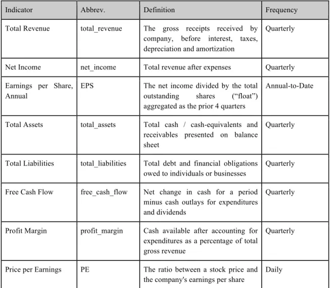
Whereas fundamental factors are the macro- and microeconomic restrictions to a business (interest rates, cash flow, product margins, dividends, and general costs of doing business), technical indicators are values derived from historical trade information, such as Open and Close prices and total volume of securities exchanged (Fama, 1976; Shleifer and Summers, 1990; Gifford, 1995; Murphy, 1999; Tsai and Hsiao, 2010). Of note is that many of the features described as “fundamentals” might equally be classified as technicals--volume is an interesting example, frequently cited as a fundamental under the justification of it representing one of the economic conditions under which a security is traded (Ticknor, 2013). Volume, as a proxy indicator for the Efficient Market Hypothesis, appears to be a stretch of the definition. For the purposes of our evaluation, we will make a clear delineation between economic factors such as interest rates, currency exchanges and natural gas prices as fundamentals and volume and price or price derivatives (Moving Average, Relative Strength Indicator) as technical features.

One method to resolve the input problem by researchers is simply to aggregate a large set of feature inputs, ranging from variously derived technical values to a selection of economic fundamentals, and then to implement feature reduction. Stepwise Regression Analysis is one such technique, as implemented by Chang, Fan, and Lin (2011). Principal Component Analysis (PCA) is another common selection (Tsai, and Hsiao, 2010).

Tsai and Hsiao (2010) took a creative approach of applying a pseudo-ensemble of three feature reduction techniques, PCA, GA and Classification and Regression Trees (CART), and applying them as single model evaluations, “joins” and “intersects” of selected features, ultimately concluding that an intersection of selected features between PCA and GA as inputs to a BP-ANN provided the best results while GA was the most effective of the individual feature reduction techniques in their model.

(28)

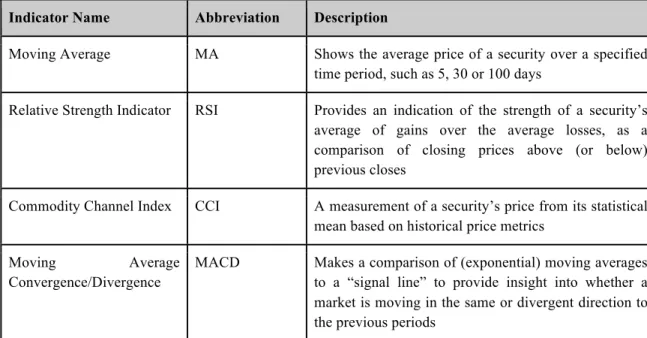
The literature appears to be predominantly comprised of technical input variables, particularly derivatives values such as Simple Moving Average (and variations), Commodity Channel Index and Moving Average Convergence Divergence (MACD), to name but a few. It’s unclear if this is a conscious choice over the selection of fundamentals as the motivation for selecting one set of inputs over another is not frequently explored in detail, if at all. Notable exceptions to this are Thawornwong, Enke and Dagli (2003) and Enke and Thawornwong (2005) who in the two studies, exclusively examined the role of technicals and fundamentals (respectively) on price forecasting. Nonetheless, the choice of technicals almost implies the “noise trader” approach as a bias, since technicals use historical price data to establish a pattern. That is, the technical variables themselves are derivatives of the price movements over time, establishing to some degree a picture of momentum--Momentum and Moving Average being two commonly used technical indicators. Table 2.1 provides a small example of the technical variables used as inputs into both traditional statistical and machine algorithm based models.

Indicator Name Abbreviation Description

Moving Average MA Shows the average price of a security over a specified time period, such as 5, 30 or 100 days

Relative Strength Indicator RSI Provides an indication of the strength of a security’s average of gains over the average losses, as a comparison of closing prices above (or below) previous closes

Commodity Channel Index CCI A measurement of a security’s price from its statistical mean based on historical price metrics

Moving Average

Convergence/Divergence

MACD Makes a comparison of (exponential) moving averages to a “signal line” to provide insight into whether a market is moving in the same or divergent direction to the previous periods

Table 2.1 provides a small example of historically derivative metrics used both by investment practitioners and machine learning researchers as feature inputs to their models.

(29)

While much of the existing literature reviewed here focuses on the use of technical indicators as proxies for available information -- that is, as a method of expressing the Efficient Market Hypothesis -- there are no reviewed models relying upon the daily news as a component of feature inputs. Indeed, with the findings from Verma et al. (2008) indicating the at-times voraciously salient impact of sentiment on security prices, one would expect a set of sentiment analyses to be more routine. One interesting model which does make use of text mining techniques (of company management’s “discussions” within quarterly and annual reports) as an input to security forecast is presented by Wang, Huang and Wang (2012). Their text mining approaches improved the predictive efficacy of a traditional Autoregressive Interval Moving Average (ARIMA) model.

2.2.5. The “What” of Security Forecasting

When evaluating the securities forecasting literature, it becomes evident that many researchers chose, rather than specific company share prices, to forecast stock indicies such as the Dow Jones Industrial Average (DJIA) (Wang, Wang, Zhang and Guo, 2011), the S&P 500 (S&P), the London FTSE 100 (Hsieh, Hsiao and Yeh, 2011) and emerging

market indices including the Sao Palo Stock Exchange (SPSE) (Teixeira and Inácio de Oliveira, 2010) and the Istanbul Stock Exchange (ISE) (Kara, Boyacioglu and Baykan, 2011). Perhaps it is simply precedent as much of the early research was done in this regard. However, there are some researchers who focused on specific shares for their forecasting (Thawornwong, Enke and Dagli, 2003). Others yet, create a basket of shares in order to approximate indices (Guresen, Kayakutlu and Daim, 2011), the index itself or even significantly large portions of the index component shares (Huang, Nakamori and Wang, 2005; Wen, Yang, Song and Jia, 2010).

When reading research on the forecasting of an index, one has to wonder why the index was chosen--this reason and motivation for the selection of an index goes frequently unstated, leaving one only to speculate: perhaps the index has a smoothing effect, allowing the researchers to more easily apply a model in a pre-generalized method with a built-in bias for momentum where the aggregate “herd” of stocks moves cohesively, thereby lending itself well to the machine learning algorithms. Moreover, the studies forecasting the index often seek to forecast the direction of the index (Kim, 2003) and so are able to

(30)

report significantly higher accuracy rates, even though the base rate for a boolean is essentially 50% (under “random” conditions).

In this manner, one is left to suspect some form bias, perhaps even unconscious, but nonetheless providing ground for Keogh and Kasetty’s (2003) call for better benchmarking in data mining: choosing test candidates that will create more impactful model results than if applied to a more complex scenario. To balance the last statement, one should note the challenges of forecasting a specific value for a single time observation when the ratio of signal-to-noise is low and so directional prediction is an arguably valid simplification mechanism. Others have sought to forecast the probability distributions of an index-at-close as another simplification process (Weigend and Shi, 2000).

2.2.6. Data Pre-Processing

Not to be confused with the somewhat pejorative moniker “noise trader,” an emerging body of research now takes to applying wavelet algorithms to the price inputs in an attempt to “denoise” the variable inputs. An early example of pre-training data transformation is Tay and Cao (2001) in which they transformed the prices into a relative difference in percentage of price, which makes the data more symmetrical. After this transformation, the authors went a step further by replacing all values that were more than two standard deviations with the next closest value. The goal with the replacements was to remove the major shocks in the learning algorithm's training set, under the presumption that those events were rare and simply added to the overall noise in the system. This transformation was unique to the reviewed literature but might be considered a precursor, in some ways, to future wavelet transformations which sought to reduce noise and variance by applying smoothing functions.

Hsieh, Hsiao and Yeh (2011), for example, applied the Haar wavelet transform to decompose the price feature before conducting stepwise regression analysis for feature selection--their model ultimately fed into an artificial bee colony-driven BP-ANN. Another compelling example of wavelet transforms applied to price inputs was conducted by Wang, Wang, Zhang and Guo (2011) in which a threefold Discrete Fourier Transform (DFT) was applied, in an attempt at separating the noise from the signal. In this study,

(31)

Wang et al. found two passes with the DFT into a ANN outperformed the third transformation pass, in which too much signal flattening had occurred.

Another common pre-processing step is to normalize the feature values so that they range from 0 to 1 or -1 to 1 (Lee, 2009; Wen, Yang, Song, and Jia, 2010). This is done so that none of the features carry too large a weight. That is, if a feature input such as Volume is used, it may be measured in millions of units but another input feature such as a moving average may only be measured in tens (or hundreds) or dollars.

2.2.7. Ensembles: Multiple Predictors are Greater than One

A theme noteworthy within the literature is the inclusion of ensembles. An ensemble is the combination of multiple prediction models or model pipelines combined, often through a weighting or ‘voting’ mechanism, that through the blending of the forecasts, is able to make better predictions. (Dietterich, 2000) The rational thought exercise leading to an ensemble technique is that if there is a complex task for which a learning expertise is required to perform, then multiple experts will perform better than one. (Huang, Nakamori and Wang, 2005) Bagging, an ensembling technique, takes different samples from the overall training set (with replacement for each removed sample) and uses these subsets as inputs to the learning algorithm. The outputs are then blended to arrive at a final model prediction. (West, Dellana and Qian, 2005) Another ensembling technique Adaptive Boosting (or ‘AdaBoosting’ or, simply, ‘Boosting) is an iterative, resampling technique in which the misclassified classes are given a higher distribution in the new sample, and correctly classified are given a lower distribution. (West, Dellana and Qian, 2005) After the resample is complete, the algorithms are retrained and new forecasts provided. This process may be completed multiple times.

While there is some evidence of ensemble in the literature, ensembling does not appear as a standard technique, rather a single "best model" is still the frequent reporting tool. This may not necessarily be due to researcher bias but simply the result of a complex field still seeking to homogenize around general single-model best practices. It was the reliance upon a single model which motivated West, Dellana and Qian (2005) to evaluate cross-validation, bagging and boosting as possible ensemble techniques--ultimately concluding that an ensemble of ANN models outperformed the single best model.

(32)

Examples of ensembles in security forecasting literature include Huang, Nakamori, and Wang (2005), Tsai and Hsiao (2010), Wang, Wang, Zhang, and Guo (2012), Wang, Wang, Zhang, and Guo (2011), and Wu, Luo and Li (2015).

When implementing ensembling techniques, experimenters should be wary of the findings from Zhou, Wu and Tang (2002) who found that ensembling some (or many) of the predicted models may perform better than an across-the-board aggregation of all models, particularly when measuring for a generalized model.

2.2.8. Model Evaluation

The last major research area pertinent to this experiment is the method of model evaluation. As Keogh and Kasetty (2003) illustrate, there is a need for creating a rigorous method of evaluating a model’s efficacy, an area according to Keogh and Kasetty (ibid) the data mining community has been prone to positing exaggerated results. Despite a lack of clear-cut benchmarks, the literature for model evaluation is as diverse as the predictive models.

In terms of statistical measures, many researchers chose to use measures such as root mean square error (RMSE) (Kara, Boyacioglu and Baykan, 2011), mean absolute percent error (MAPE) (Ticknor, 2013), mean squared error (MSE) (Wen, Yang, Song, and Jia, 2010) and normalized mean square error (Tay and Cao, 2002). As stated previously, some researchers elected to forecast the direction of the market--for example whether the next day movement of the market will be higher or lower than the previous day. In these instances, the researchers chose classification metrics such as F1 scores (Lee, 2009). Others yet chose to compare their models based on profitabilty (Kim and Han, 2001; Thawornwong, Enke and Dagli, 2003; Teixeira and Inácio de Oliveira, 2010; Wen, Yang, Song and Jia, 2010) and in some cases developing trading algorithms for comparision with the less active investement strategy of “buying and holding” (Kim and Han, 2001; Thawornwong, Enke and Dagli, 2003; Enke and Thawornwong, 2005). From a the 100-plus survey conducted by Atsalakis and Valavanis (2009), it is clear that researchers use varying evaluation techniques for their models. However, the standard statistical measures are used, namely root mean square error (RMSE), mean absolute error (MAE) and mean squared error (MSE), with perhaps a skew toward using RMSE. One advantage of RMSE

(33)

is that the results are reported in the same form as the predicted variable--for example “dollars” for a stock price.

As one might expect, there is a mixed set of results regarding the comparison of various algorithmic approaches to security forecasting, with some researchers claiming outperformance with SVMs while others illustrate "conclusively" the superior efficacy of ANNs (Huang, Nakamori and Wang, 2005; Kara, Boyacioglu, and Baykan, 2011). Moverover, the detailed meta-study of over 100 research studies, many of which included internal comparisons themselves, conducted by Atsalakis and Valavanis (2009) did not conclude with a single-best model archetype, but the rather conservative notion that ANN and neuro-fuzzy models are appropriate soft computing techniques for stock forecasting.

2.3. Summary

2.3.1. Summary of Literature

A common thread in security forecasting model inputs is a citation of Fama's Efficient Market Hypothesis (EMH), which effectively states that an efficient market is one in which information freely disseminates and is therefore fully reflected in a security price (Fama, 1965; Fama, 1970; Cao, Leggio and Schniederjans, 2005). That is, security prices fully reflect all public information pertinent to a security, with no information “advantage” that some arbitrage investors have over others. The market is informationally efficient and so security prices fully reflect all information. As such, the use of historical prices to forecast future prices is invalid because it is only new information not reflected in security prices (new innovations, new market growth, new profitability, etc) that will impact future prices. Nonetheless, there are dozens and dozens of studies which rely upon technical indicators to forecast the future—and claims of successfully doing so while citing the Efficient Market Hypothesis as relevant.

2.3.2. Gaps in Literature and Open Problems

So perhaps ironically, these researchers cite the EMH from an act of precedent in prior influential work but then use tools which would seemingly contradict the EMH. In any case, one is left to ask, “are technical values reliably useful as inputs to a security

(34)

Figure