Bayesian non-parametric conditional copula estimation of twin data

(1)

Kent Academic Repository

Full text document (pdf)

Copyright & reuse

Content in the Kent Academic Repository is made available for research purposes. Unless otherwise stated all content is protected by copyright and in the absence of an open licence (eg Creative Commons), permissions for further reuse of content should be sought from the publisher, author or other copyright holder.

Versions of research

The version in the Kent Academic Repository may differ from the final published version.

Users are advised to check http://kar.kent.ac.uk for the status of the paper. Users should always cite the published version of record.

Enquiries

For any further enquiries regarding the licence status of this document, please contact: [email protected]

If you believe this document infringes copyright then please contact the KAR admin team with the take-down information provided at http://kar.kent.ac.uk/contact.html

Citation for published version

Dalla Valle, Luciana and Leisen, Fabrizio and Rossini, Luca (2018) Bayesian non-parametric

conditional copula estimation of twin data. Journal of the Royal Statistical Society: Series C

(Applied Statistics), 67 . pp. 523-548. ISSN 0035-9254.

DOI

https://doi.org/10.1111/rssc.12237

Link to record in KAR

http://kar.kent.ac.uk/62861/

Document Version

Publisher pdf

(2)

_{2017 The Authors Journal of the Royal Statistical Society: Series C (Applied Statistics)} Published by John Wiley & Sons Ltd on behalf of the Royal Statistical Society.

This is an open access article under the terms of the Creative Commons Attribution-NonCommercial License, which permits use, distribution and reproduction in any medium, provided the original work is properly cited and is not used for commercial purposes.

0035–9254/18/67523

Appl. Statist.(2018)

67,Part3,pp.523–548

Bayesian non-parametric conditional copula

estimation of twin data

Luciana Dalla Valle, University of Plymouth, UK Fabrizio Leisen

University of Kent, Canterbury, UK and Luca Rossini

Ca’ Foscari University of Venice and Free University of Bozen-Bolzano, Italy

[Received March 2016. Final revision June 2017]

Summary.Several studies on heritability in twins aim at understanding the different contribution of environmental and genetic factors to specific traits. Considering the national merit twin study, our purpose is to analyse correctly the influence of socio-economic status on the relationship between twins’ cognitive abilities. Our methodology is based on conditional copulas, which enable us to model the effect of a covariate driving the strength of dependence between the main variables. We propose a flexible Bayesian non-parametric approach for the estimation of conditional copulas, which can model any conditional copula density. Our methodology extends the work of Wu, Wang and Walker in 2015 by introducing dependence from a covariate in an infinite mixture model. Our results suggest that environmental factors are more influential in families with lower socio-economic position.

Keywords: Bayesian non-parametrics; Conditional copula models; National merit twin study;

Slice sampling; Social science

1. Introduction

The literature on heritability of traits in children often focuses on twins, because of the shared environmental factors and the association of genetical characteristics. Among studies on the

heritability of diseases, Wanget al.(2011) applied an efficient estimation method to mixed effect

models to analyse disease inheritance in twins.

One of the main purposes of studies on heritability is to estimate the different contribution of genetic and environmental factors to traits or outcomes (see, for example, the latent class twin

method of Baker (2016)). Bateset al.(2013) studied the interactions between environmental

and genetic effects on intelligence in twins, showing that higher socio-economic status is as-sociated with higher intelligence scores. Bioecological theory states that environmental factors may significantly influence the heritability of certain characteristics, such as cognitive ability, which is the readiness for future intellectual or educational pursuits. Several studies have found that cognitive ability is more pronounced and evident among children who are raised in higher socio-economic status families. Such families can offer greater opportunities to children, due Address for correspondence: Fabrizio Leisen, School of Mathematics, Statistics and Actuarial Sciences, Corn-wallis Building, University of Kent, Canterbury, Kent, CT2 7NF, UK.

(3)

to their socio-economic wealth status, and represent stimulating environments where children’s inherited capabilities may become more manifest.

The aim of this paper is to analyse correctly the effect of socio-economic factors on the relationship between twins’ cognitive abilities. From a sample of 839 US adolescent twin pairs who completed the national merit scholarship qualifying test (NMSQT), we consider each twin’s overall school performance (measured by a total score including English, mathematics, social science, natural science and word usage), the mother’s and father’s education level and the family income. The data are plotted in Fig. 1, which shows the scatter plots of the twins’ school performances, on each axis, against the socio-economic variables, whose values are in different colours (dark denotes low values, whereas light denotes high values). Fig. 1 indicates that the twins’ school performances are positively correlated and their dependence is influenced by the values of the socio-economic variables (the mother’s (Fig. 1(a)) and the father’s level of education (Fig. 1(b)) and the family income (Fig. 1(c))). Indeed, most of the light dots (denoting high values of the covariates) are grouped in the upper right-hand corner, whereas the dark dots (denoting low values of the covariates) lie in the bottom left-hand corner of each plot. Hence, the higher the parents’ education or family income, the higher is the twins’ school performance. This means that the twins’ performance scores are functions of each covariate and they vary according to the values of the covariates.

Selection score (total) first twin 20 40 60 80 100 120 140 160 180

Selection score (total) second twin 0

1 2 3 4 5 6

Mother‘s level of education

(a)

Selection score (total) first twin 20 40 60 80 100 120 140 160 180

1 2 3 4 5 6

Father‘s level of education

(b)

20 40 60 80 100 120 140 160 20 40 60 80 100 120 140 160

20 40 60 80 100 120 140 160 Selection score (total) first twin 20 40 60 80 100 120 140 160 180

1 2 3 4 5 6 7 Family‘s income (c)

Fig. 1. Scatter plots of the twins overall scores with respect to (a) the mother’s and (b) father’s level of education and (c) family income

(4)

Copula Estimation of Twin Data 525

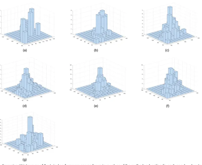
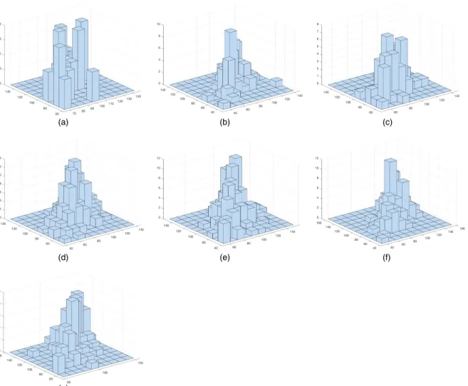
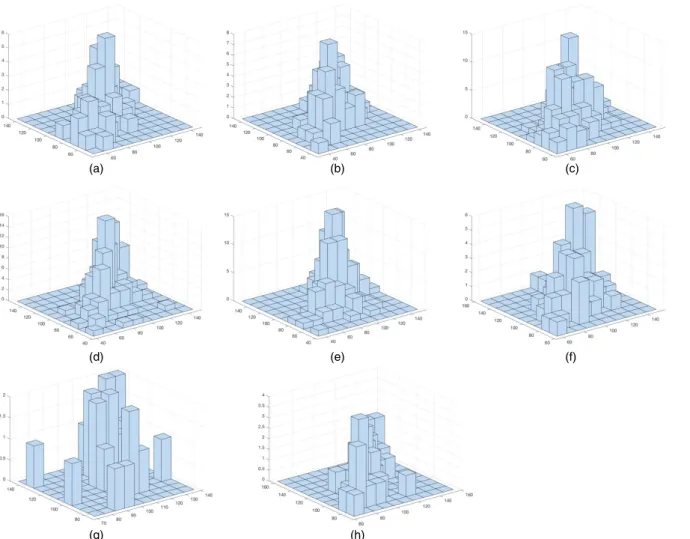
In Fig. 2 we produced three-dimensional histograms of the twins’ performance scores for various values of the mother’s education. Similar plots for the father’s level of education and family income are included in Figs 3 and 4. The different shapes of the histograms corresponding to different levels of the covariates suggest that the dependence structure between the twins’ school outcomes changes according to the values of the mother’s and father’s education and family income. Therefore, a flexible model, which can capture the effect of a covariate on the dependence between the children’s performance scores, is necessary.

To model the dependence structure between the twins’ school performances, we use copulas, which are popular modelling approaches in multivariate statistics allowing the separation of the marginal components of a joint distribution from its dependence structure. More precisely,

Sklar (1959) proved that ad-dimensional distributionHof the random variablesY1,: : :,Ydcan

be fully described by its marginal distributions and a functionC: [0, 1]d_→_{[0, 1], called a copula,}

through the relationH.y1,: : :,yd/=C{F1.y1/,: : :,Fd.yd/}. In the literature, copulas have been

applied to model the dependence between variables in a wide variety of fields (see Kolevet al.

(2006) and Cherubiniet al.(2004)). In particular, applications of copula models have involved

lifetime data analysis (Andersen, 2005), survival analysis of Atlantic halibut (Braekers and Veraverbeke, 2005) and transfusion-related acquired immune deficiency syndrome and cancer

analysis (Emura and Wang, 2012; Huang and Zhang, 2008; Owzaret al., 2007).

The introduction of covariate adjustments to copulas has attracted increased interest in recent years. Craiu and Sabeti (2012) proposed a conditional copula approach in regression settings where the bivariate outcome can be continuous or mixed. Patton (2006) introduced time vari-ation in the dependence structure of auto-regressive moving average models (see also Jondeau

and Rockinger (2006) and Bartramet al.(2007) for other applications of time series analysis to

dependence modelling). Acaret al.(2010) provided a non-parametric procedure to estimate the

functional relationship between copula parameters and covariates, showing that the gestational

age drives the strength of dependence between the birth weights of twins. Abegazet al.(2012)

and Gijbelset al.(2012) proposed semiparametric and non-parametric methodologies for the

estimation of conditional copulas, establishing consistency and asymptotic normality results for the estimators. The methodology is then applied to examine the influence of the gross domestic

product, in US dollarsper capita, on the life expectancy of males and females at birth.

In a similar vein, parametric models such as Bayesian regression copulas allow the specifica-tion of Bayesian marginal regressions for a set of outcomes, linking the marginals to covariates, and combining them via a copula to form a joint model. The general framework of Bayesian Gaussian regression copulas with discrete, continuous or mixed outcomes was presented by Pitt et al.(2006) and enables handling a multivariate regression with Gaussian and non-Gaussian marginal distributions.

Yin and Yuan (2009) adopted a Bayesian regression copula model in cancer clinical trials for dose finding to account for the synergistic effect of combinations of multiple drugs. A

cop-ula constructed from the skewt-distribution was employed by Smithet al.(2012) to capture

asymmetric and extreme dependence between variables modelled via Bayesian marginal regres-sions. Whereas most Bayesian regression copula models focus on covariate adjustments for the marginals, recently Klein and Kneiss (2016) proposed simultaneous Bayesian inference for both the marginal distributions and the copula. Other contributions along the same lines are

Taglioniet al.(2016) and Standeret al.(2015a,b). However, Klein and Kneiss (2016), Taglioni

et al. (2016) and Standeret al. (2015a,b) selected the copula family by using the deviance in-formation criterion, which may suffer from limitations, as discussed for example by Plummer (2008). Indeed, the choice of the copula family may be controversial and it is still an open problem (see Joe (2014)). The literature offers a rich range of copula families, such as elliptical

(5)

L. Dalla V alle, F. Leisen and L. Rossini (a) (b) (c) (d) (e) (f) (g)

Fig. 2. Three-dimensional histograms of the twins’ performance scores for various values of the mother’s education (in each panel,xdenotes the level of

the covariate andnxdenotes the relevant sample size): (a)xD0,n0D19; (b)xD1,n1D54; (c)xD2,n2D105; (d)xD3,n3D305; (e)xD4,n4D195; (f)

(6)

Copula Estimation of T win Data 527 (a) (b) (c) (d) (e) (g) (f)

Fig. 3. Three-dimensional histograms of the twins’ performance scores for various values of the father’s education (in each panelxdenotes the level of

the covariate andnxdenotes the relevant sample size): (a)xD0,n0D24; (b)xD1,n1D90; (c)xD2,n2D98; (d)xD3,n3D212; (e)xD4,n4D178; (f)

(7)

L. Dalla V alle, F. Leisen and L. Rossini (a) (b) (c) (d) (e) (f) (g) (h)

Fig. 4. Three-dimensional histograms of the twins’ performance scores for various values of family income (in each panelx denotes the level of the

covariate andnxdenotes the relevant sample size): (a)xD0,n0D62; (b)xD1,n1D92; (c)xD2,n2D200; (d)xD3,n3D166; (e)xD4,n4D183; (f)xD5,

(8)

copulas (e.g. Gaussian and Student’st) and Archimedean copulas (e.g. Frank, Gumbel,

Clay-ton and Joe copulas) to accommodate various dependence structures. In this paper, we adopt a Bayesian non-parametric approach which enables us to overcome the issue of the choice of copula and we adopt a conditional copula approach to model the effect of a covariate on the

dependence between variables. Our methodology builds on Wu et al.(2015), who proposed

a Bayesian non-parametric procedure to estimate any unconditional copula density function. They combined the well-known Gaussian copula density with the modelling flexibility of the Bayesian non-parametric approach, proposing to use an infinite mixture of Gaussian copulas. Burda and Prokhorov (2014) proposed to use non-parametric univariate Gaussian mixtures for the marginals and a multivariate random Bernstein polynomial copula for the link

func-tion under the Dirichlet process prior. Our paper extends the work of Wuet al.(2015) to the

conditional copula setting, by proposing a novel methodology which combines the advantages of a conditional copula approach with the modelling flexibility of Bayesian non-parametrics. In particular, we include a conditional covariate component to explain the variable depen-dence structure, allowing us further flexibility to the copula density modelling. To the best of our knowledge, this is the first Bayesian non-parametric proposal in the conditional copulas literature.

The outline of the paper is as follows. In Section 2 we briefly review the literature about con-ditional copulas and Bayesian non-parametric copula estimation. In Section 3 we introduce our novel Bayesian non-parametric conditional copula setting. Section 4 provides an algorithm for estimating the posterior parameters and Section 5 illustrates the performance of the methodol-ogy. Section 6 is devoted to the application of our methodology to the analysis of the national merit twin study. Concluding remarks are given in Section 7.

The code that was used to analyse the data can be obtained from http://wileyonlinelibrary.com/journal/rss-datasets

2. Preliminaries

In this section, we review some preliminary notions about conditional copulas and illustrate the

Bayesian non-parametric copula density estimation that was introduced in Wuet al.(2015). In

what follows, we focus on the bivariate case for simplicity; however, the arguments can be easily extended to more than two dimensions.

2.1. The conditional copula

Let Y1 andY2 be continuous variables of interest andX be a covariate that may affect the

dependence betweenY1andY2. Following Gijbelset al.(2012), Abegazet al.(2012) and Acar

et al.(2010), we suppose that the conditional distribution of.Y₁,Y₂/givenX=xexists and we denote the corresponding conditional joint distribution function by

Hx.y1,y2/=P.Y1y1,Y2y2|X=x/:

If the marginals ofHx, denoted as

F_1x.y₁/=P.Y₁y₁|X=x/, F2x.y2/=P.Y2y2|X=x/,

(9)

Cx.u,v/=Hx{F_1x−1.u/,F_2x−1.v/} .1/

where F_1x−1.u/=inf{y₁:F_1xu} andF_2x−1.v/=inf{y₂:F_2xv} are the conditional quantile

functions and u=F_1x.y₁/ and v=F_2x.y₂/ are called pseudo-observations. The conditional

copula Cx fully describes the conditional dependence structure of.Y1,Y2/ given X=x. An

alternative expression for copula (1) is

Hx.y1,y2/=Cx{F1x.y1/,F2x.y2/}: .2/

2.2. Bayesian non-parametric copula density estimation

LetΦρ.y1,y2/denote the standard bivariate normal distribution function with correlation

co-efficientρ. Then,Cρis the copula corresponding toΦρ, taking the form

Cρ.u,v/=Φρ{Φ−1.u/,Φ−1.v/} .3/

whereΦis the univariate standard normal distribution function. The Gaussian copula density

is cρ.u,v/= |Σ|−1=2exp −1 2.Φ −1_.u/_,_Φ−1_.v//._Σ−1₋_I_/Φ−1.u/ Φ−1.v/ .4/ where the correlation matrix is

Σ= 1 ρ ρ 1 :

Wuet al.(2015) proposed to use an infinite mixture of Gaussian copulas for the estimation of a copula density, as follows:

c.u,v/= ∞ j=1

wjcρj.u,v/ .5/

where the weights wj sum to 1 and the ρjs vary in .−1, 1/. Given a set of n observations

.u₁,v₁/,: : :,.un,vn/, their model can be described through a hierarchical specification, i.e. .ui,vi/|ρi ind ∼cρi.ui,vi/, i=1,: : :,n, ρi|G IID ∼G, G∼DP.λ,G₀/, .6/

whereGis a Dirichlet process prior with total massλand base measureG₀. This proposal is

motivated by the fact that bivariate density functions on the real plane can be arbitrarily well approximated by a mixture of a countably infinite number of bivariate normal distributions of the form f.y₁,y₂/= ∞ j=1 wjN{.y1,y2/|.µ1j,µ2j/,Σj}

whereN{.y1,y2/|.µ1j,µ2j/,Σj}is the joint bivariate normal density with mean vector.µ1j,µ2j/

and correlation matrixΣj(see Lo (1984) and Ferguson (1983)). Roughly speaking, Lo (1984)

and Ferguson (1983) are mimicking the Dirichlet process mixture model in the copula setting (see Escobar (1994) and Escobar and West (1995)). The sampling strategy follows the slice

sampler of Walker (2007) and Kalliet al. (2011), who showed that the Gaussian mixture is

(10)

3. Conditional copula estimation with Dirichlet process priors

The data object of study requires a model which can take into account the effect of a covariate. We

build on the model that was introduced by Wuet al.(2015) and illustrated in the previous section.

The idea is to replace the Gaussian copula with a conditional version where the correlation is a function of the covariate, i.e.

cρ.u,v|x/=cρ.x/.u,v/:

The functionρ.x/can be modelled as preferred, for instance, with a generalized linear model or

with a non-linear function. In any case, we have thatρ.x/will depend on a vector of parameters

β, so that

cρ.x/.u,v/=cρ.x|β/.u,v/:

We assume a Dirichlet process prior on the vector of parametersβ=.β1,: : :,βd/. Following the

model description that is provided in equations (6), we can summarize our model as .ui,vi/|ρ.xi|βi/ ind ∼cρ.xi|βi/.ui,vi/, i=1,: : :,n, β_i|GIID∼G, G∼DP.λ,G₀/, .7/

whereGis a Dirichlet process prior with total massλand base measureG₀. In the numerical

experiments, we consider a base measureG₀which is a multivariate normal distribution with

zero-mean vector and varianceσ2Id, whereIdis thed-dimensional identity matrix andσ2>0.

As in Wuet al.(2015), our model can be described as an infinite mixture of normal distributions,

cρ.u,v|x/= ∞ j=1

wjcρ.x|β_j/.u,v/, .8/

and hence suitable for implementing a slice sampling algorithm, as explained in the next section.

To model the functionρ.x|β/, we would like to follow some standard approaches in the

literature. Abegaz et al. (2012) modelled the dependence of the parameter of interest, with

respect to the covariate, through acalibration functionθ.x|β/. It is important to highlight that

in many copula families the parameter space is restricted. In contrast, the calibration function

θ.x|β/can assume any value on the real line. In our case, the parameter is restricted to the

interval.−1, 1/and we need a transformation which can link the calibration functionθ.x|β/to

ρ.x|β/. In this paper, we adopt the transformation

ρ.x|β/= 2

|θ.x|β/| +1−1:

In our simulated and real data examples we focus on two particular calibration functions studied in the literature:

θ.x|β/=β1+β2x2,

θ.x|β/=β1+β2x+β3exp.−β4x2/

such thatθ.x|β/∈.−∞,∞/and, consequently,ρ.x|β/∈.−1, 1/.

4. Posterior sampling algorithm

(11)

pseudo-observations.ui,vi/by using a non-parametric estimation approach, as in Gijbelset al.(2011).

The pseudo-observations are then plugged into the copula. Following equation (8), given.ui,vi/

for i=1,: : :,n, and the conditional variablexi, the conditional copula density function for

each pair.ui,vi/can be written as an infinite mixture of conditional Gaussian copulas, such

that c.ui,vi|xi/= ∞ j=1 wjcρ.xi|βj/.ui,vi/ .9/

wherewjs are the stick breaking weights, i.e.

wj=πj j−1

l=1

.1−πl/

where theπjare distributed as a Be.1,λ/distribution,λ>0. To sample from the infinite

mix-ture that is displayed in equation (9), we use the slice sampling algorithm for mixmix-ture models

proposed by Walker (2007) and Kalliet al.(2011). To reduce the dimensionality of the problem,

they introduced a latent variablezifor eachiwhich enables us to write the infinite mixture model

as c.ui,vi,zi|xi/= ∞ j=1 I.zi<wj/cρ.xi|βj/.ui,vi/: .10/

The introduction of the slice variablezireduces the sampling complexity analogously to a finite

mixture model. In particular, letting

Aw={j:zi<wj}, .11/

then it can be proved that the cardinality of the setAwis almost surely finite. Consequently, there

is a finite number of parameters to be estimated. By iterating the data augmentation principle

further, we introduce another latent variabledi, which is called the allocation variable, allowing

us to allocate each observation to one component of the mixture model. Then, the conditional

copula densityc.ui,vi,zi,di|xi/takes the form

c.ui,vi,zi,di|xi/=I.zi<wdi/cρ.xi|β_di/.ui,vi/ .12/

wheredi∈{1, 2,: : :}. Hence, the full likelihood function of the conditional copula model is

n i=1 c.ui,vi,zi,di|xi/= n i=1 I.zi<wdi/cρ.xi|β_di/.ui,vi/: .13/

We use the notation.U,V/={i=1,: : :,n:.ui,vi/}andX={x1,: : :,xn}to describe the

pseudo-observations and the covariate values respectively. We denote byβ={β₁,β₂,: : :}the vector of

parameters andD={d₁,: : :,dn},Z={z1,: : :,zn}andπ={π1,π2,: : :}the new variables

intro-duced so far.

Therefore, we used a Gibbs sampler to simulate iteratively from the posterior distribution function, according to the following steps.

Step 1: the stick breaking componentsπare updated given [Z,D,β,.U,V/,X]. Step 2: the latent slice variablesZare updated given [π,D,β,.U,V/,X]. Step 3: the allocation variablesDare updated given [π,Z,β,.U,V/,X]. Step 4: the vector of parametersβis updated given [π,Z,D,.U,V/,X]. The Gibbs sampling details are explained in Appendix A.

(12)

5. Simulation experiments

This section illustrates the performance of the Bayesian non-parametric conditional copula

model with simulated data. We generate data sets.U,V/of sizesn=250, 500, 1000 from various

copula families, such as the Gaussian and Frank copulas.

The copula dependence parameter is considered as a function of the exogenous variableX,

which is simulated from a uniform distribution in the interval [−2, 2].

For the Dirichlet process prior, we fix the total massλ=1 and, for the base measureG₀, we

adopt a bivariate normal distribution with zero-mean vector and covariance matrixσ2I_{, where}

σ2=100. The following calibration functions are selected forθ.x|β/:

θ.x|β/=β1+β2x2,

θ.x|β/=β1+β2x+β3exp.−β4x2/:

As highlighted in Section 3, we link the calibration functionsθ.x|β/withρ.x|β/through the

transformation

ρ.x|β/= 2

|θ.x|β/| +1−1:

This ensures thatρ.x|β/assumes values between.−1, 1/.

We run the Gibbs sampler algorithm described in Section 4 for 4000 iterations with (a) 500 burn-in iterations and

(b) 3500 burn-in iterations.

Aiming at a parsimonious representation of the results, we focused on 3500 burn-in iterations, since 500 burn-in iterations gave very similar results.

Fig. 5 illustrates the results of the application of the Bayesian non-parametric conditional

copula model to data simulated from a Gaussian copula, with sample size n=500. Fig. 6

illustrates similar results for the Frank copula. Since the performances of the model with sample

sizesn=250 andn=1000 for both copula families were analogous, here we omit the results.

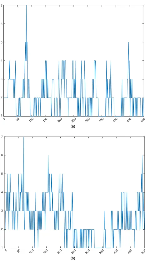
Figs 5(a)–5(d) and 6(a)–6(d) show the scatter plots and histograms of the simulated data and the predictive samples obtained by using the first calibration function, whereas Figs 5(e)– 5(h) and Figs 6(e)–6(h) show the scatter plots and histograms of the simulated data and the predictive sample obtained by using the second calibration function. The comparison between the simulated and predictive outputs highlights the excellent fit of the Bayesian non-parametric conditional copula model by using either calibration function and for different copula families. The model performance appears to be consistent across both copula families, demonstrating that the approach is suitable to model different dependence patterns and tail structures. Fig. 7 shows the plot of the number of components generated at each Markov chain Monte Carlo iteration for both the Gaussian and the Frank copula. In Fig. 7, we focus on the first calibration function, since the second calibration function gave similar results. Table 1 shows the summary statistics of the number of components that were generated at each Markov chain Monte Carlo iteration for both copulas, indicating that the posterior median of the number of components is equal to 2. For the two most significant components, we estimated the weights that were generated at each Markov chain Monte Carlo iteration for both copulas. In Fig. 8 we show the trace plots of the last 500 iterations of the first two weights, as defined in Section 4. Fig. 8 suggests that the first weight is much more important than the second weight, since the first weight tends to take values close to 1, whereas the second weight takes values close to 0. For each of the two components we also estimated the posterior mean of the copula correlation

(13)

0 0.1 0.2 0.3 0.4 0.5 0.6 0.7 0.8 0.9 1 0 0.1 0.2 0.3 0.4 0.5 0.6 0.7 0.8 0.9 1 0 0.1 0.2 0.3 0.4 0.5 0.6 0.7 0.8 0.9 1 0 0.1 0.2 0.3 0.4 0.5 0.6 0.7 0.8 0.9 1 0 0.1 0.2 0.3 0.4 0.5 0.6 0.7 0.8 0.9 1 0 0.1 0.2 0.3 0.4 0.5 0.6 0.7 0.8 0.9 1 0 0.1 0.2 0.3 0.4 0.5 0.6 0.7 0.8 0.9 1 0 0.1 0.2 0.3 0.4 0.5 0.6 0.7 0.8 0.9 1 (a) (b) (c) (d) (e) (f) (g) (h)

Fig. 5. Gaussian copula with sample sizenD500: (a), (c) scatter plots and (b), (d) histograms, obtained

with the first calibration function, of the simulated and predictive samples respectively; (e), (g) scatter plots and (f), (h) histograms, obtained with the second calibration function, of the simulated and predictive sample respectively

coefficientρj(defined in equation (5)), obtaining, for the Gaussian copula, a value of 0:6701 for

the first component and−0:9860 for the second component. In contrast, for the Frank copula

we obtained a posterior mean of 0:7941 for the first component and−0:9722 for the second

component.

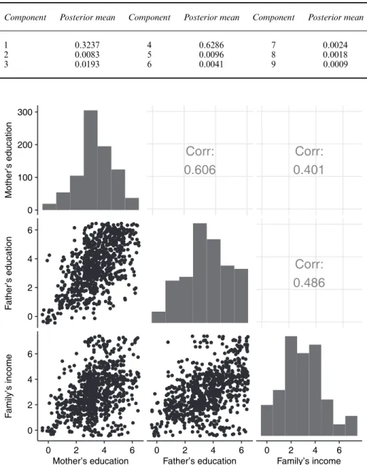
Finally, we consider an alternative Gaussian copula scenario, using the second calibration function. Table 2 shows the estimated weights of the mixture. The previous illustration, depicted in Fig. 8, showed that one component was dominating the others. In contrast, this experiment

shows two dominating weights,w1=0:3237 andw4=0:6286, motivating the use of the approach

proposed.

6. Real data application

We now apply the proposed Bayesian non-parametric conditional copula method to a sample of 839 adolescent twin pairs, which is a subset of the national merit twin study (Loehlin and

(14)

Copula Estimation of Twin Data 535 0 0.1 0.2 0.3 0.4 0.5 0.6 0.7 0.8 0.9 1 (a) (b) 0 0.1 0.2 0.3 0.4 0.5 0.6 0.7 0.8 0.9 1 (c) (d) 0 0.1 0.2 0.3 0.4 0.5 0.6 0.7 0.8 0.9 1 (e) _(f) 0 0.1 0.2 0.3 0.4 0.5 0.6 0.7 0.8 0.9 1 0 0.1 0.2 0.3 0.4 0.5 0.6 0.7 0.8 0.9 1 0 0.1 0.2 0.3 0.4 0.5 0.6 0.7 0.8 0.9 1 0 0.1 0.2 0.3 0.4 0.5 0.6 0.7 0.8 0.9 1 0 0.1 0.2 0.3 0.4 0.5 0.6 0.7 0.8 0.9 1 (g) (h)

Fig. 6. Frank copula with sample sizenD500: (a), (c) scatter plots and (b), (d) histograms, obtained with

the first calibration function, of the simulated and predictive samples respectively; (e), (g) scatter plots and (f), (h) histograms, obtained with the second calibration function, of the simulated and predictive sample respectively

Table 1. Summary statistics of the number of components generated at each Markov chain Monte Carlo iteration for the first calibration function

Copula Minimum 1st quantile Median Mean 3rd quantile Maximum

Gaussian 1 1 2 2.102 3 7

Frank 1 2 2 2.546 3 7

Nichols, 2009, 2014). The data set contains questionnaire data from 17-year-old twins and their parents, where the twins were identified among 600 000 US high school juniors who took part in the NMSQT.

The NMSQT was designed to measure cognitive aptitude, i.e. students’ readiness for future intellectual or educational pursuits. The participants in the test include identical twins and same-sex fraternal twins who were asked to fill in a complete questionnaire to understand their

(15)

1 2 3 4 5 6 7 (a) 0 ₅₀ 100 150 200 250 300 350 400 450 500 0 ₅₀ 100 150 200 250 300 350 400 450 500 1 2 3 4 5 6 7 (b)

Fig. 7. Number of components (y-axis) generated at each Markov chain Monte Carlo iteration (x-axis) for

(16)

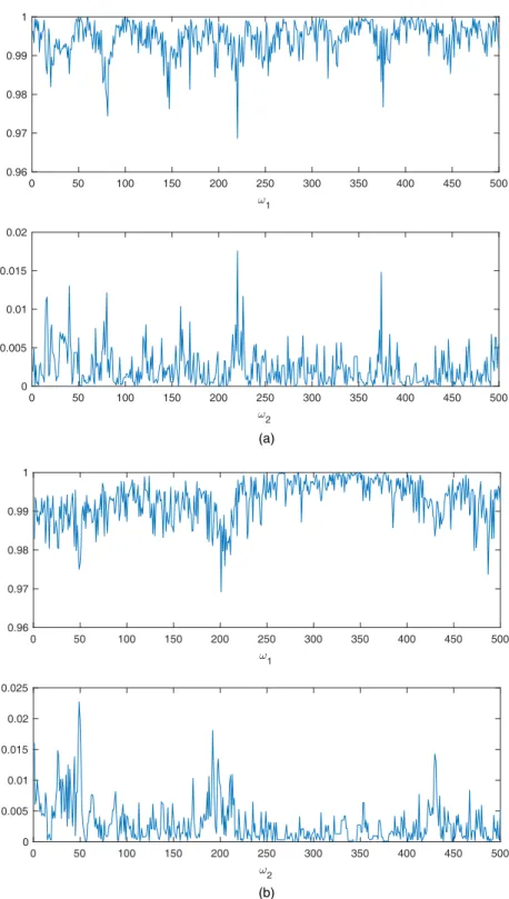
Copula Estimation of Twin Data 537 1 0.96 0.97 0.98 0.99 1 2 0 0.005 0.01 0.015 0.02 1 0.96 0.97 0.98 0.99 1 0 50 100 150 200 250 300 350 400 450 500 0 50 100 150 200 250 300 350 400 450 500 0 50 100 150 200 250 300 350 400 450 500 0 50 100 150 200 250 300 350 400 450 500 2 0 0.005 0.01 0.015 0.02 0.025 (a) (b)

Fig. 8. Plots of the values of the first two most significant weights (y-axis) generated at each Markov chain

Monte Carlo iteration (x-axis) for (a) the Gaussian and for (b) the Frank copula with sample sizenD500: the

values of the first weight are plotted in the top panels, whereas the values of the second weight are plotted in the bottom panels

(17)

Table 2. Posterior means of the weights obtained with the second calibration function and

sample sizenD500 for the Gaussian copula

Component Posterior mean Component Posterior mean Component Posterior mean

1 0.3237 4 0.6286 7 0.0024 2 0.0083 5 0.0096 8 0.0018 3 0.0193 6 0.0041 9 0.0009 Mother’s education F ather’s education F a mily’s income 0 100 200 300

Corr:

0.606 Corr:

0.401

0 2 4 6

Corr:

0.486

0 2 4 6 n F n F 0 2 4 6

Mother’s educatio ather’s educatio amily’s income

0 2 4 6 0 2 4 6

Fig. 9. Relationship between the covariates of the twins data set: the lower triangular panels represent pairwise scatter plots, the upper triangular panels show pairwise Pearson’s correlation coefficients and the diagonal panels represent the histograms of each covariate (note that jittering was used in the scatter plots to prevent overplotting)

school performance and attitude. Our purpose is to examine whether the relationship between twins’ cognitive ability, measured by the NMSQT, is influenced by their socio-economic status, measured by parent education and parental income. The variables that we considered from this study are the overall measures of each twin’s performance at school (obtained as the sum of individual scores in English usage, mathematics usage, social science reading, natural science

(18)

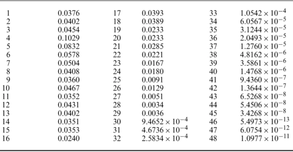
Table 3. Posterior means of the mixture component weights for the twins’ performance scores with respect to the mother’s level of education

Component Posterior mean Component Posterior mean Component Posterior mean

1 0.0376 17 0.0393 33 1:0542×10−4 2 0.0402 18 0.0389 34 6:0567×10−5 3 0.0454 19 0.0233 35 3:1244×10−5 4 0.1029 20 0.0233 36 2:0493×10−5 5 0.0832 21 0.0285 37 1:2760×10−5 6 0.0578 22 0.0221 38 4:8162×10−6 7 0.0504 23 0.0167 39 3:5861×10−6 8 0.0408 24 0.0180 40 1:4768×10−6 9 0.0360 25 0.0091 41 9:4360×10−7 10 0.0467 26 0.0129 42 1:3644×10−7 11 0.0352 27 0.0051 43 6:5268×10−8 12 0.0431 28 0.0034 44 5:4506×10−8 13 0.0402 29 0.0036 45 3:4268×10−8 14 0.0351 30 9:4652×10−4 46 5:4973×10−13 15 0.0353 31 4:6736×10−4 47 6:0754×10−12 16 0.0240 32 2:5834×10−4 48 1:0977×10−11

reading and word usage and vocabulary), the mother’s and father’s level of education and the family income. The overall scores range from 30 to 160, the education covariates range from 0 to 6 and the family income covariate ranges from 0 to 7. The levels of the education covariates correspond to less than eighth grade, eighth grade, part high school, high school graduate, part college or junior college, college graduate and graduate or professional degree beyond a Bachelor’s degree. The levels of the income covariate correspond to values going from less than $5000 per year to over $25 000 per year.

As discussed in Section 1, the scatter plots in Fig. 1 clearly show that there is a positive corre-lation between the twins’ school performance and the strength of dependence varies according to the values of a covariate, which is the mother’s (Fig. 1(a)) or father’s level of education (Fig. 1(b)) or the family income (Fig. 1(c)). In Fig. 1 the effect of the covariates is illustrated by dots of various shades, where we note that most of the light dots are grouped in the upper right-hand corner, whereas the dark dots lie in the bottom left-right-hand corner. Therefore, the higher the parents’ education or family income, the higher is the twins’ school performance. To model the effect of a covariate, such as the mother’s and father’s education and family income, on the dependence between the overall scores of the twins, we implement the Bayesian non-parametric conditional copula model.

Fig. 9 shows the relationship between the covariates of the twins data set, where the lower trian-gular panels represent pairwise scatterplots, the upper triantrian-gular panels show pairwise Pearson correlation coefficients and the diagonal panels represent the histograms of each covariate. The scatter plots and Pearson’s correlation coefficients in Fig. 9 indicate quite a strong positive corre-lation between each pair of covariates, especially between the mother’s and father’s level of edu-cation. The high correlations indicate that the data do not contain much information on the inde-pendent effects of each covariate and suggest the inclusion of only one of them in the model. For this reason we decided to include only one of the redundant covariates at a time. Note that, with a different data set, the methodology may be extended to include more than one covariate. How-ever, model specification issues and increased computational costs must be carefully considered. Adopting the same priors as those of the simulation studies, we run the Gibbs sampling algorithm described in Section 4 for 4000 iterations. Figs 10, 11 and 12 show, for the mother’s

(19)

L. Dalla V alle, F. Leisen and L. Rossini 20 40 60 80 100 120 140 160 180 (a) 0 0.1 0.2 0.3 0.4 0.5 0.6 0.7 0.8 0.9 1 (b) 20 40 60 80 100 120 140 160 180 (c) 20 40 60 80 100 120 140 160 0 0.1 0.2 0.3 0.4 0.5 0.6 0.7 0.8 0.9 1 20 40 60 80 100 120 140 160 180 0 0.1 0.2 0.3 0.4 0.5 0.6 0.7 0.8 0.9 1 0 0.1 0.2 0.3 0.4 0.5 0.6 0.7 0.8 0.9 1 (d) (e) (f)

Fig. 10. (a), (b) Scatter plots of the twins’ overall scores for the real and pseudo-observations with respect to the mother’s level of education; (c), (d) scatter plots of the predictive and transformed predictive samples; (e), (f) histograms of the real data and the predictive sample

(20)

Copula Estimation of T win Data 541 20 40 60 80 100 120 140 160 180 (a) 0 0.1 0.2 0.3 0.4 0.5 0.6 0.7 0.8 0.9 1 (b) 20 40 60 80 100 120 140 160 180 (c) 20 40 60 80 100 120 140 160 0 0.1 0.2 0.3 0.4 0.5 0.6 0.7 0.8 0.9 1 20 40 60 80 100 120 140 160 180 0 0.1 0.2 0.3 0.4 0.5 0.6 0.7 0.8 0.9 1 0 0.1 0.2 0.3 0.4 0.5 0.6 0.7 0.8 0.9 1 (d) (e) (f)

Fig. 11. (a), (b) Scatter plots of the twins’ overall scores for the real and pseudo-observations with respect to the father’s level of education; (c), (d) scatter plots of the predictive and transformed predictive samples; (e), (f) histograms of the real data and the predictive sample

(21)

L. Dalla V alle, F. Leisen and L. Rossini 20 40 60 80 100 120 140 160 180 (a) 0 0.1 0.2 0.3 0.4 0.5 0.6 0.7 0.8 0.9 1 (b) 20 40 60 80 100 120 140 160 180 (c) 20 40 60 80 100 120 140 160 0 0.1 0.2 0.3 0.4 0.5 0.6 0.7 0.8 0.9 1 20 40 60 80 100 120 140 160 0 0.1 0.2 0.3 0.4 0.5 0.6 0.7 0.8 0.9 1 0 0.1 0.2 0.3 0.4 0.5 0.6 0.7 0.8 0.9 1 (d) (e) (f)

Fig. 12. (a), (b) Scatter plots of the twins’ overall scores for the real and pseudo-observations with respect to family income; (c), (d) scatter plots of the

(22)

Table 4. Posterior means of the mixture component weights for the twins’ performance scores with respect to the father’s level of education

Component Posterior mean Component Posterior mean Component Posterior mean

1 0.0514 18 0.0313 35 7:4762×10−6 2 0.0516 19 0.0260 36 4:8028×10−6 3 0.0536 20 0.0257 37 3:5777×10−6 4 0.0379 21 0.0197 38 7:2414×10−7 5 0.0675 22 0.0246 39 5:6380×10−7 6 0.0743 23 0.0063 40 1:5620×10−7 7 0.0414 24 0.0097 41 5:4960×10−8 8 0.0523 25 0.0049 42 1:0994×10−7 9 0.0384 26 0.0037 43 1:5524×10−8 10 0.0497 27 0.0013 44 1:1536×10−8 11 0.0351 28 5:7852×10−4 ₄₅ ₆_:₄₅₁₆_×₁₀−9 12 0.0495 29 3:5660×10−4 46 6:2531×10−9 13 0.0304 30 1:6825×10−4 ₄₇ ₁_:₄₂₅₅_×₁₀−8 14 0.1066 31 9:9642×10−5 48 3:4571×10−9 15 0.0270 32 4:6900×10−5 ₄₉ ₇_:₀₁₂₃_×₁₀−10 16 0.0319 33 2:6103×10−5 50 1:8651×10−10 17 0.0469 34 1:1375×10−5 51 8:0720×10−10

Table 5. Posterior means of the mixture component weights for the twins’ performance scores with respect to the family income

Component Posterior mean Component Posterior mean Component Posterior mean

1 0.0836 17 0.0359 33 1:1455×10−4 2 0.0681 18 0.0236 34 6:7836×10−5 3 0.0486 19 0.0277 35 3:8637×10−5 4 0.0750 20 0.0233 36 1:9610×10−5 5 0.0074 21 0.0205 37 1:0765×10−5 6 0.0569 22 0.0209 38 6:4166×10−6 7 0.0492 23 0.0172 39 4:1155×10−6 8 0.0415 24 0.0105 40 2:7336×10−6 9 0.0319 25 0.0097 41 9:7839×10−7 10 0.0340 26 0.0080 42 3:6532×10−7 11 0.0288 27 0.0042 43 3:5966×10−7 12 0.0451 28 0.0023 44 1:7294×10−7 13 0.0395 29 0.0018 45 1:9279×10−8 14 0.0365 30 0.0013 46 1:5505×10−8 15 0.0281 31 4:1135×10−4 47 8:1074×10−9 16 0.0377 32 2:2382×10−4 ₄₈ ₈_:₅₉₉₆_×₁₀−9

and father’s education and family income respectively, the scatter plots of the twins’ overall scores by using the real and transformed pseudo-observations (Figs 10(a), 10(b), 11(a), 11(b), 12(a) and 12(b)), the scatter plots of the predictive and transformed predictive samples (Figs 10(c), 10(d), 11(c), 11(d), 12(c) and 12(d)) and the histograms of the real and the predictive samples (Figs 10(e), 10(f), 11(e), 11(f), 12(e) and 12(f)). Note that the pseudo-observations are obtained by using the non-parametric estimation approach that was described in Section 4. From the comparison between the scatter plots and histograms of the real and predictive samples obtained with the three different covariates, it emerges that the Bayesian non-parametrics conditional

(23)

Mother‘s level of education 0.2 0.3 0.4 0.5 0.6 0.7 0.8 0.9

Conditional Kendall‘s tau

(a)

Father‘s level of education

0.2 0.3 0.4 0.5 0.6 0.7 0.8 0.9

(b) 0 1 2 3 4 5 6 0 1 2 3 4 5 6 0 1 2 3 4 5 6 7 Family Income 0.2 0.3 0.4 0.5 0.6 0.7 0.8 0.9

(c)

Fig. 13. Estimated Kendall’sτagainst (a) the mother’s and (b) the father’s level of education and (c) family

(24)

copula model accurately captures the tail structures and the dependence patterns between the twins’ overall scores. Moreover, the posterior means of the number of mixture components

for the conditional copula are 26:82, 24:49 and 27:11, for the mother’s and father’s level of

education and the family income respectively, supporting the need for non-Gaussian copulas. Tables 3, 4 and 5 list the posterior means of the component weights when the three covariates are considered. We note that the good performance of this approach in tail modelling makes it suitable for various applications focusing on extremes. To quantify the degree of dependence

between the twins’ scores, we use the conditional Kendall’sτ, which is a non-parametric measure

of correlation, known as concordance, between two ranked variables.Y1,Y2/with respect to a

covariateX=x. The conditional Kendall’sτtakes the form

τ.x/=4 Cx.u1,u2/dCx.u1,u2/−1

whereCxis the appropriate conditional copula. Fig. 13 shows Kendall’sτ estimated from the

model against the mother’s (Fig. 13(a)) and father’s level of education (Fig. 13(b)) and the family income (Fig. 13(c)), together with 95% credible intervals. The plots clearly illustrate the negative effect of all three covariates on the dependence between the twins’ overall scores. The effect is

greater for family income, where Kendall’sτdecreases from approximately 0:83 to 0:45, whereas

for the parents’ education levels Kendall’sτdecreases from approximately 0:8 to 0:6. Therefore,

the higher the parents’ education and family income, the better the socio-economic status is and the higher the differences between the twins’ school performances. The cognitive aptitudes of twins from less advantaged families are more similar to each other than those from high income, highly educated families. Families of high socio-economic status provide supportive and challenging environments, which can offer a wide range of opportunities and choices to their children, and allow them to express themselves freely. Hence, twins raised in wealthy families are encouraged to develop differences in their traits and may show quite dissimilar cognitive abilities, albeit high on average. In contrast, families of low socio-economic status offer scarce opportunities to their children and may provide limiting and restrictive environments. In less advantaged families, twins cannot develop their full potential and individuality; hence both tend to show low cognitive abilities.

This might suggest, as in Loehlinet al.(2009), an interaction between genetic and

environmen-tal factors. Genes multiply environmenenvironmen-tal inputs that support intellectual growth such that an increased socio-economic status raises the average cognitive ability but also magnifies individual

differences in cognitive ability (see Bateset al.(2013)).

7. Conclusion

In this paper we proposed a Bayesian non-parametric conditional copula approach to model the strength and type of dependence between two variables of interest and we applied the methodology to the national merit twin study. To capture the dependence structure between two variables, we introduced two different calibration functions expressing the functional form of a covariate variable. The statistical inference was obtained by implementing a slice sampling algorithm, assuming an infinite mixture model for the copula. The methodology combines the advantages of the conditional copula approach with the modelling flexibility of Bayesian non-parametrics.

The simulation studies illustrated the excellent performance of our model with three distinct copula families and different sample sizes. The application to the twins data revealed the

(25)

im-portance of the environment in the development of twins’ cognitive abilities and suggests that environmental factors are more influential in families with higher socio-economic position. In contrast, other factors, such as genetic causes, may be more dominant in families with lower socio-economic position.

Although this paper focuses on bivariate copula models, the methodology can be extended to multivariate copulas including more than one covariate. However, the inclusion of multiple covariates needs special attention regarding the choice of variables before estimating the cali-bration functions. Moreover, the increasing computational cost due to the additional covariates should be taken carefully into consideration.

Acknowledgements

The authors are grateful to the Associate Editor and the reviewers for their useful comments which significantly improved the quality of the paper. Fabrizio Leisen was supported by the Eu-ropean Community’s seventh framework programme (FP7/2007-2013) under grant agreement 630677.

Appendix A: Gibbs sampling details

LetDj={i=1,: : :,n:di=j}be the set of indices of the observations allocated to thejth component of the mixture, whereasD={j:Dj= ∅}is the set of indices of non-empty mixtures components. Let

DÅ=sup{D}be the number of stick breaking components that are used in the mixture. As in Kalliet al. (2011), the sampling of infinite elements ofπandβis not necessary, since only the elements of the full conditional probability density functions ofDare needed.

The maximum number of stick breaking components to be sampled is

NÅ=max{i=1,: : :,n|NÅ_i}, whereNÅ_i is the smallest integer such thatΣNÆi

j=1wj>1−zi. A.1. Update ofπ

We update the stick breaking components and consequently the weightswjbased on the equation

wj=πj

k<j

.1−πk/:

Assuming thatπjis distributed as a beta (Be.1,λ/) distribution, the full conditional distribution ofπjis

πj|: : :∼Be.1+#{di=j},λ+#{di> j}/, .14/ where #{di=j}is the number ofdiequal tojand #{di> j}is the number ofdigreater thanjforj < DÅ.

In contrast, ifj=DÅ+1,: : :,NÅwe have that

πj|: : :∼Be.1,λ/:

A.2. Update ofZ

From the full likelihood function (13),zifollows a uniform distribution

zi|: : :∼U.0,wdi/ .15/

(26)

A.3. Update ofD

The allocation variabledivalues lie between 0 andNiand the density ofdisatisfies

P.di=j|: : :/∝I.zi<wdi/cρ.xi|βdi/.ui,vi/: .16/ A.4. Update ofβ

The full conditional of the vector of parametersβk, fork1, is

f.β_k|: : :/∝π.β_k/

di=k

cρ.xi|βk/.ui,vi/, .17/ whereπ.β_k/is the prior onβ. Since expression (17) is not a standard distribution, we used a random-walk Metropolis–Hastings algorithm.

References

Abegaz, F., Gijbels, I. and Veraverbeke, N. (2012) Semiparametric estimation of conditional copulas.J. Multiv. Anal.,110_{, 43–73.}

Acar, E. F., Craiu, R. V. and Yao, F. (2010) Dependence calibration in conditional copulas: a nonparametric approach.Biometrics,67, 445–453.

Andersen, E. (2005) Two-stage estimation in copula models used in family studies.Liftim. Data Anal.,11_{, 333–} 350.

Baker, S. (2016) The latent class twin method.Biometrics,3_{, 827–834.}

Bartram, S., Taylor, S. and Wang, Y. (2007) The Euro and European financial market dependence.J. Bankng Finan.,31, 1461–1481.

Bates, T., Lewis, G. and Weiss, A. (2013) Childhood socioeconomic status amplifies genetic effects on adult intelligence.Psychol. Sci.,24, 2111–2116.

Braekers, R. and Veraverbeke, N. (2005) A copula-graphic estimator for the conditional survival function under dependent censoring.Can. J. Statist.,33_{, 429–447.}

Burda, M. and Prokhorov, A. (2014) Copula based factorization in Bayesian multivariate infinite mixture models. J. Multiv. Anal.,127_{, 200–213.}

Cherubini, U., Luciano, E. and Vecchiato, W. (2004)Copula Methods in Finance. Chichester: Wiley.

Craiu, R. V. and Sabeti, A. (2012) In mixed company: Bayesian inference for bivariate conditional copula models with discrete and continuous outcomes.J. Multiv. Anal.,110_{, 106–120.}

Emura, T. and Wang, W. (2012) Nonparametric maximum likelihood estimation for dependent truncation data based on copulas.J. Multiv. Anal.,110, 171–188.

Escobar, M. D. (1994) Estimating normal means with a Dirichlet process prior.J. Am. Statist. Ass.,89_{, 268–} 277.

Escobar, M. D. and West, M. (1995) Bayesian density estimation and inference using mixtures.J. Am. Statist. Ass.,90_{, 577–588.}

Ferguson, T. (1983)Bayesian Density Estimation by Mixtures of Normal Distributions, pp. 287–303. New York: Academic Press.

Gijbels, I., Omelka, M. and Veraverbeke, N. (2012) Multivariate and functional covariates and conditional copulas. Electron. J. Statist.,6, 1273–1306.

Gijbels, I., Veraverbeke, N. and Omelka, M. (2011) Conditional copulas, association measures and their applica-tions.Computnl Statist. Data Anal.,55, 1919–1932.

Huang, X. and Zhang, N. (2008) Regression survival analysis with an assumed copula for dependent censoring: a sensitivity analysis approach.Biometrics,64_{, 1090–1099.}

Joe, H. (2014)Dependence Modeling with Copulas. Boca Raton: Chapman and Hall.

Jondeau, E. and Rockinger, M. (2006) The copula-GARCH model of conditional dependencies: an international stock market application.J. Int. Mon. Finan.,25_{, 827–853.}

Kalli, M., Griffin, J. E. and Walker, S. G. (2011) Slice sampling mixture models.Statist. Comput.,21, 93–105. Klein, N. and Kneiss, T. (2016) Simultaneous inference in structured additive conditional copula regression

models: a unifying Bayesian approach.Statist. Comput.,26_{, 841–860.}

Kolev, N., dos Anjos, U. and Vaz de Mendes, B. (2006) Copulas: a review and recent developments.Stochast. Modls,22_{, 617–660.}

Lo, A. (1984) On a class of Bayesian nonparametric estimates: I, density estimates.Ann. Statist.,12_{, 351–357.} Loehlin, J., Harden, K. and Turkheimer, E. (2009) The effect of assumptions about parental assortative mating

and genotype–income correlation on estimates of genotype–environment interaction in the national merit twin study.Behav. Genet.,39, 165–169.

Loehlin, J. and Nichols, R. (2009) The National Merit twin study. InHarvard Dataverse, vol. 3. (Available from http://hdl.handle.net/1902.1/13913.)

(27)

Loehlin, J. and Nichols, R. (2014)Heredity, Environment and Personality: a Study of 850 Sets of Twins. Austin: University of Texas Press.

Owzar, K., Jung, S.-H. and Sen, P. K. (2007) A copula approach for detecting prognostic genes associated with survival outcome in microarray studies.Biometrics,63_{, 1089–1098.}

Patton, A. J. (2006) Modelling asymmetric exchange rate dependence.Int. Econ. Rev.,47_{, 527–556.}

Pitt, M., Chan, D. and Kohn, R. (2006) Efficient Bayesian inference for Gaussian copula regression models. Biometrika.,93_{, 537–554.}

Plummer, M. (2008) Penalized loss functions for bayesian model comparison.Biostatistics,9_{, 523–539.} Sklar, A. (1959) Fonctions de r´eparation `a n dimensions et leurs marges.Publ. Inst. Statist. Univ. Paris,8, 229–

231.

Smith, M. S., Gan, Q. and Kohn, R. J. (2012) Modelling dependence using skewtcopulas: Bayesian inference and applications.J. Appl. Econmetr.,27, 500–522.

Stander, J., Dalla Valle, L., Taglioni, C. and Cortina Borja, M. (2015a) Bayesian copula modelling in the presence of covariates. InBook of Abstracts, 8th Int. Conf. European Consortium for Informatics and Working Group on Computational and Methodological Statistics(eds A. Blanco-Fernandez and G. Gonzalez-Rodriguez), p. 179. London: CFE and Computational and Methodological Statistics.

Stander, J., Dalla Valle, L., Taglioni, C. and Cortina Borja, M. (2015b) Bayesian copula modelling in the presence of covariates.Royal Statistical Society Conf., Exeter.

Taglioni, C., Stander, J., Dalla Valle, L. and Cortina-Borja, M. (2016) Bayesian copula modelling in the presence of covariates. InBook of Abstracts, Wrld Meet. Bayesian Statistics, Cagliari(eds S. Cabras and M. Guindani), pp. 413–414. Cagliari: Cooperativa Universitaria Editrice Cagliaritana.

Walker, S. G. (2007) Sampling the Dirichlet mixture model with slices.Communs Statist. Simuln Computn,36_, 45–54.

Wang, X., Guo, X., He, M. and Zhang, H. (2011) Statistical inference in mixed models and analysis of twin and family data.Biometrics,67_{, 987–995.}

Wu, J., Wang, X. and Walker, S. (2015) Bayesian nonparametric estimation of a copula.J. Statist. Computn Simuln,85_{, 103–116.}

Yin, G. and Yuan, Y. (2009) Bayesian dose finding in oncology for drug combinations by copula regression.Appl. Statist.,58_{, 211–224.}