Hitotsubashi University Repository
Author(s) Gørgens, Tue; Meng, Xin; Vaithianathan, Rhema
Citation
Issue Date 2010-10
Type Technical Report
Text Version publisher
URL http://hdl.handle.net/10086/18732
PRIMCED Discussion Paper Series, No. 2
Stunting and Selection Effects of Famine:
A Case Study of the Great Chinese Famine
Tue Gørgens, Xin Meng, and Rhema Vaithianathan
October 2010
Research Project PRIMCED Institute of Economic Research
Hitotsubashi University 2-1 Naka, Kunitatchi Tokyo, 186-8601 Japan http://www.ier.hit-u.ac.jp/primced/e-index.html
A Case Study of the Great Chinese Famine
∗
Tue Gørgens
†Xin Meng
‡Rhema Vaithianathan
§October 2010
Abstract: Many developing countries experience famine. If survival is related to height, the increasingly common practice of using height as a measure of well-being may be misleading. We devise a novel method for disentangling the stunting from the selection effects of famine. Using data from the 1959–1961 Great Chinese Famine, we find that taller children were more likely to survive the famine. Controlling for selection, we estimate that children under the age of five who survived the famine grew up to be 1 to 2 cm shorter. Our results suggest that average height is potentially a biased measure of economic conditions during childhood.
Keywords: Famine, height, China, panel data. JEL classification numbers: C33, I12, N950, O15.
∗We thank colleagues and visitors at the Australian National University, too numerous to mention by
name, for comments on earlier drafts of this paper.
†Social Policy Evaluation, Analysis and Research (SPEAR) Centre, Research School of Economics,
Australian National University, Canberra 0200, Australia. E-mail: Tue.Gorgens@anu.edu.au.
‡Research School of Economics, Australian National University, Canberra 0200, Australia. E-mail:
Xin.Meng@anu.edu.au.
§Department of Economics, University of Auckland, Private Bag 92019, Auckland 1020, New Zealand.
1
Introduction
Height is closely related to nutritional intake during childhood. Height is therefore in-creasingly used as an indirect measure of the material conditions that prevailed during childhood in developing country and historical settings, where direct measures of economic conditions are unavailable or unreliable (e.g. Fogel et al., 1982; Fogel, 1994; Steckel, 1995; Micklewright and Ismail, 2001). For example, Deaton (2008) utilizes inequality of height to draw inferences about overall economic inequality in India. Height has also been utilized to measure access to resources in early childhood (e.g. Alderman, Hoddinott, and Kinsey, 2006), intra-family resource allocation (e.g. Duflo, 2003), and the effect of income growth on nutrition (e.g. O’Donnell, Nicolas, and Doorslaer, 2008). When childhood mortality rates are high and if taller children are more likely to survive, bias due to height-related selection can be an added complications for these studies.
The concern that survivor-bias may confound the correlation between height and eco-nomic welfare is not new (e.g. Vaupel et al., 1979; Waaler, 1984). Friedman (1982) notes it as a possible explanation for the increased height of slaves in Trinidad. More recently, Boz-zoli, Deaton, and Quintana-Domeque (2007) find that population height increases with the mortality rate for countries whose infant mortality rate exceeds a threshold level. They argue that this might be associated with selection effects and could contribute to explaining the extraordinary height of Africans.
The Great Chinese Famine of 1959–1961 provides a useful case study for exploring the selection effects of high childhood mortality. People exposed to famine during childhood may be stunted in the sense that they become shorter adults than they would otherwise have been. However, famine may also cause height-related selection of survivors. If children who in the absence of famine would grow up to be relatively short are less likely to survive a famine, then the survivors may be taller everything else being equal (e.g. Smedman et al., 1987; Razzaque et al., 1990; Bairagi and Chowdhury, 1994; Fawzi et al., 1997; Yan, 1999; Schultz, 2001). If selection outweighs stunting, famines create taller populations, which may be mistakenly interpreted as evidence of an improvement in economic conditions.
This paper considers the long-term effect of the Great Chinese Famine on the height of the survivors. China’s Great Famine was one of the worst human catastrophes of the 20th Century. It is estimated that the famine caused 30 million excess deaths (e.g. Lin and Yang, 1998). Yet it is only recently that researchers have started to piece together its long-term consequences (see e.g. ´O Gr´ada, 2008, for a recent survey). Schultz (2001, p26) points out the importance of disentangling the stunting and selection effects of the Chinese famine but argues that “there is insufficient time-series evidence on mortality and health series indicators to know under what conditions one empirical force (i.e. stunting or selection by mortality) would dominate”.
The main objective of this paper is to estimate the stunting and selection effects of the famine. As far as we are aware, this is the first such attempt in the literature. To disentangle the stunting and selection effects, we devise a novel and powerful econometric strategy. The basic idea is simple. Children inherit their parents’ genotype (selection) and not their phenotype (stunting). If famine survivors have greater average potential height due to selection, then their children will inherit this potential and be taller than children of the control group. Conversely, if survivors have shorter potential height, their children will be shorter than the control group. Therefore, we can use children of cohorts who were exposed to famine during early childhood and children of cohorts who were less affected by famine to control for selection.
Controlling for selection, we find that rural people who were exposed to the famine in the first 5 years of life are stunted between 1 and 2 cm. The econometric model also allows us to estimate the selection effects. We estimate that height-related selection has increased the average height of rural female famine survivors by about 2 cm and the average height of rural male survivors by about 1 cm, although the latter is not statistically significant. Selection effects of 1 to 2 cm are economically significant. To put these estimates in perspective, the average height of 20–25 year-old Chinese increased by 2.8 cm between 1997 and 2006, a period when the Chinese per capita real GDP increased by more than 150%. Moreover, our results have broad relevance in the developing world. Although China’s Great Famine is unprecedented in terms of sheer scale, we argue in Section 7 that
the actual child mortality rates may be comparable with other famines such as the 1974– 1975 Bangladesh famine (e.g. Chen, Rahman, and Sarder, 1980) and the 2000 Ethiopian famine (e.g. Salama, Assefa, Talley, Spiegel, van der Veen, and Gotway, 2001). One would expect similar selection effects during those famines.
Our results are also relevant beyond famine settings. Whenever height is compared across populations where there are large differences in child mortality rates, selection is a potential issue. Infant mortality rates differ by more than a factor of three across Indian states (e.g. Bhalotra, 2007) and by more than a factor of ten across OECD countries (e.g. Bozzoli, Deaton, and Quintana-Domeque, 2007). Our findings therefore sounds a caution that height may potentially be a biased measure of economic conditions across environments with large variance in infant mortality.
This paper is set out as follows. Section 2 provides an overview of the Chinese famine. Section 3 discusses the genetic and environmental factors which determine the height of a person and the relationship between the height of parents and children. Section 4 describes the data. In Section 5, we conduct some preliminary analysis, while Section 6 presents the econometric model and our estimation strategies. The results are discussed in Section 7. In Section 8 we examine the robustness of our results. Section 9 concludes the paper.
2
The Great Chinese Famine
The Great Chinese Famine started in 1959 and ended in 1961. There is still some con-troversy over the exact cause of the famine, although it was certainly associated with a reduction in grain output resulting from disruption in production attending the Great Leap Forward campaign and the collectivization of agriculture (e.g. Yao, 1999). This caused a drastic fall in grain production in 1959. However, it is generally accepted that the decline in food availability alone did not cause the estimated 20 to 30 million excess deaths between 1958 and 1961.
It is widely held that overzealous officials, keen to make a good impression about the success of collectivization, exaggerated grain production. The central planners therefore,
mistakenly believing there to be adequate grain supplies, exported rice, continued the wasteful practice of providing free meals in communal dining halls (e.g. Yang and Su, 1998) and acquired large amounts of grain for urban populations (e.g. Johnson, 1998; Lin and Yang, 2000). Widespread famine in the rural areas quickly followed.
Why the famine ended is still not certain. Johnson (1998) argues that it was associ-ated with a wide array of policy changes including the abolition of communal kitchens, importation of grain, and a reduction in the urban appropriation of grain. Land was returned to peasant control and collectivization scaled back (e.g. Yang and Su, 1998).
Because of the lack of contemporaneous evidence, researchers have relied on mortality figures from the China statistical yearbook of 1983 to piece together what happened during this crisis (e.g. Coale and Banister, 1994; Lin and Yang, 2000; Wei and Yang, 2005). Riskin (1998) however points out that the reliability of the mortality statistics published in the Chinese Yearbook for the famine period cannot be corroborated since there is little information about how mortality was calculated.
Although the famine lasted only a short time, between 1957 and 1960 the national average death rates increased from 10.8 to 25.4 per 1,000 and the birth rate during the same period fell from 34 to 21 per 1,000 (e.g. Lin and Yang, 1998). From the perspective of excess deaths, the Great Chinese Famine outstrips any other recorded famine (e.g. Smil, 1999).1
During the 1950s, China was mainly a rural society, with 85% of the total population classified as rural dwellers. As Lin and Yang (2000) point out, even though farmers produced grain products, the centralized distribution and the urban-biased development strategy implied that when food was limited the rural population had to sacrifice their consumption. While both urban and rural populations experienced an increase in their mortality rate during the famine years, the urban death rate in 1960 was 1.6 times the pre-famine rate, while the rural rate over the same time period rose by a factor of 2.6.
There is also evidence that females suffered more than males. Coale and Banister (1994) use data from four censuses that were held between 1953 to 1990 as well as
retro-1However, the actual death rates during the Irish famine of 1845–1849 and the Bengali famine of 1943
spective fertility surveys conducted in 1982 and 1988 to study the cohort-specific mortality rates. They find that although the gap between male and female mortality rates declined over the course of the 20th century, the decline was interrupted for cohorts who were children during the time of the famine. For these cohorts, girls were around 7% more likely to die than boys. They attribute this to a general neglect of female health and food intake during the famine, reflecting a cultural bias towards boys. They suggest that girls bore the brunt of the excess deaths caused by the famine.
There are to date a few papers that have found long-term consequences of the Chinese famine. St Clair et al. (2005) find that famine cohorts have an elevated risk of schizophre-nia. Yan (1999) looks for long-term stunting by plotting the average height of females and males. She finds a reduction in average height for males born in the famine years, whereas for females she observes a peculiar spike in height. Chen and Zhou (2007) in-vestigate how the height of survivors vary across birth years and provincial death rates. They report that people who were young during the famine are shorter than people born afterwards, and that the difference is larger the higher the (excess) death rate. They did not attempt to control for selection. Almond, Edlund, Li, and Zhang (2007) analyze the effect of exposure in utero to the Chinese famine. Utilizing Census data, they find that the famine group fared less well on a range of socio-economic factors than the control groups.
3
Determination of Height
The objective of this paper is to estimate the stunting and selection effects of famine. Our estimating strategy relies on comparing the cohorts who experienced famine at a young age with a control group of people who were either older during the famine or born after the famine.
To define the famine cohorts, one needs to understand the effect of famine on differ-ent age groups and to select those age groups which were most severely affected. While we have no information on the age profile of those who died during the Chinese famine, Salama et al. (2001) follow a sample of Ethiopians through a short famine period
(Decem-ber 1999 to July 2000) and find that 54% of those who died were children less than 5 years of age and 25% were children between 5 and 14. Other evidence confirms that nutritional deficiencies in early childhood are more important for determining adult height than de-ficiencies later in childhood (e.g. Micklewright and Ismail, 2001; Glewwe and King, 2000; Hoddinott and Kinsey, 2001). To allow for this, we define two famine cohorts. The “old famine cohort” consists of those born between 1948 and 1956; they were aged between 5 and 13 in 1961. The “young famine cohort” consists of those born between 1957 and 1961, who were aged under 5 during the famine.
The control group is defined as those who were born up to 10 years immediately before (1938 to 1947) and immediately after (1962 to 1971) the famine cohorts. The control group is chosen so as to extract a reasonably sized sample, while at the same time ensuring that it is close to the famine cohorts in birth years in order to minimize the possible impact of economic growth on height. In the following, we refer to the “pre-famine control group” and the “post-famine control group” which together make up “the control group”.
To disentangle stunting from selection, we make use of the height of children of the famine cohorts and the control group. It is convenient to denote the famine cohorts and the control group the “parents” and their offspring the “children”, although it should be kept in mind that many of the “parents” were children during the famine years and that some of the “children” are young adults (and even parents) at the time of data collection. It is not feasible to control for selection in a standard difference-in-differences estima-tion method. In particular, the children of the famine cohorts and the control group are not of the same age at the time their height is measured, and economic progress means that those born more recently have greater height potential than those born earlier. Other factors, such as differences in family size and mothers’ age when giving birth, may also contribute to a difference in average height between children. To take these factors into account in the estimation, we develop an econometric model of the relationship between the heights of parents and their children.
Let subscript i indicate a particular family. Each family consists of a mother, a father, and one or more children. Accordingly, we index the family members by j =
m, f,1, . . . , J.2 Let subscript t indicate the time of measurement.
A person’s height at time t is determined by three major influences (e.g. Schultz, 2002): genetic factors including hormonal and biochemical factors, environmental factors which influence nutrition and health conditions during childhood, and his/her age at the time of measurement. Let hijt denote the height of the jth individual in the ith family in period t. Then
hijt=f(ageijt,sexij) +Gij +Eij+Uijt, j =m, f,1, . . . , J, (1)
where f is some function of age and sex, Gij represents the effect of genetic factors, Eij the effect of environmental factors, and Uijt is measurement error. Note that we assume
Eij does not vary across time. The heights of the family members are related through both genetic factors and common environmental factors.
Medical research suggests that up to 60% of the height variation in a population can be attributed to genetic factors, but the exact inheritance process is not well understood (e.g. Ginsburg et al., 1998). A simple model of heritability (e.g. Goldberger, 1978) postulates that
Gij =τmGim+τfGif + ˜Gij, j = 1, . . . , J, (2)
where Gim and Gif are the genotypes of the mother and father, τm and τf are weights with τm +τf = 1, and ˜Gij is an individual-specific component. The latter is assumed to have mean 0 and be uncorrelated with Gim and Gif. There is no evidence that genes on the X or the Y chromosomes have any major effects (e.g. Carter and Marshall, 1978), whence it may be assumed that τm and τf both equal 1/2.3
The influence of environmental factors is not well understood either (e.g. Tanner, 1981). Environmental factors such as restrictions on diet, exposure to diseases and phys-ical activity can retard height. These environmental factors are affected by family and community characteristics. Parental income and education (e.g. Hoddinott and Kinsey, 2001) and birth order (e.g. Horton, 1986) have all been found to be relevant in explaining
2For simplicity, the notationJ does not explicitly differentiate between families of different size. 3We test the sensitivity of our results to this assumption in Section 7.
stature. The supply of public health services and clean drinking water are also important as chronic diarrhoea is a major cause of stunting in poor communities (e.g. Moore et al., 2001). In this paper, we focus on famine as a key environmental factor that determines height.
A model of the effect of environmental factors on height must accommodate unob-served as well as obunob-served factors. It is particularly important to allow for unobunob-served factors which are common to all members of a family, because the characteristics of the local environment, socioeconomic status and lifestyle are strongly correlated between gen-erations, which means that parents’ nutritional intake, health and treatment in case of illness when young may be similar to that of their children.
An error-components model is highly flexible and well suited for our purposes. Sin-gling out exposure to famine as an important determinant, we decompose the effect of environmental factors on parents’ and children’s height as follows:
Eij =Fij αj +Eijo +Eic+ ˜Eij, j =m, f, (3)
Eij =Eijo +Eic+ ˜Eij, j = 1, . . . , J, (4)
whereFij = (Fijo, Fijy) is a vector whose two components indicate if the individual belongs the old famine cohort (Fijo = 1, Fijy = 0), the young famine cohort (Fijo = 0, Fijy = 1), or the control group (Fijo = 0, Fijy = 0), the parameter αj = (αoj, αyj) is the amount of famine-related stunting for the old and the young famine cohorts, Eijo represents the effect of other observed factors (see Section 5), Eic represents the effect of unobserved factors which are common to all members of family i, and ˜Eij the effect of unobserved factors which are specific to individual j. The latter is assumed to be uncorrelated with the observed and the unobserved common factors.
There are no famine dummies in the children’s equations (Equation (4)), because no one in the second generation grew up during the Great Famine. Moreover, we exclude the parents’ famine dummies from the children’s equations, on the assumption that whether or not a parent experienced famine during his/her own childhood has no direct effect on their children’s height. Indirect effects through Eijo and Eic are allowed. For example,
the assumption does not rule out that on average parents in the famine cohorts feed their children better than parents in the control group. However, the difference must have arisen because parents who feed their children better were more likely to survive the famine (a selection effect throughEic), not because the famine caused survivors to change feeding patterns. Similarly, the assumption precludes inheritable changes in the genetic expression of stature as a result of famine (i.e. epigenetic effects on height).4 Finally, we exclude each parent’s famine dummy from the spouse’s equation, because the fact that a person suffered famine during childhood cannot directly affect the partner’s adult height. The assumptions that Fim and Fif do not appear in the spouse’s nor in the children’s equations are crucial for identifying the stunting effects.
Combining equations (1), (2) and (3) yields the following model. The heights of each member of family i in time period t are given by
himt =f(ageimt,sexim) +Fim αm+Eimo +Gim+Eic + ˜Eim+Uimt,
hift =f(ageift,sexif) +Fif αf +Eifo +Gif +Eic+ ˜Eif +Uift,
hi1t=f(agei1t,sexi1) +Eio1+τmGim+τfGif +Eic+ ˜Gi1+ ˜Ei1+Ui1t, ..
.
hiJt=f(ageiJt,sexiJ) +EiJo +τmGim+τfGif +Eic+ ˜GiJ + ˜EiJ +UiJt,
(5)
where the unobserved specific variables ˜Gij, ˜Eij and Uijt are assumed to be uncorrelated with the observed variables as well as with the unobserved common variables, Gim, Gif and Eic.
Model (5) is designed to estimate the stunting effects of the famine, as captured by the parameters αm and αf, while allowing for the possibility of selection. The model is consistent with a wide range of selection mechanisms. There are several possible reasons why famine survivors may have different potential height from non-survivors, and we now
4In other words, our estimation strategy assumes that exposure to famine has no effect on the genes of
the children of famine victims except through selection. There is some evidence that mothers who were in utero during the Dutch famine have lower birth-weight babies (e.g. Lumey, 1992), that poor nutrition of grandparents can change the inherited susceptibility to cardiovascular disease and diabetes (e.g. Kaati, Bygren, and Edvinsson, 2002), and that exposure to famine in utero of women increases their propensity to have daughters (e.g. Almond, Edlund, Li, and Zhang, 2007). We have found no evidence that nutrition affects the expression of genes associated with stature, although this remains a possibility.
turn to a discussion of these.
In principle, the selection effect on the potential height of survivors may be either positive or negative. Deaton (2005) speculates that shorter people may be more efficient at using food than taller people and therefore more able to survive. If this hypothesis is true, then we would expect any selection effects to exacerbate the stunting effects, and for the children of famine survivors to be shorter.
On the other hand, there is some evidence of positive selection in the literature. Fawzi et al. (1997) study Sudanese children between 6 months and 6 years of age during a famine and find that after adjusting for a number of factors including age, sex, socio-economic status, and vitamin A levels, children in the shortest height-for-age category have a sig-nificantly higher mortality rate than taller children. Smedman et al. (1987) find similar results for children in Guinea-Bassau. There is also evidence of a negative relationship between mortality and height more generally. Using a large sample of Norwegian indi-viduals, Waaler (1984) found a clear reduction in mortality with increased body height. Waaler’s findings have been corroborated on Swedish data by Peck and Vagero (1989) and British data by Leon et al. (1995). Kemkes-Grottenthaler (2005) investigated age of death and height of skeletons from various time periods. She found that taller individuals had a considerably longer life-expectancy.
Selection may result not only from excess mortality, but also from lowered fertility. Birth rates fell dramatically during the famine (e.g. Coale and Banister, 1994). The famine cohorts born between 1959 and 1961 are therefore censored. From the point of view of estimating the stunting of famine survivors, people who were never born do not pose a separate problem from people who were born but did not survive.
Our model accommodates all of these potential selection effects by allowing Gim,Gif and Eic to be correlated with Fim and Fif. That is, famine survivors may have larger or smaller values of Gim, Gif and Eic than the control group who did not experience famine during their childhood.5 These differential values will be passed on to their children, who as a consequence will be taller or shorter than children whose parents are in the control
5Survival probabilities may also be related to factors unrelated to height, but that is not a concern
group.
In closing this section, we note that the biological literature has identified assortative mating as a major confounding factor in the analysis of the inheritability of height (e.g. Carter and Marshall, 1978; Ginsburg et al., 1998). It is well established that people tend to marry people of similar characteristics, be it education, socio-economic status, or height. Thus, while there can be no direct effect of the father’s stunting and selection effects on the mother’s height and vice versa, there may be an indirect effect because of assortative mating: a man who is stunted is more likely to marry a short woman, and therefore more likely to marry a woman who is short for genetic reasons. Our model accommodates assortative mating behavior by allowing the mother’s and the father’s observed and unobserved variables to be correlated.
4
Data, Famine Cohorts and Control Group
The data used in this study are from the China Health and Nutrition Survey (CHNS) con-ducted by the Carolina Population Center at University of North Carolina at Chapel Hill. We use the first four waves of the panel. The CHNS contains rich information including individual and household demographic and economic characteristics, health and nutri-tion status, living environment, and community characteristics. Most of this informanutri-tion refers to the time of the interview; historical information is limited. Importantly for our purposes, the survey included a physical examination of all members of each household by medical specialists with regard to height, weight, blood pressure, etc.6
The survey population is drawn from the provinces of Guangxi, Guizhou, Henan, Hubei, Hunan, Jiangsu, Liaoning, Shandong and Heilongjiang. Guangxi and Guizhou are located in the south-west, Hunan and Hubei in the inland, Jiangsu in the southeast, and Henan, Liaoning, Shandong and Heilongjiang are located in northern China. Average height varies significantly across provinces. People from the northern provinces tend to be taller than people in the south. This has been noted in research which compares the
6Further details on the CHNS can be found on the Carolina Population Center web site at
height of mainland Chinese with Hong-Kong Chinese and finds that despite the better economic conditions in Hong-Kong, northern mainland Chinese are taller. While our sample is restrictive in terms of only covering nine provinces, these nine provinces are a reasonable representation in terms of size and the severity of famine.
One of the unique features of this dataset is that it is a three-dimensional panel, varying across individuals, households, and time periods. The panel is unbalanced. First, in each year some households and survey sites are dropped and new households and survey sites added. Heilongjiang is not included until 1997, in which year Liaoning is dropped. Second, the number of individuals in each household change over the eight-year period because of births, deaths, marriages etc.
It is well known that the death rate in rural areas was much higher than that in urban areas during the famine (e.g. Lin and Yang, 2000) and we therefore carry out our analysis separately for rural and urban areas. However, people living in an urban area at the time of the survey may have been in a rural area during the famine (and vice versa).
Between the late 1950s and mid 1980s the household registration system restricted labor mobility and largely confined people to their birth places. However, centrally con-trolled population movement did occur immediately before and after the famine period. During the Great Leap Forward (1957–1958), some people from rural areas were sent to cities to work. After the famine (1961–1962) these people were sent back (e.g. Zhao, 1999). Therefore some of those in our sample who are classified as rural passed the famine years in urban centers. Given that rural areas were more severely affected by famine, our estimates of the stunting and selection effects in the rural areas would be biased towards zero. Zhao (1999) estimates that between 1961 and 1962 around 20 million people were sent to the countryside. This amounts to only 3.5% of the 1962 rural population so the bias should not be significant.
In the post-famine period, the main concern is contamination of the urban data by migration from rural areas. Between 1964–1985, the population in the urban areas grew by 2.43% per annum due to internal migration.7 In a 2002 survey of urban households,
7Calculated by the authors using data on migration inflows from Zhao (1997) and total urban
18% had changed their status from rural to urban after 1959.8 This migration may result in an overestimation of the famine effect on urban population.
In conclusion, the potential effects of internal migration on our results are to underes-timate the effect of famine on the rural population and to overesunderes-timate the effect on the urban sample.
From each household in the CHNS we select a family unit which consists of a mother, a father and at least one (possibly adult) child living with his/her parents.9 Our final dataset, after excluding observations with missing information, consists of 2,115 families in the rural sample and 1,080 families in the urban sample. As previously mentioned, not all families were interviewed in each wave of the survey, and the number of family members may change from one wave to the next. Table 1 provides a cross-tabulation of the mother’s and father’s birth year for the rural sample (top panel) and urban sample (bottom panel).
For the rural mothers, 36% of the sample is in the old famine cohort (born 1948–1956) and 17% in the young famine cohort (born 1957–1961) while 16% are in the pre-famine control group and 31% are in the post-famine control group. For the rural fathers, 35% are in the old famine cohort and 16% in the young famine cohort, while 22% and 27% are in the pre-famine and post-famine control groups, respectively. The proportions for the urban sample are approximately the same.
To check how representative our sample is, we compare our sample with the 2000 Chi-nese Census (0.1% sample). Our sample appears to contain a slightly smaller proportion of individuals in the famine cohorts and a larger proportion in the control group; most of the latter were born after the famine. Presumably the reason for this skewness is that individuals born after the famine are more likely to have children living at home relative to the other groups.
Bureau of Statistics.
8Calculated by the authors using data from Question 124 of the 2002 Urban Household Income
Dis-tribution Survey.
9The CHNS collects information about every individual living in each selected household at the time
of the survey. No information is collected for family members living outside the household. Where our sample has three generations in a household, and all three generations are born after 1938, we discard the family unit where the parent is part of the control group. If there is no such choice, then we discard the younger family.
Summary statistics of the data are provided in Table 2. The average heights of the rural and urban mothers are 155.2 and 156.0 cm, respectively. For fathers, the rural-urban height difference is also about 1 cm. The urban sample would be expected to be taller because of their relatively better economic conditions. The average ages of rural mothers and fathers are 37 and 38 and the average ages of urban mothers and fathers are 37 and 39, respectively.
The children are 11 years of age on average. While the oldest child is 33 in the last wave, the vast majority of the children are young: 81% are under 18 years, 87% under 20 and 98% under 25.10 Older male children are more likely than their female counterparts to live with their parents; this may explain large proportion of male children in the sample. In the rural areas, mothers and fathers in the young famine cohort are 1.1 and 1.0 cm taller than the control group. The mothers and fathers in the old famine cohort are 7mm shorter and 4mm taller, respectively. In the urban areas, both mothers and fathers in the young famine cohort are 6mm shorter, while there is virtually no difference in average height between the old famine cohort and the control group. The age and education differences are negligible for fathers in the old famine cohort, while those in the young famine cohort are slightly younger and better educated. Mothers in the old famine cohort are slightly older and less educated than the control group while those in the young famine cohort are younger and more educated.
5
Preliminary Analysis
As a preliminary step, we start by graphing average height by birth cohort of the rural mothers and fathers (Figure 1).11 If famine survivors are stunted and there were no selection effects, we would expect to see a dip in average height for the famine cohorts. Instead, Figure 1 shows no particular pattern for the famine cohorts, indicating either that the famine had no lasting stunting effect or that a selection effect has offset the
10We report on the sensitivity of our results to including children older than 25 in Section 8.
11The height measurements for each person are averaged over the survey waves, then these averages are
averaged over people born in the same calendar year. The standard deviation of person-specific height measurements across waves is about 1.7 cm for both mothers and fathers.
stunting effect.
However, the lack of a dip in the trend might be due to systematic differences between birth cohorts in factors such as age, education and ethnicity. We therefore estimate the following model by OLS using data for all families and all years,
hijt =Fij αj+xijt βj+uijt, j =m, f, (6)
where Fij is the vector of famine dummies defined previously, xijt is a vector of other explanatory variables, and uijt is a residual. For reasons explained in Section 3, xijt consists of age, years of education (a proxy for permanent income, socioeconomic status, health and nutrition during childhood), province (a measure of ethnicity), birth year (to capture the trend in economic development), and survey year dummies (to capture variations in measurement error between survey waves).12
The estimate of αj is a measure of the average height difference between the famine cohorts and the control group, controlling for age, time etc. If there is no selection effect (and the correlation between the unobserved and the observed variables is negligible), then this would be an estimate of the famine-related stunting of the old and young famine cohorts.
Selected estimates are reported for mothers and fathers separately in Table 3.13 We find that the fathers in the young famine cohort show stunting of 0.62 cm (t-ratio –1.68) in the rural sample and 0.98 cm (t-ratio –1.87) in the urban sample which are significant at the 10% level. The coefficients for mothers in the young famine cohort is positive for the rural sample of 0.43 cm and negative for the urban sample of 0.73 cm but are both insignificant (t-ratio of 1.35 and –1.60 respectively). This suggests that either these mothers experienced full catch-up or that the stunting and selection effects cancel each
12We calculate the age of each respondent at the time of the interview using his/her exact birth date
and the date of the interview. Since the survey is carried out over several months, this means that birth year, age and survey year are not perfectly collinear in our data, and we include all three variables in our analysis. However, this kind of identification is fragile and we do not want to interpret the effect of these variables separately. The estimated stunting effects are virtually unaffected whether we include all three variables or just (any) two.
13The t-ratios reported here and elsewhere are robust to heteroskedasticity and correlation across
individuals and across time within a family and to heteroskedasticity across families. It is assumed that observations are independent across families.
other out.
For fathers in the old famine cohort, positive height differentials of 0.50 cm in the rural and 0.93 cm in the urban sample are observed and both are significant at the 10% level (t-ratio of 1.80 and 2.31 respectively). For mothers, the difference is insignificant in both the rural and urban samples (–0.07 cm with t-ratio of –0.27, and 0.64 cm with t-ratio of 1.64 respectively).
In summary, we find no apparent consistent pattern of stunting amongst famine co-horts, and a positive differential amongst some cohorts who passed through the famine at an older age. Further analysis is therefore needed to establish whether these results are due to the offsetting effects of stunting and selection.
We now turn to a simple test for selection. The idea is to exploit the fact that children inherit the parents’ genotype, not their actual height (phenotype). Everything else being equal, if famine survivors were destined to be relatively tall but were stunted by the famine, we would expect their children to be taller than children whose parents are in a suitably chosen control group. Conversely, if there is no selection bias in the height of the famine cohorts, we would expect no height difference between children of the famine cohorts and children of the control group.
To compare the height of the children of the famine cohorts and those of the control group, we estimate the following model by OLS,
hijt =Fim α∗m+Fif α∗f +xijtβc∗+u∗ijt, j = 1, . . . , J, (7)
where Fim and Fif are vectors of the parents’ famine dummies, xijt is a vector of other explanatory variables, and u∗ijt is a residual.
The most important explanatory variable is the child’s age. We show in Appendix A.1 that the height-age relationship for children is very well captured by cubic splines. Thus, for a child, xijt includes a cubic spline in age, sex, the spline interacted with sex, the mother’s and father’s years of schooling (proxies for family income during childhood and parents’ knowledge about health and nutrition), the total number of children observed in the family and that number squared (to capture family resources per child), the birth
order, the child’s birth year and birth year squared, the mother’s birth year, province dummies and survey year dummies.14
With a caveat on assortative mating explained below, the coefficients on the parents’ famine dummies indicate the direction of the net selection effect of famine. Separate identification of the coefficients of the mother’s and the father’s famine dummies requires there to be a sufficient number of families where one parent belongs to a famine cohort and the other to the control group. That is, if there were complete sorting and both parents belonged either to a famine cohort or to the control group, thenFm andFf would be perfectly collinear and estimation would fail. While the children may be taller, it is impossible to tell how much is coming from the mother and how much from the father. It would be possible, however, to estimate a joint effect on the children’s height of having both parents in a famine cohort.
Table 1 shows that the proportion of marriages across famine cohorts and the control group in our data are 17% in the rural sample and 19% in the urban sample. While not zero, these are low figures. With such a high level of collinearity, it is difficult to estimate separate effects of the mother and the father. Insignificant t-tests should therefore be interpreted with caution, as the insignificance may be due to the difficulty in separating the effect of the mother from that of the father, rather than to there being no effect at all. Where relevant, we therefore supplement t-tests with Wald tests to examine joint significance.
Table 4 presents selected OLS results. For the rural sample, the estimates of αm∗ and
α∗
f for all famine cohorts are positive and the Wald test suggests that for both the young
and old famine cohorts, the famine dummies for mother and father are jointly significantly different from 0 (p-value of 0.00).
For the urban sample, the estimates are insignificant for both the young and the old famine cohorts (p-value 0.42 and 0.58 respectively). The insignificance of parental cohort on child height is consistent with other evidence given in the literature that the famine
14The order of the children is defined according to the birth order of those children who live with their
parents in one or more of the survey years. Since some children may not live with their parents (e.g. adult children), the order is not necessarily the birth order within the total number of children in the family. The maximum number of children observed in a family is six.
had a more severe impact on the rural population than on the urban population (e.g. Lin and Yang, 2000).
In the later 1970s and early 1980s, the Chinese government introduced a “one-child” policy, which was more strictly enforced in the urban areas. It is possible that urban families with more than one child are a selected group. To check the robustness of our conclusion we re-estimate the relationship on a restricted sample using only the first child in each family. The results are similar.
It is possible that the estimates of α∗m and α∗f are affected by assortative mating. As discussed in Section 3, many studies have found significant correlation between the heights of a husband and wife. Assortative mating implies that a person who is stunted by famine is more likely to marry a short person, and if that partner is short for any inheritable reason their children will be shorter. Consequently, the estimates of α∗m and
α∗
f may underestimate the selection effect of famine.
Let us summarize the story so far. For the rural sample, our preliminary results show that only fathers in the young famine cohort demonstrate visible evidence of stunting of a statistically significant nature. Yet, the children of both famine cohorts are taller than those of the control group, suggesting that there may have been some selection amongst these cohorts. For the urban sample, the results are less clear. From the parent’s estimates, we find some visible stunting amongst mothers and fathers in the young famine cohort while those in the old famine cohort demonstrate a positive height differential. The child height equation shows no evidence of selection.
6
Disentangling Stunting From Selection
While the results in the previous section were suggestive, they are not conclusive. Simple estimation methods such as OLS used in the preliminary analysis are inconsistent when unobserved variables are correlated with the explanatory variables. In this section, we present our econometric model of the relationship between the height of parents and their children. We describe how to obtain consistent estimates of the stunting effects while controlling for selection by utilizing the information provided by children’s height about
the genotype of their parents.
To simplify the discussion, let gij represent unobserved terms which are common to all family members and may be correlated with the explanatory variables, and let ijt represent terms which are specific to individual j and uncorrelated with the explanatory variables. Specifically, for the mother and father, definegij =Gij+Eicandijt = ˜Eij+Uijt. For a child, define gij = τmGim+τfGif +Eic and ijt = ˜Gij + ˜Eij +Uijt, and note that
gij =τmgim+τfgif since τm+τf = 1.
The explanatory variables were discussed in Section 5. The vector xijt includes vari-ables which represent age (and sex in case of children), observed environmental factors, and variation in measurement error between survey waves.
We model the effect of the explanatory variables on the height of various family mem-bers linearly, xijtβj. We assume the coefficients are the same for all children. To capture differential treatment, we include birth order, the total number of children observed in the family and the number of children squared as explanatory variables.15 With this addi-tional structure, model (5) implies that the heights of the members of family iin periodt satisfy the equations
himt =Fim αm+ximtβm+ gim +imt,
hift =Fif αf +xiftβf + gif +ift,
hi1t = xi1tβc +τmgim+τfgif +i1t,
.. .
hiJt = xiJtβc +τmgim+τfgif +iJt.
(8)
The assumptions already imposed imply that the ijts are uncorrelated with all other right-hand side variables. However, gim and gif may be correlated with the explanatory variables (Fim, Fif, ximt, xift, xi1t, . . . , xiJt). Also, the assumptions do not rule out correlation and heteroskedasticity in ijt across persons and across time.
The model is somewhat more complicated than a standard panel data model. First
15Due to the possible endogeneity of the fertility decision, we also estimated a model without the
of all, we have a three dimensional panel (family, individual, time) rather than the usual two-dimensional panel (group, time).16 Second, there are two unobserved group effects (gim, gif) instead of one. Third, the parameters in (8) are time-invariant but vary across individuals within a family, whereas in a standard panel data model the parameters are the same for all observations within a group.
For the purposes of estimation, we assume that observations are independent and identically distributed (iid) across families.17 We also assume thatτm and τf are known. This assumption greatly simplifies the estimation problem, because the model is linear in the remaining parameters when τm and τf are fixed. In most of the analysis we take
τm = τf = 1/2. We investigate the sensitivity of the estimates to this assumption in Section 7.
The remainder of this section outlines our estimation method. The main issue is the presence of unobserved group effects, gim and gif, which may be correlated with the explanatory variables. In the standard panel data model, the unobserved group effects appear in the same form in all equations within the group, and they may therefore be eliminated by subtracting from each variable its group mean (e.g. Hsiao, 1986, chapter 3). The parameters of the transformed equations can then be consistently estimated by OLS; this is the well-known within-group estimator. In our model, gimandgif do not appear in the same form in all equations. However, it is possible to estimate the stunting effects,αm and αf, by applying the within-group estimator after first combining the mother’s and father’s equations into an equation for the average parental height. Specifically, given fixed values of τf and τm, define hipt =τmhimt+τfhift and ipt =τmimt+τfift.
16A single cross-section is sufficient for identification in our model. We use four time periods in order
to reduce the influence of measurement errors and to increase the efficiency of the estimators.
17The iid assumption concerns the sampling method and is satisfied for our data with the usual caveat
Model (8) then implies that
hipt =τmFim αm+τmximtβm+τfFif αf +τfxiftβf +τmgim+τfgif +ipt,
hi1t=xi1tβc +τfgif +τmgim+i1t, ..
.
hiJt =xiJtβc+qiγc+τfgif +τmgim+iJt.
(9)
Since the unobserved genetic heights enter each equation in (9) in the same form, namely
τfgif +τmgim, they will be eliminated by subtracting group means from all variables as in the standard model.
As is usual in panel data models with “fixed effects”, coefficients of variables which are constant within the family (e.g. province dummies) are not identified, because they are indistinguishable from the unobserved common variables. Fortunately, these parameters are not of particular concern in this paper.18
The parametersαm andαf in (8) and (9) represent the stunting effects. The selection effects can be defined as the mean differences in gij between the famine cohorts and the control group, adjusted for age, birth year, etc. They can be estimated by the difference between the overall OLS estimates (see Section 5) and the estimates of stunting. The selection effects measure the difference in “potential” height between the famine cohorts and the control group.
7
Discussion
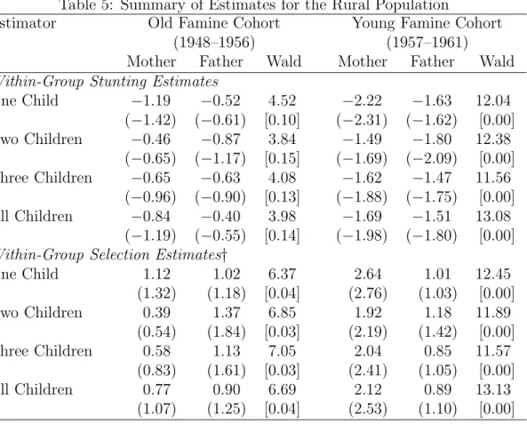
The estimated stunting and selection effects for the rural sample are presented in Ta-ble 5. As discussed in Section 5, issues of multicollinearity between the mother’s and the father’s cohort dummies render t-tests unreliable and hence Wald tests are used to test statistical significance. It is possible that families with many children living at home are an unrepresentative group, and we therefore report results for four different specifications
18As a consequence combining the parents’ equations, certain parameters are no longer separately
related to the number of children used in the estimation.19
As predicted by our preliminary analysis, we find large and significant stunting of the young famine cohort for the rural population. For mothers, the estimated stunting effects range from 1.49 to 2.22 cm while for fathers, the estimates are smaller ranging from 1.47 to 1.80 cm. All specifications show joint significance at below the 1% level. The finding of larger stunting effects for mothers is consistent with other evidence that females suffered more than males during the Great Famine (see e.g. Coale and Banister, 1994, and our discussion in Section 2). For the old famine cohort, mothers are stunted between 0.46 cm and 1.19 cm and fathers between 0.40 cm and 0.87 cm.
The estimates are reasonable in comparison with empirical evidence of the immediate impact of drought on height. Hoddinott and Kinsey (2001) find that a year of drought reduced growth of Zimbabwean children aged between 12 and 24 months by between 1.5 and 2.0 cm. However, since they do not follow drought-affected children to full adulthood they do not provide evidence of long-term stunting.
Table 5 also shows estimates of the effect of selection. These are simply calculated as the famine coefficient in the overall OLS regression (Table 3) minus the estimated stunting (Table 5). For the young famine cohort, they are jointly significant at the 1% level. For mothers in the young famine cohort, the estimates range from 1.92 to 2.64 cm while fathers in the young famine cohort show smaller selection of between 0.85 and 1.18 cm. The estimated selection effects for the old famine cohort range from 0.39 to 1.12 cm for mothers and 0.90 to 1.37 cm for fathers, and they are all jointly significant at the 5% level. This suggests that both famine cohorts were positively selected, confirming the empirical evidence reviewed in Section 3.
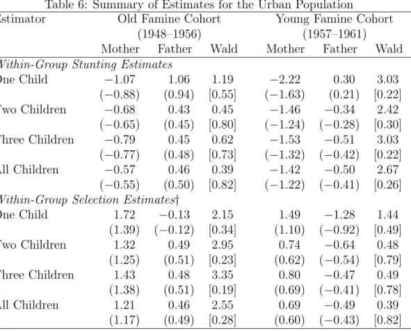
Regarding urban residents, recall that while the old famine cohort appears taller and the young famine cohort shorter than the control group (Table 3), we cannot reject the hypothesis that the children of these cohorts have the same height (Table 4). The esti-mated stunting effects are presented in Table 6. The estimates are negative for the young
19The results are based on all families, but only the first child in each family, the first two children
etc. are used in the estimation. Families with fewer than the maximum number of children are included using standard methods for unbalanced panels.
famine cohort although they are not jointly significant. In the case of the old famine cohort, the estimates are negative only for mothers, but again they are not significant. These findings are consistent with evidence mentioned earlier that urban residents were less affected by the famine.
Our main finding is that the rural young famine cohort are stunted by about 1 to 2 cm and that the selection effect more or less offsets that. Is a 1 to 2 cm height difference important? By way of comparison, we may look at the general relationship between stature and economic conditions. Morgan and Lui (2007) find that from 1937 to 1976 the average male height in Taiwan increased by 1.12 cm per decade. During the 1950s, 1960s and 1970s Taiwan’s per capita real GDP increased by 60, 81, and 97 per cent, respectively. Using China Health and Nutrition Survey data we calculate that the average height of people aged 20 to 25 increased by 2.76 cm between 1997 and 2006. During the same period, Chinese per capita real GDP increased by more than 150% or more than 10 per cent per annum. These figures suggest that a height difference of 1–2 cm could represent very significant differences in economic conditions.
To asses the implications of our estimated selection effects for other populations and other time periods, it is necessary to link selection to child mortality, because evidence from other famines suggests that the majority of people who die during a famine are children. Unfortunately, there are no historical data on the child mortality rate in China during the Great Famine. However, we can construct a very rough estimate using CHNS data for people born immediately after the famine. The average adult height of the males and females born between 1962 and 1966 is 166.85 and 156.22 cm, respectively. If we exclude the bottom 9% of the height distribution for males, the average male height increases by 1.1 cm. Similarly, if we exclude the bottom 20% of the height distribution for females, the average female height increases by 2 cm. This means that if selection operated in a strictly monotone way (e.g. all non-survivors are shorter than all survivors), around 9% of males and around 20% of females must have died to generate selection effects of 1.1 and 2.0 cm, respectively. (Since selection is unlikely to be strictly monotone, these are lower bounds.) As the Chinese famine lasted for 3 years, this translates to average annual
mortality rates of 3% and 6.7% for males and females, respectively. Taking a weighted average for both male and female children, we obtain an average annual mortality rate of 4.9%. Since the majority of people who die during a famine are children, we may further assume that this is also the mortality rate for children aged 0–4.
A child mortality rate of 4.9% during a severe famine is not unusually high. During the Ethiopian famine in 2000, child mortality for those aged 0 to 4 reached 24.8% per annum (e.g. Salama, Assefa, Talley, Spiegel, van der Veen, and Gotway, 2001). During the Bangladesh famine in 1974–1975, the annual mortality rates for infants and children 1–4 years were 16% and 3.5%, respectively (e.g. Chen, Rahman, and Sarder, 1980, Figure 1). These figures suggest that selection effects similar to those we estimate may be relevant in many other developing country settings.
Differences in child mortality are found not only in relation to famines. In a recent cross-country comparison, Bozzoli, Deaton, and Quintana-Domeque (2007) show that even amongst OECD countries, there are large differences in infant mortality rates (e.g. 21 per 1,000 births in Portugal versus 2 per 1,000 births in Sweden). Bhalotra (2007) reports a more than a three-fold difference in the infant mortality rate between the richest and poorest states in India (as mentioned earlier, Deaton, 2008, uses height differences as an indicator of economic inequality in India). There is a potential for selection effects whenever researchers compare height across these populations with such large differences in child mortality.
8
Robustness
Our approach relies on comparing the famine cohorts with people who were either old enough not to be permanently affected by famine or born after the famine. At the same time, we expect average height to increase over the years due to economic progress. The validity of our approach therefore relies on adequately controlling for the time trend. In particular, we are concerned that using the pre-famine control group may lead to an over-estimate of the effects of famine, as the pre-famine control group may have relatively short children. To check the robustness of our estimates, we re-estimate the model dropping
the pre-famine control group. In addition, we re-estimate the model using a “narrow” control group in order to reduce the influence of the time trend. If our results are an ar-tifact of inadequately controlling for birth-year effects, we would expect these alternative definitions to expose such an anomaly.
The results when dropping the pre-famine control group are reported in the Table 7. The OLS results for mother and father’s height (top panel of Table 7) demonstrate a very similar pattern to the full model. In particular, neither of the famine cohorts exhibit any significant visible stunting. Turning to the child-height equation, again the pattern is very similar to the full sample, the young famine cohort has taller children with both the mother and father’s famine cohort dummies being positive and jointly significant. The old famine cohort dummies lose significance, and the sign for the mother’s coefficient in the all-children specification is reversed.
Therefore after excluding the pre-famine control group, there is still no evidence of visible stunting among mothers in the famine cohorts. Moreover, children of young famine cohort continue to be taller than the rest of the sample. If the results for the full sample is an artifact of incorrectly controlling for birth-year effects, one would expect that excluding the pre-famine control group would change the results.20
We next turn to the stunting estimates of this alternative control group (middle panel of Table 7), which yields stunting for mothers in the young famine cohort of between 0.91 and 2.01 cm and between 2.08 to 2.88 cm for fathers in the young famine cohort. These are all jointly significant (p-values of 0.03 or less) and similar in size to the stunting estimates obtained for the full model. For mothers in the old famine cohort we now observe a positive differential for the two-children specification, while fathers show large stunting effects. However, these estimates are individually and jointly insignificant as they were in the case of the full sample.21
20It seems likely that older parents are less likely to have children living at home and it is possible
that this may lead to a bias. The fact that the results are similar when the pre-famine control group is excluded suggests that any bias from only observing sons and daughter who are still at home at the time of the survey is not affecting our results. To be sure, we also estimate the model omitting children 25 years or older. The results are similar.
21Dropping both the pre-famine control group and the old famine cohort yields stunting estimates for
the young famine cohort which are even closer to the estimates on the full sample; however, they are not statistically significant (likely due to the reduction in sample size from 2115 to 869 families).
The narrow control group is defined as those who were born five years immediately before 1948 and five years immediately after 1961. This reduces the sample size from 2115 to 1690 families. The OLS estimates of parental height are reported in the top panel of Table 8. The results indicate that none of the famine dummy variables are statistically significant for either mothers or fathers. The results from the child-height equation are very similar to the full sample. Both famine cohorts have taller children and the coefficients for mothers and fathers are jointly significant.
The within-group estimates of the stunting effects are similar in size to the results using full control group (middle panel of Table 8). Stunting of mothers in the young famine cohort ranges from 1.31 cm to 1.72 cm. For fathers in the young famine cohort, it ranges from 1.89 to 2.16 cm. The young famine cohort continues to be jointly significant. The coefficients of the old famine cohort are not statistically significant.
As yet another check on the results, we estimated the OLS parent- and child-height regressions as well as the within-group model on the full sample, but with a separate dummy for parents born before the famine. We then tested whether the coefficient for the pre-famine control group was significantly different from the post-famine control group. We found that we could not reject the hypothesis of no difference at the 10% level. This suggests that pooling the pre-famine and post-famine control groups is justified.
In the analysis reported in Table 5 we have assumedτm =τf = 1/2, which is reasonable given that there is no evidence in the literature to suggest that the genes of either parent are more important in determining the height of their child. Nevertheless, it is useful to check how sensitive our results are to this assumption. Figure 2 shows the estimated stunting effects and 95% confidence bands plotted against τm (with τf = 1−τm). The solid line is the estimate for the mother and the dashed line is for the father. We only report the two-children specification since one-child and all-children results are similar.22 The figures confirm that the stunting estimates are very robust to changes in τm and τf. The estimates are fairly constant over the range 0.3 to 0.7. This suggests our estimates
22The exponential increase in the width of the confidence band forα
j as τj approaches 0 reflects the
fact that αj is not identified when τj = 0, because the height of the children are not informative about the potential height of the parent in this case.
are robust to variation in gender-specific inheritability of height.
9
Conclusion
This paper estimates the stunting and selection effects of the Great Chinese Famine. The Chinese Famine offers an opportunity for exploring the selection effects of high childhood mortality on adult height. We take a novel approach and develop a powerful econometric model in order to disentangle the stunting from the selection effect of the famine. The model uses the children of the famine cohorts and a control group to identify selection effect. After controlling for selection, we find that rural famine survivors who were exposed to the famine in the first 5 years of life are stunted between 1 and 2 cm. We also find that selection increased the average height of rural female famine survivors by about 2 cm (significant) and the average height of rural male survivors by about 1 cm (insignificant). These findings are robust to alternative definitions of the control group.
As we have argued, the magnitude of the estimated effects are large when taken in context. Furthermore, our rough calculation suggests that the child mortality rate during the Chinese famine is not unusually high compared with other famines. Thus, our findings imply that selection may be an important issue for a wide range of economic studies. The results of this paper therefore suggest that a cautious approach to the use of stature as a measure of well-being in a developing country or historical settings is warranted. While stature undoubtedly has a crucial role to play in documenting economic conditions, interpreting trends in height must be undertaken in light of information on childhood mortality.
A
Technical appendix
A.1
Children’s Age Splines
For children’s height to be a good measure of their genetic height, it is important to control properly for their age. A preliminary data analysis suggested that the population
average height-age relationship for children is very well modeled using cubic splines. For our final results we use
Age1 = 1(age<18) 1 324age 2− 1 9age + 1 Age2 = 1(age<18) 1 864age 3− 1 24age 2+3 8age Age3 = 1(age<10) 27 4000age 3− 27 200age 2+ 27 40age Age4 = 1(age<10) − 1 1000age 3+ 3 100age 2− 3 10age + 1 .
These variables correspond to a cubic spline with knots at age 10 and 18, restricted to be constant after age 18 and restricted to have a continuous first derivative. As defined the variables are scaled to range between 0 and 1. In the estimation we allow for different coefficients for boys and girls.
The splines capture the height-age relationship for children very well, as can be seen in Figure 3 which shows the average age-specific height (circles) and the predicted values obtained from regressing height on the four spline variables and a constant. The variability in the age-specific averages for children in their twenties and thirties is due to small sample sizes.
A.2
Preliminary Estimates Revisited
It is useful to consider the estimates in our preliminary analysis in Section 5 in the light of (8). The parents’ equation (6) is identical to the parents’ equations in (8), if
uijt = gij +ijt. OLS estimation yields inconsistent estimates when (Fij, xijt) and gij are correlated. However, if these variables were uncorrelated the OLS estimator of the stunting, αj, would be consistent, as claimed in Section 5.
The children’s equation (7) is slightly more complicated, because it includes the par-ents’ famine dummies. Suppose there are linear mean relationships between the parpar-ents’ genetic heights on the one hand and the famine dummies and the explanatory variables