REAL TIME OPTIMAL IMPLEMENTATION OF STABILIZING CONTROLLER FOR INVERTED PENDULUM
M. Idi1,2, N. M. Tahir1*, A. G. Ibrahim1,2
1Department of Mechatronics and System Engineering, Abubakar Tafawa Balewa
University (ATBU) Bauchi, Nigeria.
2Faculty of Engineering and Built Environment Glasgow Caledonian University,
Scotland UK
ABSTRACT
This paper present real time control of an inverted pendulum. The system is inherently unstable and multivariable. It is mostly used in laboratories to study, verify and validate new control ideas. The dynamic model of the system was derived based on Lagrange approach and it was linearized. Linear Quadratic Regulator (LQR) controller was designed to stabilize the system in an upright position. The robustness of the control algorithm was tested based on disturbance rejection. Simulation and experimental results showed a good performance was achieved and the controller is robust to external disturbances.
KEYWORDS: Nonlinear; LQR; inverted pendulum;disturbance rejection; Lagrange
1.0 INTRODUCTION
An inverted pendulum is a multivariable, an under-actuated, nonlinear, and unstable system, (Mus & Tovornik, 2006), (Riachy et al, 2007), (Jerome et al, 2013). Due to these dynamics, it is mostly used by researchers to investigate the control algorithms. Modelling and control of the nonlinear inverted pendulum system is one of the major areas of research with lots of potentials in the field of robotics and automation. Various researchers have proposed different control algorithms and techniques for swing up, tracking and stabilization of an inverted pendulum.
Balancing an inverted pendulum mobile robot using LQG and LQR has been proposed by Hauser and Saccon (2005), and their performances were compared. Modelling and a predictive controller based on the nonlinear model of the system have been presented in Chalupa (2008). Similarly, Prasad (2014), Singh and Yadav (2012) and Gupta (2014) compared the stabilization and swing up control performances of LQR and PID controllers for an inverted pendulum. The stabilization control of an inverted pendulum using Pole Placement and LQR has been presented in Kumar et al (2012), a comparison of the control algorithms has also been presented.
Furthermore, an MODE-based optimized LQR developed in Tijani (2013) shows a superior performance. Singh et al (2014) used a modified PSO based PID sliding mode
_________________________________________
for swing up and stabilization control of an inverted pendulum. In addition, Chakraborty et al (2013) investigated the optimization of PID controller using Genetic Algorithm. A dynamic modelling and optimal control of wheel inverted pendulum were proposed in Shamsudin et al (2013) using an optimally tuned partial-state PID. Swing up and stabilization of double inverted pendulum using LQR and LQR based fuzzy was proposed in Bhangal (2013), and their performances were analyzed and compared. An intelligent control algorithm has also been proposed in A-hadithi (2012) and implemented for swing up and stabilization of a double inverted pendulum system. The combinations of intelligent and conventional control have shown good performances and robustness of the control algorithms. An Adaptive Neural Network for motion control of a wheeled, inverted pendulum has also been presented in Yang et al (2014). In Chalupa and Bobal (2008), Model Predictive Controller has been proposed. A novel PSO based Sliding Mode Control for stabilization of an inverted pendulum was presented by Singh et al (2014). In Brisilla and Sankaranarayanan (2015), a stabilization of an inverted pendulum using a nonlinear control algorithm has been presented.
However, to implement a simple control algorithm and obtained stability under external disturbances is a big challenging task. Thus, using LQR the stability and control of all system poles are guaranteed. This paper proposed LQR for real time stabilization of an inverted pendulum under wind disturbances of magnitude of 0.2 N. Time response specification and level of disturbances rejections were used as the performance index of the control algorithms.
2.0 SYSTEM DESCRIPTION
In this part, the inverted pendulum dynamics is presented. 2.1 An Inverted Pendulum System
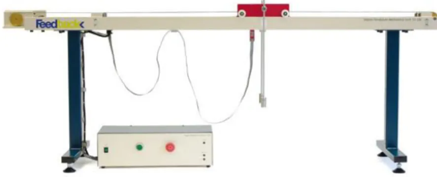
In this work, the laboratory scale feedback digital pendulum system version 33-000-V73 was used. The system consists of the following parts; the cart, two pendulums, a rail, and a D.C motor. The pendulum is hinged at the center of the cart in a manner that they can rotate freely for 360o. The cart can move freely horizontally on the rail with the aid of the D.C motor. The mechanical system is as shown in Figure1.
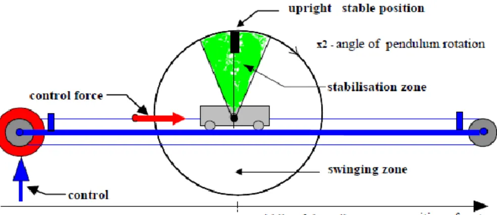
When the pendulum is in the vertical position, the system is unstable and when the pendulum is in a downward position, the system is completely stable. The pendulum is completely unstable for small deviations from the equilibrium position. Figure 2 shows the activity zone of the inverted pendulum within which control can be achieved.
Figure 2. Activity zone of the control algorithm. 2.1.1 System Modelling
The system schematics diagram is shown in Figure 3, with θ, x, and f (t) as pendulum angle, the cart displacement and applied force in (N) respectively. M is the mass of the cart (kg), l is the pendulum length (m), and I is the moment of inertia of the rod from the centre of mass (kgm2). C and b are the translation and viscous damping of the cart (Ns/m) and that of the pendulum (Nm/rad) respectively (Zhang and Tu, 2006).
Figure 3. Schematic diagram of the pendulum-cart system
The energy in the system is simply its kinetic energy and potential energy. The total kinetic energy of the system can be expressed as;
(1)
where T is the total kinetic energy, TM is the kinetic energy of the cart and Tm is the
(2) (3) where V is the velocity of the pendulum’s centre of mass and I is the moment of inertia of the pendulum around the centre of mass and ω is the angular velocity of the pendulum. Also, the position vector can be given as;
(4) And the velocity vector can be express as;
(5) Putting , the kinetic energy of the pendulum becomes;
(6) Hence, the total kinetic energy of the system is as;
(7) In addition, the total potential energy of the system is given as;
(8) where is the potential energy of the cart and is the potential energy of the pendulum. But, VM= 0, and the term Vmis given as
(9) Therefore, the total potential energy can be written as;
(10) The system dynamics equation of motion can be derive using Lagrange’s equation as in Mishra and Chandra (2014).
(11) where, (L) is expressed in form of kinetic energy and potential energy of the system given as;
Substituting T and V in Equation (12), it is obtained as;
(13) Substituting Equation (13) into (11) and solving for the partial derivatives yields;
(14) The above equation can be represented as;
(15)
Moreover, for is given as;
(16) Substituting Equation 13 into 16 and solve for the partial derivatives yields;
(17) Also, Equation 17 can be further simplified as;
(18) After re-arranging, the overall dynamic equations of the system were obtained as;
(19)
2.1.1.1 Model linearization
To linearize the nonlinear system, two points have to be considered for equilibrium points. The pendulum in the upright position (unstable, ) and pendulum in the downward position (stable, ). This can be achieved by Taylor’s series approximation, for a small angle deviation around an equilibrium point ;
(20) Taylor’s series first order approximation is given as;
(21) where , a small angle deviation from equilibrium and higher order neglected. Pendulum in upright position (unstable, ). The following functions can be linearized as
Thus, substituting these into Equation (19), the motion equations were obtained as;
(22)
Pendulum downward position (stable, ). The following functions can also be linearized as;
Thus, the motion Equations were obtained as;
(23)
Hence, the system equations are represented in state space form as;
(24) (25) The states vector of the system can be assigned as;
(26)
where, , are the pendulum angle, angular velocity, Cart displacement and velocity of the Cart respectably (Kizir et al, 2010). Hence the dynamics equations can be represented in state space form as;
(27)
3.0 FULL STATE FEEDBACK CONTROLLER DESIGN
In this section, LQR controller was designed and implemented on real time system. Controllability, observability and stability test was carried out before applying the controller.
3.1.1 Controllability Test
The system is said to be controllable if an input to the plant can take all the states from a desired initial state to a desired final state in a final time interval, otherwise is uncontrollable. Table 1 show the system parameters. The controllability matrix is given as;
(29)
For controllability, the rank (Mc) of the matrix must be equal to the number of states of
the system. Using the MATLAB command, the Mc was obtained to be 4 hence the
system is controllable. 3.1.2 Observability Test
If all states of a system can be determined from an observation of y(t) over a finite time interval, the system is completely observable otherwise is unobservable (Ogata, 1997). The observability matrix is given as;
(30) For observability, the rank (Mo) of the matrix must be equal to the number of the
outputs of the system. Using the MATLAB command, the Mo was obtained as 4 hence
the system is completely observable. 3.1.3 Stability Test
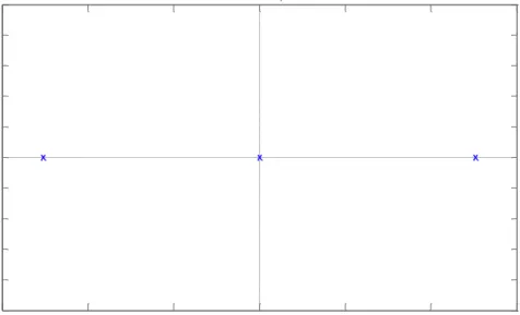
Inverted pendulum system is an unstable system, thus before applying any control algorithms there is need to test the stability of the system before and after control action so that the performance of the controller can be observed. Using the pole zero map
Table 1. System Parameters
Parameter Value
Mass of cart (M) Mass of pole (m) Length of pole (l)
Moment of inertia of the pole (I) Coefficient of friction of cart (b) Damping coefficient of pendulum (d) Gravity (g) 2.4 kg 0.23 kg 0.38 m 0.099 kg/m2 0.05 Ns/m 0.005 Nms/rad 9.8 m/s2
shown in Figure 4, it can be observed that some poles of the system is in the right hand plant hence the system is unstable.
-3 -2 -1 0 1 2 3 -1 -0.8 -0.6 -0.4 -0.2 0 0.2 0.4 0.6 0.8 1 Pole-Zero Map Real Axis Im a g in a ry A xi s
Figure 4. Poles and zero map of the open loop system
3.2 LQR Control Design
The LQR is a full state feedback controller that is usually used in industries for mechanical system control. The control of inverted pendulum using classical PID is mostly difficult because the system has higher state variables than the controller. Hence, as shown in Figure 5, a full state feedback controller is most suitable (Hauser and Saccon, 2005) and (Tahir et al, 2017).
Y K State space model R
-+
XFigure 5. Typical LQR control system
In this control technique, a control law is selected u=( )x to regulate the state x and minimize the performance index:
0 ( ) ( ) ( ) ( ) T T J x t Qx t u t Ru t =
+ (31) where J is the performance index function, are weight matrices for the state variable and control variable respectively. Q and R are the semi-positive definite matrix and semi-positive definite matrix respectively (Ogata, 2010) and(Tahir et al, 2016). Thus, the gain vector K can be obtained to satisfy the feedback control law given as in (Tahir et al, 2017).
(32) where P is the solution of the Riccati equation given as;
(33) In which;
(34) Bryson’s rule states that a first choice of matrices Q and R is to select the matrices diagonals giving by;
(35)
(36)
are the maximum expected value of the state and that of control signal respectively (Lingyan et al, 2009). Therefore, and parameters were used in the following forms;
(37)
(38)
The cart is constrained to lie between and the input to the motor
is constrained to lie between . Thus, , is the
weight due to angle, assuming a 0.2 rad maximum deviation expected from the upright position. , is the weight due to the position of the cart and was assume that the cart should not exceed 0.2m from the centre of the rail. , is the weight due to the control voltage. The close loop controller gain for both simulation and experiment were obtained as K = [58.2411 22.8208 -12.5000 -12.2993] and K = [44.72 200.8 -49.77 -27.38] respectably.
4.0 RESULTS AND DISCUSSION
The real time optimal control implementation of an inverted pendulum was presented. LQR was designed and implemented for swing up and stabilization control of an inverted pendulum. A Gaussian distributed noise and wind disturbance of magnitude 0.2 N was used to test the robustness of the control algorithms in both simulations and experiments respectively..
4.1 Simulation Results
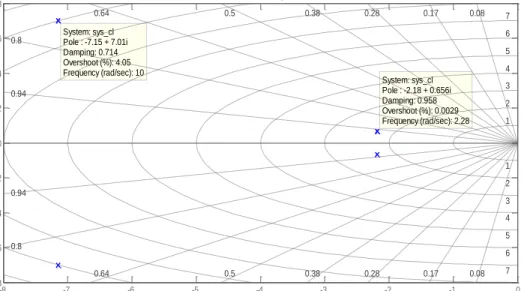
The system is completely stable after applying the controller. Figure 6 shows the poles zeros map of the system, with details of the poles, damping, frequency, and overshoot of the system. Pole-Zero Map Real Axis Im a g in a ry A xi s -8 -7 -6 -5 -4 -3 -2 -1 0 -8 -6 -4 -2 0 2 4 6 8 0.17 0.28 0.38 0.5 0.64 0.8 0.94 1 2 3 4 5 6 7 8 1 2 3 4 5 6 7 8 System: sys_cl Pole : -7.15 + 7.01i Damping: 0.714 Overshoot (%): 4.05 Frequency (rad/sec): 10 System: sys_cl Pole : -2.18 + 0.656i Damping: 0.958 Overshoot (%): 0.0029 Frequency (rad/sec): 2.28 0.08 0.17 0.28 0.38 0.5 0.64 0.8 0.94 0.08
Figure 6. Closed loop poles-zeros map
The cart position, swing angle and control signal of the system were as shown in Figure 7, simulated with an initial condition of 0.1rad. The systems stabilized at 2 sec with 0.262 m undershoot of cart position and 0.08 m of the swing angle.
0 0.5 1 1.5 2 2.5 3 3.5 4 4.5 5 -0.3 -0.2 -0.1 0 0.1 0.2 time [sec] a n g le [ ra d ]/ p o s it io n [ m ] 0 0.5 1 1.5 2 2.5 3 3.5 4 4.5 5 -6 -4 -2 0 2 time [sec] c o n tr o l s ig n a l [v ]
pendulum angle [rad] cart position [m]
control signal [v]
In simulation, a Gaussian distributed noise of mean = 0.0001 and variance = 0.00001 was injected into the control system, at a sampling time of 0.5sec. As shown in Figure 8, the performance of the controller remained the same however, some negligible amplitude and frequency variations can be observed in the system.
0 2 4 6 8 10 12 14 16 18 20 -0.3 -0.2 -0.1 0 0.1 0.2 time [sec] a n g le [ ra d ]/ p o s it io n [ m ] 0 2 4 6 8 10 12 14 16 18 20 -3 -2 -1 0 1 2 time [sec] c o n tr o l s ig n a l [v ]
pendulum angle [rad] cart position [m]
control signal [v]
Figure 8. Disturbance injection response of the system with LQR 4.1.1 Experimental Results
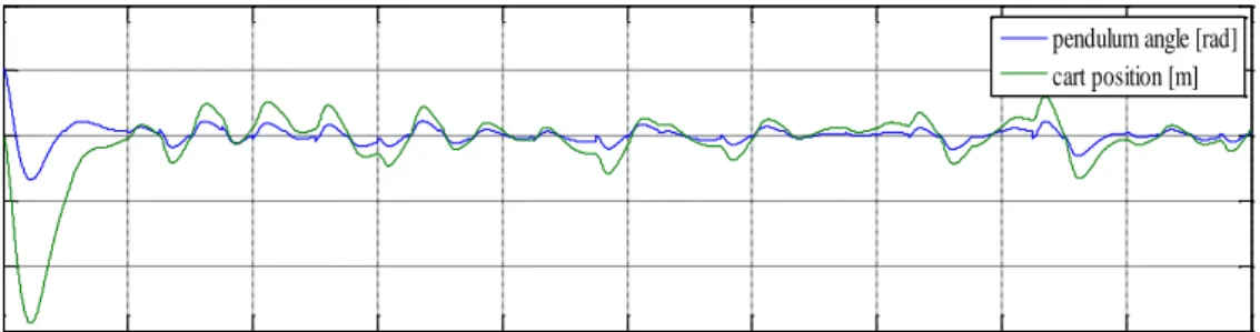
The experiment was conducted at simulation and control laboratory Glasgow Caledonian University UK. Figures 9 and 10 showed the photos of the real time experiment with swing up and stabilizing controller respectably, using the feedback instruments laboratory scale inverted pendulum system.
The algorithm was implemented in real time, the control signal, swing angle, and cart position is as shown in Figure 11, in which the pendula swing up and stabilized within the constraints voltage. It was observed that the controller shows a very good performance as it stabilized the system within the stabilization zone of 0.2 m. A good stabilization and swing up control was also achieved as in Figure 12, with the control action only starting at 13 sec. This is also within the stabilization zone of the system. In addition, the experiment was conducted under a wind disturbance magnitude of 0.2 N and a very good performance was also achieved as shown in Figure 13 but from the control signal it can be observed that under disturbance, more voltage was consumed.
Figure 9. Pendulum in swing-up mode by swinging controller
Figure 10. Pendulum in an upright position controlled by stabilizing controller
0 5 10 15 20 25 30 35 40 -0.4 -0.2 0 0.2 0.4 p o s it io n [ m ] 0 5 10 15 20 25 30 35 40 -2 0 2 4 a n g le [ ra d ] 0 5 10 15 20 25 30 35 40 -5 0 5 10 c o n tr o l [V ] time [s]
0 5 10 15 20 25 30 35 40 -0.4 -0.2 0 0.2 0.4 p o s it io n [ m ] 0 5 10 15 20 25 30 35 40 -2 0 2 4 6 a n g le [ ra d ] 0 5 10 15 20 25 30 35 40 -4 -2 0 2 4 c o n tr o l [V ] time [s]
Figure 12. LQR Swing-up/stabilizing action experimental results
0 5 10 15 20 25 30 35 40 -0.4 -0.2 0 0.2 0.4 p o s it io n [ m ] 0 5 10 15 20 25 30 35 40 -2 0 2 4 6 a n g le [ ra d ] 0 5 10 15 20 25 30 35 40 -5 0 5 10 c o n tr o l [V ] time [s]
Figure 13. LQR Swing-up/stabilizing action experimental results under wind disturbance
5.0CONCLUSION
In this paper, nonlinear inverted pendulum was linearized using Taylor series approach and LQR controller was designed to swing up and stabilize the pendulam. It was also implemented on real time system under wind disturbance. Time response specification and level of disturbances rejection were used as the performance index. Based on
Simulation and experimental results, a very good performance was achieved and the controller is robust to external disturbances. To further reduce the oscillations amplitude and frequencies, enhance and improve the modelling and control for real time accuracies, frictional coefficients should be taking into consideration.
ACKNOWLEDGEMENT
The authors are grateful to Glasgow Caledonian University, Scotland UK and Abubakar Tafawa Balewa University (ATBU) Bauchi, Nigeria for providing financial support and research resources.
REFERENCES
Al-hadithi, B. M. (2012). Fuzzy Optimal Control for Double Inverted Pendulum. 7th
IEEE Conference on Industrial Electronics and Applications. Singapore, 1-5.
Bhangal, N. S. (2013). Design and Performance of LQR and LQR based Fuzzy Controller for Double Inverted Pendulum System. Journal of Image and
Graphics 1(3): 143–146.
Brisilla, R. M. & Sankaranarayanan, V. (2015). Nonlinear control of mobile inverted pendulum. Robotics. Autonomous. Syst., 70: 145–155.
Chakraborty, K., Mukherjee, R. R., and Mukherjee, S. (2013). Tuning Of PID Controller Of Inverted Pendulum Using Genetic Algorithm. International
Journal of Electronics and Communication Technologies, 4(1): 183–186.
Chalupa, P. (2008). Modelling and Predictive Control of Inverted Pendulum.
Proceedings 22nd European Conference on Modelling and Simulation ISBN:
978-0-9553018-5-8.
Chalupa, P., and Bobal, V. (2008). Modelling and Predictive Control of Inverted Pendulum. Proc. 22nd European Conf. Modelling Simulation, 531–537.
Gupta, M. K. (2014). Stabilization of Triple Link Inverted Pendulum system based on LQR control Technique, Recent Advances and Innovations in Engineering. Hauser, J. F. and Saccon, A. (2005). On the Driven Inverted Pendulum, Proceedings the
5th International Conference on Information, Communications and Signal
Processing, Bangkok.
Kizir, S., Bingul, Z. and Oysu, C., (2010). Fuzzy control of a real time inverted pendulum system. Journal of Intelligent and Fuzzy Systems, 21(1-2): 121-133. Ogata, K. (2010). Modern Control Engineering. 5th edition, New Jersy: Prentice Hall.
Lingyan, H., Guoping L., Xiaoping L., and Zhang H, (2009). ThKumar, E. V. and Jerome, J.(2013) Robust LQR Controller Design for Stabilizing and Trajectory Tracking of Inverted Pendulum, Procedia Eng, 64:169–178.
Kumar, P., Mehrotra, O. N., and Mahto, J. (2012). Controller Design Of Inverted Pendulum Using Pole Placement And Lqr, International Journal of Research
in Engineering and Technology 532–538.
Mishra S. K., and Chandra, D. (2014). Stabilization and Tracking Control of Inverted Pendulum Using Fractional Order PID Controllers. Journal of Engineering, 1-9.
Mus N. and Tovornik B. (2006). Swinging Up and Stabilization of a Real Inverted Pendulum, IEEE Transactions on Industrial Electronics, 53(2): 631–639. Prasad, L. B.(2014). Optimal Control of Nonlinear Inverted Pendulum System Using
PID Controller and LQR : IEEE International Conference on Control System,
Computing and Engineering, 11: 661–670.
Riachy S.,Orlov, Y., Floquet, T., Santiesteban R., and Richard. J. (2007). Second-order Sliding Mode Control of Under Actuated Mechanical Systems I: Local Stabilization with Application to an Inverted Pendulum. International Journal
of Robust and Nonlinear Control, 18(4-5). 529-54.
Shamsudin, M. A., Mamat, R., and Nawawi, S. W. (2013). Dynamic Modelling and Optimal Control Scheme Of Wheel Inverted Pendulum for Mobile Robot Application, International Journal of Control Theory and Computer Modelling,
3(6): –20.
Singh, K., Nema, S. and Padhy, P. K. (2014). Modified PSO based PID Sliding Mode Control for Inverted Pendulum, International Conference on Control,
Instrumentation, Communication and Computational Technologies, 722–727.
Singh N. and Yadav, S. K. (2012). Comparison of LQR and PD controller for stabilizing Double Inverted Pendulum System, International Journal of
Engineering Research and Development. ISSN: 2278-067X, 1(12): 69-74.
Tijani, I. B. (2013). Control of an inverted pendulum using MODE-based Optimized LQR controller, IEEE Conference on Industrial Electronics and Applications, 1759–1764.
Tahir, N.M, Hassan,S.M, Mohamed, Z. and Ibrahim,A.G. (2017). Output based Input Shaping for Optimal Control of Single Link Flexible Manipulator, International
Journal on Smart Sensing and Intelligent Systems, 10(2): 367-386.
Tahir,N.M, Bature, A.A, Bature U. I, Sambo A. U, and Babawuro A.Y. (2016). Vibration and Tracking Control of A Single Link Flexible Manipulator Using LQR and Command Shaping. Journal of Multidisciplinary Engineering Science
Yang, C., Li, Z., Member, S., and Cui, R., (2014). Neural Network-Based Motion Control of Underactuated Wheeled Inverted Pendulum Models. IEEE
Transactions on Neural Networks and Learning Systems. 25(11).
Zhang L., and Tu, Y. (2006) Research of Car Inverted Pendulum Model Based on Lagrange Equation. The Sixth World Congress on Intelligent Control and