One-dimensional Bargaining with Markov Recognition Probabilities

P. Jean-Jacques Herings, Arkadi Predtetchinski One-dimensional Bargaining with Markov Recognition Probabilities

RM/07/044 JEL code: C78

Maastricht research school of Economics of TEchnology and ORganizations Universiteit Maastricht

Faculty of Economics and Business Administration P.O. Box 616

NL - 6200 MD Maastricht phone : ++31 43 388 3830 fax : ++31 43 388 4873

One–dimensional Bargaining with Markov Recognition

Probabilities

P. Jean–Jacques Herings

and Arkadi Predtetchinski

October 12, 2007

Abstract

We study a process of bargaining over social outcomes represented by points in the unit interval. The identity of the proposer is determined by a general Markov pro-cess and the acceptance of a proposal requires the approval of it by all the players. We show that for every value of the discount factor below one the subgame perfect equilibrium in stationary strategies is essentially unique and equal to what we call the bargaining equilibrium. We provide a general characterization of the bargaining equilibrium. We consider next the asymptotic behavior of the equilibrium proposals when the discount factor approaches one. We give a complete characterization of the limit of the equilibrium proposals. We show that the limit equilibrium proposals of all the players are the same if the proposer selection process satisfies an irreducibil-ity condition, or more generally, has a unique absorbing set. In general, the limit equilibrium proposals depend on the partition of the set of players in absorbing sets and transient states of the proposer selection process. We fully characterize the limit equilibrium proposals as the unique generalized fixed point of a particular function. This function depends in a simple way on the stationary distribution related to the proposer selection process. We compare the proposal selected according to our bar-gaining model to the one corresponding to the median voter theorem.

JEL classification code: C78.

Keywords: One–dimensional bargaining, Subgame perfect equilibrium, Stationary strate-gies, Markov process.

∗_{Department of Economics, Maastricht University, P.O. Box 616, 6200 MD Maastricht, The}

Nether-lands. E-mail: [email protected] . The author would like to thank the Netherlands Organ-isation for Scientific Research (NWO) for financial support.

†_{Department of Economics, Maastricht University, P.O. Box 616, 6200 MD Maastricht, The}

Nether-lands. E-mail: [email protected] . The author would like to thank the Netherlands Organisation for Scientific Research (NWO) for financial support.

1

Introduction

We consider the situation where a group of players has to choose an alternative out of a set of alternatives represented by points in a one-dimensional space. This problem features prominently in the literature on collective decision making and typical examples concern the choice of the taxation level, the location of a facility, or the amount of money devoted to a particular investment opportunity. A famous solution within this setting is the median voter result (Black, 1958). This result establishes conditions under which the chosen alternative corresponds to the most preferred one by the player with median preferences.

As in Banks and Duggan (2000), Cho and Duggan (2003), Kalandrakis (2006b), and Cardona and Ponsa´ı (2007), we analyze the situation from a bargaining perspective. Prob-lems in collective decision making are often solved by bargaining. Politicians bargain about public good levels, tax rates, and issues in the traditional left–right spectrum in political de-cision making. Within firms bargaining takes place by executives to choose among a variety of investment opportunities. Unions have to aggregate heterogeneous member preferences, which may involve bargaining, and next bargain with firms on terms of employment. Bar-gaining problems within households and committees often lead to a one–dimensional set of alternatives.

Banks and Duggan (2000) consider bargaining over a set of social outcomes equal to an arbitrary compact convex subset of a Euclidean space. They examine a bargaining pro-tocol where the proposer is selected according to a time–invariant probability distribution and they consider a general voting rule that determines whether a particular proposal is accepted or not. They prove the existence of a subgame perfect equilibrium in stationary strategies.

We restrict attention to the case where the set of social outcomes is the unit interval and where acceptance of a proposal requires unanimity of all the players involved in the decision making process. The process by which the proposer is selected follows a general Markov process. The probability by which a certain player is selected as proposer is also referred to as the recognition probability. We would like to emphasize the importance of a general model for the proposer selection process. Romer and Rosenthal (1978) is among the most influential papers emphasizing the role of proposal making on the selected outcome. Kalandrakis (2006a) shows in a bargaining framework that the proposer selection process is more important than voting rights, impatience, or complex equilibrium strategies in explaining political power. Empirical support for this feature in the context of the allocation of transportation funds in the U.S. is provided by Knight (2005).

Two important special cases of our proposer selection model are the ones where the proposer is selected according to some time–invariant probability distribution as in Banks and Duggan (2000) and Kalandrakis (2006b), or where the proposer is chosen according to some deterministically rotating scheme as in Cardona and Ponsat´ı (2007). Also the alternating offer bargaining model in Rubinstein (1982) is an example of a deterministically rotating scheme and is a special case of our more general model. Merlo and Wilson (1995) have generalized the Rubinstein set–up substantially and allow for a proposer selected by

a Markov process. But since they consider bargaining problems where the dimension of the bargaining space equals the number of players minus one, one–dimensional bargaining with more than two players is not covered by their analysis.

The bargaining process we study proceeds as follows. At the beginning of a period one player is determined to make a proposal by means of a Markov process. The players react to the proposal sequentially and can each either accept or reject a proposal. If all players accept, the proposal is implemented, the game ends, and each player receives the payoff of the chosen alternative. Otherwise, the next period begins.

We study subgame perfect equilibria in stationary strategies. In a stationary strat-egy, each player makes a unique history-independent proposal and has a unique proposer-dependent acceptance set. The acceptance set specifies which proposals are accepted by a player. The intersection of all the individual acceptance sets is called the social acceptance set. Like the individual acceptance set, the social acceptance set is proposer-dependent, but otherwise history-independent.

We show that subgame perfect equilibria in stationary strategies are essentially unique. All equilibria have the same equilibrium proposals, the same equilibrium payoffs, and the same social acceptance sets. In equilibrium, proposals are immediately accepted, so in equilibrium no delay occurs. Any two subgame perfect equilibria can only differ with respect to the individual acceptance sets. The difference is only relevant off the equilibrium path and only occurs when a player is indifferent between accepting or rejecting a particular proposal. The unique subgame perfect equilibrium in stationary strategies where players accept if they are indifferent between rejecting and accepting is referred to as the bargaining equilibrium.

Our uniqueness result complements the uniqueness results by Cho and Duggan (2003) and Cardona and Ponsat´ı (2007) in related frameworks, and the uniqueness result in Merlo and Wilson (1998) for the extension of Rubinstein (1982) to then-person case that involves a stochastic cake under a contraction condition. Eraslan and Merlo (2002) show for the latter model that uniqueness does not generally hold when approval of a proposal is not required to be unanimous. Eraslan (2002) obtains a uniqueness result in the legislative bar-gaining approach of Baron and Ferejohn (1989). Kalandrakis (2006b) establishes a number of determinacy results (the number of equilibria is finite, and under some assumptions odd) for a quite general bargaining model.

We continue by studying the asymptotic behavior of subgame perfect equilibrium pro-posals as the discount factor converges to one. As an illustration, consider the special case of time–invariant recognition probabilities. These recognition probabilities give rise to a cumulative distribution function on the set of alternatives, by assigning to each alter-native the mass of players whose most preferred alteralter-native is less than or equal to that alternative. We prove that in the limit the bargaining equilibrium proposals of all players converge to the same proposal, being the (generalized) fixed point of the function equal to one minus the cumulative distribution function.

For the general case, consider a sequence of discount factors converging to one. The induced sequence of bargaining equilibria converges to some limit, which we call the limit equilibrium. It is not necessarily the case that limit equilibrium proposals of players are

all the same. The configuration of limit equilibrium proposals depends on the partition of the set of players into absorbing sets and transient states, based on the proposer selection process. Starting from any transient state, the proposer selection process eventually enters one of the absorbing sets. The probability to enter a given absorbing set starting from a given transient state is called the absorption probability. The proposer selection process determines a unique stationary distribution on each absorbing set. This stationary distri-bution determines a generalized fixed point in a similar way as illustrated for the case of time–invariant recognition probabilities.

The limit equilibrium proposals can therefore be described as follows. (A) Players in the same absorbing set make the same proposal.

(B) The proposal of a player in an absorbing set is the related generalized fixed point. (C) The proposal of a player in a transient state is the weighted average of the absorbing

set proposals, with weights given by the absorption probabilities.

It follows from Conditions (A) and (C) above that if there is only one absorbing set, then all players make the same limit equilibrium proposal. In particular, if the transition matrix of the proposer selection process is irreducible, the only absorbing set is the entire set of players. Also, if the recognition probabilities are time–invariant, the only absorbing set is the set of players with strictly positive recognition probabilities. Condition (B) provides a simple procedure to calculate limit equilibrium proposals. As a particular illustration, we show how the limit equilibrium compares to the median voter theorem, and we argue that it selects less extreme alternatives.

The paper has been organized as follows. Section 2 introduces the model and the no-tion of bargaining equilibrium. In Secno-tion 3 we show that each bargaining equilibrium is a subgame perfect equilibrium in stationary strategies, and conversely that each subgame perfect equilibrium in stationary strategies is essentially a bargaining equilibrium. In Sec-tion 4 we characterize bargaining equilibria by means of a specific system of equaSec-tions and prove that for each value of the discount factor below one there is a unique bargaining equilibrium. Section 5 analyzes bargaining equilibria in a number of special cases, includ-ing the case of time–invariant recognition probabilities and a deterministically rotatinclud-ing scheme of proposers. Section 6 presents two results on stochastic matrices that are needed to show the main result of the paper, presented in Section 7. It fully characterizes the limit equilibrium and its relation to the generalized fixed point of the function generated by the stationary distribution of the proposer selection process. Section 8 concludes the paper.

2

Bargaining Equilibrium

We study an environment where the set of available alternatives or social states is repre-sented by the unit interval. A finite set of players N has to choose one alternative from the set Z = [0,1]. The implementation of an alternative z ∈[0,1] leads to instantaneous payoffs ofui(z) = 1− |z−pi|to player i. Thus pi is the ideal point of player i, and player

i’s payoff decreases linearly with the distance between the ideal point and the alternative. We assume that there are players for which 0, respectively 1, are the ideal points. We use the notationi0 for a player with pi0 = 0 and i1 for a player with pi1 = 1.

Given a discount factor δ ∈[0,1), we define the bargaining game Γ = Γ(δ) as follows. The game Γ is a dynamic game of perfect information. The game starts in periodt = 0. In each period t nature selects a player to make a proposal and the selected player proposes one of the alternatives from Z. Then all players respond to the proposal. Each player can either reject or accept it. The players respond to a proposal sequentially, the order of the responses being history-independent. For simplicity, we assume that all players respond to the proposal, including the proposer himself. If the responders unanimously agree to a proposal, the game ends and the proposal is implemented. As soon as the first rejection occurs, time period t+ 1 begins.

If an alternative z has been implemented in period t, the payoff to player i is δt_u i(z).

The payoff of perpetual disagreement is zero for every player.

The selection of proposers is determined by a Markov process on N. The transition probability from state k to statei is π(i|k). When player k makes a proposal in period t, then with probability π(i|k) player i will be selected to make a proposal in period t+ 1. Transition probabilities are collected in the matrix Π, with π(i|k) in row k and column i

of Π. In period t= 0 the process is initialized by an arbitrary probability distribution on the set N.

Two important special cases of the proposer selection process are time–invariant recog-nition probabilities and deterministic recogrecog-nition rules. Recogrecog-nition probabilities are time– invariant if there is a probability distribution µ on N such that π(i|k) = µ(i) for all (i, k) ∈ N ×N. Recognition is deterministic if there is a function r : N → N such that

π(i|k) equals one if i = r(k) and zero otherwise. The function r is called a recognition rule. When N consists of players i0 and i1 only and recognition is deterministic with the

rule r(i0) = i1 and r(i1) =i0,we obtain the famous model of alternating offers bargaining

of Rubinstein (1982) as a special case.

We will analyze subgame perfect equilibria in stationary strategies. In a stationary strategy a player chooses the same action at information sets with an identical continuation game. A stationary strategy of playericonsists of a proposalxi ∈[0,1] and a collectionAi

of acceptance setsAi|k ⊂[0,1] fork ∈N. The setAi|kis the set of proposals of playerkthat

are accepted by player i. The stationary strategy (xi, Ai) therefore determines a unique

behavioral strategy σi. A stationary strategy profile is a pair (x, A), where x = (xi)i∈N

and A= (Ai)i∈N.

A tuple of acceptance sets A induces the social acceptance set Xk =∩i∈NAi|k, i.e. the

set of proposals by player k that are unanimously accepted. We write X = (Xk)k∈N.

Consider the case where all players make proposals that belong to the respective social acceptance set. Then there is no delay before a proposal is accepted. Such a strategy profile (x, A) is called a no–delay strategy profile. A no–delay strategy profile (x, A) induces a

matrix of continuation payoffs Y with element yi|k in row k and columni defined by

yi|k=

X

j∈N

π(j|k)ui(xj).

The continuation payoffyi|kis next period’s expected instantaneous payoff to playeriwhen

the proposal made by playerk is rejected. Player ishould reject a proposal xk by player k

if ui(xk)< δyi|k. These considerations motivate the definition of a bargaining equilibrium

below.

Definition 2.1 A stationary strategy profile (x, A) is a bargaining equilibrium of Γ if

xk = arg maxz∈Xkuk(z) for each k ∈N, (1)

Ai|k = {z ∈Z|ui(z)≥δyi|k}for each (i, k)∈N ×N, where (2)

yi|k = P_j∈Nπ(j|k)ui(xj) for each (i, k)∈N ×N, (3)

Xk = ∩i∈NAi|k for each k ∈N. (4)

In a bargaining equilibrium no delay ever occurs as all equilibrium proposalsxk lie in the

respective social acceptance setsXk. The numberyi|kis the equilibrium continuation payoff

to player iafter a proposal of player k has been rejected. Playeri accepts a proposalxk of

player k if and only if the instantaneous payoff of xk is at least as high as the discounted

continuation payoff.

3

Subgame Perfect Equilibria in Stationary Strategies

In this section we show that a bargaining equilibrium is a subgame perfect equilibrium in stationary strategies. Moreover, we show the converse result that if (x, A) is a subgame perfect equilibrium in stationary strategies, then there is a bargaining equilibrium where all equilibrium proposals, all social acceptance sets, and all continuation payoffs coincide with those induced by (x, A). As a consequence of the results in this section, we may restrict our analysis of Γ to a study of its bargaining equilibria.

Theorem 3.1 A bargaining equilibrium σ = (x, A) of Γ is a subgame perfect equilibrium in stationary strategies.

We prove Theorem 3.1 in two steps. The first step (Proposition 3.1) is to show that there are no profitable one–shot deviations from the strategy σ at any node of the game Γ. A strategy ¯σi of player i is said to be a one–shot deviation from σ at node h if it

coincides with the strategyσi on all nodes buth. The second step establishes the one–shot

deviation property for the game Γ. The property states that if there is a profitable deviation from a joint strategy σ, then there exists a profitable one–shot deviation. Proposition 3.2 establishes the the one–shot deviation property for Γ.

Proposition 3.1 Let σ = (x, A) be a bargaining equilibrium. Then no player has a one– shot profitable deviation from σ at any node of the game Γ.

Proof. Let ¯σi be a one–shot deviation by player ifrom σ at node h.

Suppose player ihas to make a proposal at nodeh. Under strategyσi playeriproposes

an alternativexi.By the definition of bargaining equilibrium, the proposalxi is an element

of the social acceptance setXi for the proposals of playeri. It is therefore accepted, leading

to a payoff ofui(xi) for playeri. In particular,xi is an element ofAi|i, so thatui(xi)≥δyi|i.

Suppose under strategy ¯σi player i makes a proposal z. If z is not an element of

the social acceptance set Xi for the proposals of player i, it will be rejected. Because ¯σi

coincides with the strategyσi on all nodes followingh, player iwill receive a payoff ofδyi|i.

But since ui(xi) ≥ δyi|i, the strategy ¯σi is not a profitable deviation from σ. If z is an

element of Xi, then z it is accepted and player i receives a payoff of ui(z). However, in

this case ui(z)≤ui(xi), because by the definition of bargaining equilibrium,xi maximizes

the function ui on the set Xi. Again, the strategy ¯σi is not a profitable deviation fromσ.

Suppose that at node h player i has to react to a proposal z of player k. Suppose z is accepted by player i under strategy σi but rejected under strategy ¯σi. Then the strategy

σi leads to a payoff of either ui(z) or δyi|k, depending on whether other players accept or

reject z. Since z is accepted by player i, it is an element of the set Ai|k, so ui(z) ≥ δyi|k.

Because ¯σi coincides with the strategyσi on all nodes followingh, it leads to payoff ofδyi|k

for player i. We see that ¯σi is not a profitable deviation from σ.

Suppose z is rejected by player i under strategy σi but is accepted under strategy ¯σi.

Then the strategy σi leads to a payoff of δyi|k. Since z is rejected by player i, it is not

an element of Ai|k, so ui(z) < δyi|k. The strategy ¯σi leads to payoff of either ui(z) or

δyi|k, depending on whether z is accepted or rejected by other players. Again, ¯σi is not a

profitable deviation from σ.

Proposition 3.2 Letσ be a profile of strategies. If playerihas a profitable deviation from

σ, then player i has a profitable one–shot deviation from σ.

Proof. Given a node h we let t(h) denote the period nodeh belongs to. Suppose player

i has a profitable deviation ¯σi from σ in the subgame Γ(¯h) of the game Γ which increases

the subgame payoff by ε > 0. First we show that there is somer such that player i has a profitable deviation in the subgame Γ(¯h) that coincides with σi on all nodes except those

corresponding to the first r periods of the subgame Γ(¯h).

Since the payoff player i can get in period t is bounded by δt_{, the subgame payoff for}

any strategy that agrees with ¯σi on all nodes corresponding to the first t periods of the

subgame differs from the payoff of ¯σi by at most δt. Set r = ln(ε)/ln(δ) and define the

strategy σr i as follows: σir(h) = ( ¯ σi(h), if t(h)≤r+t(¯h) σi(h), otherwise.

By definition, σr

i coincides with ¯σi on all nodes corresponding to the first r periods of the

subgame Γ(¯h). Therefore, the subgame payoff of σr

i differs from the payoff of ¯σi by δr =ε

at most. It follows that σr

i is a profitable deviation from σi in the subgame Γ(¯h).

Suppose there is a node h in the subgame Γ(¯h) with t(h) =r+t(¯h) such that player i

has to act at h and strategy σr

i is a profitable deviation from σ in the subsubgame Γ(h).

Then σr

i is a profitable one–shot deviation at nodeh. This follows from the fact that each

player acts at most once every period. Thus if node h′ _{follows nodeh and player i has to}

act ath′_{, then t(h}′_{)> r+t(¯h), implying that σ}r

i(h′) =σi(h′). In this case the argument is

complete.

Suppose there is no node h in the subgame Γ(¯h) with t(h) =r+t(¯h) such that player

i has to act ath and strategy σr

i is a profitable deviation in the subsubgame Γ(h). In this

case we define a new strategy for i as follows:

σir−1(h) =

( σr

i(h), if t(h)≤r+t(¯h)−1

σi(h), otherwise.

Then the payoff of σir−1 at any node of the subgame Γ(¯h) is at least as high as the payoff

of σr

i. In particular, σ r−1

i is a profitable deviation from σ in the subgame Γ(¯h). Iterating

this argument, we find a one–shot profitable deviation for player i.

Let σ = (x, A) be a stationary strategy profile in the game Γ. Let Na = {k ∈N|xk ∈

Xk} denote the set of players whose proposal is accepted and Nr = {k ∈ N|xk ∈/ Xk}

denote the set of players whose proposal is rejected. We now compute the matrix Y of continuation payoffs associated with σ. The matrix Y contains yi|k in row k and column

i. If nature chooses a proposer k from the set Na, the payoff to player i is ui(xk), while if

the proposer is chosen fromNr, then the payoff to player iis δyi|k. We have thus a system

of equations yi|k= X j∈Na π(j|k)ui(xk) +δ X j∈Nr π(j|k)yi|j for all (i, k)∈N ×N.

Given a subset S of N let 1S be the vector in RN with each coordinate i∈ S equal to

1 and each coordinatei∈N \S equal to 0. Let Ω(S) be a square matrix with the entries indexed by elements of the set N ×N. The only non–zero entries of Ω(S) are diagonal entries corresponding to the elements of the set S. These entries are equal to one. The matrix Ω(N) is equal to the identity matrix and is also denoted by I. Let u(x) denote the matrix with the element ui(xk) in row k and column i. Then the above system can be

written in the vector–matrix form as

Y = ΠΩ(Na)u(x) +δΠΩ(Nr)Y.

We can now solve for the continuation payoffs:

The matrix [I −δΠΩ(Nr)] is invertible and has a non-negative inverse, because the

spectral radius of δΠΩ(Nr) is at most δ <1. The matrix Λ is therefore non–negative. All

its columns corresponding to players in Nr are equal to zero. The matrix Λ equals the

matrix Π if Nr is empty and has all entries equal to zero if Na is empty.

Furthermore, the sum of the entries of the matrix Λ in any given row is at most 1, that is Λ1N ≤1N. To prove this inequality, consider the following chain of equations:

[I−δΠΩ(Nr)][I−Λ]1N = [I−δΠΩ(Nr)−ΠΩ(Na)]1N = [I−δΠΩ(Nr)−δΠΩ(Na)−(1−δ)ΠΩ(Na)]1N = [I−δΠ−(1−δ)ΠΩ(Na)]1N = 1N −δ1N −(1−δ)Π1Na = (1−δ)(1N −Π1Na) = (1−δ)(Π1N −Π1Na) = (1−δ)Π1Nr.

The equation in the third line follows from the fact that Ω(Na) + Ω(Nr) =I. The equation

in the fourth line uses that Π1N = 1N and Ω(S)1N = 1S. The equation in the sixth

line again uses the fact that Π1N = 1N. The equation in the last line uses the equation

1Na+ 1Nr = 1N.

Premultiplying the obtained equality by the matrix [I −δΠΩ(Nr)]−1 yields

1N −Λ1N = (1−δ)[I−δΠΩ(Nr)]−1Π1Nr,

which is non–negative because [I −δΠΩ(Nr)]−1 is non–negative. This proves that Λ1N ≤

1N.

With λ(j|k) denoting the entry in the row k and column j of the matrix Λ, we can write the continuation payoff as

yi|k =

X

j∈Na

λ(j|k)ui(xj).

Theorem 3.2 Suppose δ ∈[0,1). Let σ = (x, A) be a subgame perfect equilibrium of the game Γ with continuation payoffs Y and social acceptance sets X. Then there exists a bargaining equilibrium (x, B) with continuation payoffs Y and social acceptance sets X.

Proof. Define the following sets:

Bi|k ={z ∈Z|ui(z)≥δyi|k}and Bk =∩i∈NBi|k,

Ci|k={z ∈Z|ui(z)> δyi|k} and Ck =∩i∈NCi|k.

Step 1. We prove that IntBk =Ck ⊂Xk⊂Bk for each k.

To prove the second inclusion let z be an element of Ck. Suppose z is not an element

of Xk. Let i be the last player in the response order such that z is not an element of the

individual acceptance set Ai|k.

Consider any node h of the game Γ where player i has to react to the proposal z of player k. If all players follow the profile of strategies σ, then z is rejected with player i

being the last player in the response sequence to rejectz. Thus under strategyσthe payoff at node h to player iis δyi|k.

Consider a strategy ¯σiof playerithat coincides withσi on all nodes of the game Γ except

nodehwhere it assigns that player iaccept the proposalz. Because all players following i

in the response sequence accept z, playing ¯σi againstσ in the subgame that starts at node

h leads to a payoffui(z) for player i. Since z ∈Ci|k we know thatui(z)> δyi|k. Thus ¯σi is

a profitable one–shot deviation from σ at node h. This contradicts the hypothesis that σ

is a subgame perfect equilibrium.

To prove the third inclusion let z be an element of Xk and supposez is not an element

ofBk. Let ibe any player such thatz is not an element of the setBi|k. Then ui(z) < δyi|k.

Consider any node h of the game Γ where player i has to react to the proposal z of player k. If all players follow the profile of strategies σ, then z is accepted, resulting in payoff ui(z) for player i. Consider a strategy ¯σi for player i that coincides with σi on all

nodes of the game Γ except node h where it assigns that player i reject the proposal z. Playing ¯σi againstσ results in a payoff ofδyi|k for playeri. Thus ¯σi is a profitable one–shot

deviation from σ at node h. This contradiction proves the second inclusion.

Step 2. We prove that the set Ck is non–empty for each k.

Fix some k ∈ N. Let N0 _{= {i ∈ N|y}

i|k = 0} and N+ = {i ∈ N|yi|k > 0}. Since all

utility functionsui are positive on the interior of the unit interval, we have the inclusion

(0,1)⊂ \

i∈N0 Ci|k.

Let λ(N|k) denote the sum of all entries in rowk of Λ. Suppose first that λ(N|k) = 0. Then row k of Λ is zero, and therefore yi|k = 0 for all i∈ N. Thus N0 =N and we have

the inclusion (0,1)⊂Ck. In this case the claim is proven.

Suppose now that λ(N|k)>0. Define the element z of Z by

z =

P

j∈Naλ(j|k)xj λ(N|k) . For each i∈N+ _{we then have the following inequalities:}

ui(z)≥ P j∈Naλ(j|k)ui(xj) λ(N|k) = yi|k λ(N|k) ≥yi|k> δyi|k,

where the first inequality follows from the concavity ofui, the second inequality from the

fact that λ(N|k) ≤1, and the third inequality from the fact that δ <1 and yi|k > 0. We

have thus established the inclusion

z ∈ \

i∈N+ Ci|k.

Each Ci|k is an open subset of Z. Since the set N+ is finite, ∩i∈N+C_i|k is also an open

subset ofZ. As we have just shown, it is a non–empty set. Being a non–empty open subset of Z, it has to have a non–empty intersection with the interior of Z. The result follows.

Step 3. We prove that Na=N.

Suppose not. Take some k in Nr. We show that player k has a profitable one–shot

deviation from σ at any node hwhere he has to make a proposal.

Under strategy σ, player k makes a proposal xk that is rejected, resulting in a payoff

of δyk|k for player k. Take an arbitrary point z in Ck and consider a strategy that agrees

with σk on all nodes of the game Γ except node h, where it assigns that player k make a

proposalz. Since z ∈Ck⊂Xk, the alternative z is unanimously accepted, resulting in the

payoff of uk(z). Since z∈Ck|k, we have the inequality uk(z)> δyk|k. Proposing z at node

h is therefore a profitable one–shot deviation fromσ.

Step 4. We show that xk= arg maxz∈Xkuk(z) for all k∈N.

From Step 3 we know that xk ∈ Xk for all k. If xk does not maximize the function

uk on the set Xk, there exists an alternative z ∈ Xk such that uk(z) > uk(xk). But

then player k has a profitable one–shot deviation from σ at any node h where he has to make a proposal, namely to propose the alternative z. Since z ∈Xk, the alternative z is

unanimously accepted, resulting in the payoff ofuk(z). This contradicts the fact thatσ is

a subgame perfect equilibrium.

Step 5. We show that Xk =Bk for all k∈N.

We know from Step 1 that IntBk ⊂ Xk ⊂Bk. Since Bk is a convex set, the set Xk is

also convex and its closure equalsBk. It is therefore sufficient to show that botha= infXk

and b = supXk are contained in Xk.

From Step 4 we know thatxi0 maximizes the utility functionui0 of player i0 onXk, and xi1 maximizes the utility function ui1 of player i1 onXk. But ui0 is a decreasing function

and ui1 is an increasing function. Thus, we must have that xi0 = a and xi1 = b. This

proves the claim.

Step 6. We prove that (x, B) is a bargaining equilibrium with continuation payoffsY

and social acceptance sets X.

Equations (2) and (4) hold by definition of Bi|k and Bk = Xk. We know from Step 3

that Na = N. Therefore, the matrix Λ equals Π and Y = Πu(x), which is Equation (3).

Step 4 yields Equation (1).

4

A Characterization of Bargaining Equilibria

In this section we show that each game Γ has a unique bargaining equilibrium. Together with Theorems 3.1 and 3.2 of Section 3, this implies that all subgame perfect equilibria in stationary strategies have the same equilibrium proposals, equilibrium utilities, and social acceptance sets.

Herings and Predtetchinski (2007) analyze a one–dimensional bargaining model where players can be clustered in two coalitions, one group having z = 0 as the most preferred

point, the other z = 1. In that special case, there is no need to rely on stationarity of strategies to obtain a similar uniqueness result as in this section, and an analysis of subgame perfect equilibria suffices to obtain the desired result. Within the more general setting of this paper, it is possible to construct examples with multiple subgame perfect equilibria, as is also common in the literature on the extension of the Rubinstein model to the n–player case, see Herrero (1985) and Haller (1986).

Consider a bargaining equilibrium (x, A) with continuation payoffsY and social accep-tance sets X. Since the utility functions ui are concave, all individual acceptance sets are

closed intervals. We shall use the notation [a−_i|k, a+_i|k] to denote the individual acceptance set Ai|k of player i for the proposals of player k. The social acceptance set Xk for the

proposals of player k is also a closed interval, denoted by [x−k, x

+

k].

We now present the two main theorems of this section. Theorem 4.1 is a characteriza-tion of bargaining equilibria by means of a system of equacharacteriza-tions in terms of the equilibrium proposals and the social acceptance sets. Theorem 4.2 states that the bargaining equilib-rium is unique.

The system (5)–(6) below is referred to as the characteristic system of equations.

x−=δΠx, x+ = (1−δ)1N +δΠx, (5) xk =      x− k, if pk ≤x−k, pk, if x−k ≤pk≤x+k, x+ k, if x+k ≤pk, for allk ∈N. (6)

Theorem 4.1 Let (x, A) be a bargaining equilibrium with social acceptance sets Xk =

[x−_k, x+_k]. Then the triple (x, x−_{, x}+_{)is a solution to the characteristic system of equations.}

Conversely, suppose the triple(x, x−_{, x}+_{) is a solution to the characteristic system of}

equa-tions. Then there exists a bargaining equilibrium with x the equilibrium proposal profile and [x−_k, x+_k] the social acceptance set for the proposals of player k.

Theorem 4.2 There exists a unique bargaining equilibrium.

The remainder of the section is devoted to the proof of these two results. If xk is an

equilibrium proposal of player k in a bargaining equilibrium, then it is the point of Xk

closest to the ideal point pk, whence equation (6). To derive Equation (5) we rely on

Propositions 4.1 and 4.2 below. Proposition 4.1 essentially says that the players whose ideal points are 0 and 1 determine all social acceptance sets. Player i1 whose ideal point

is 1 determines the lower endpoint of each social acceptance set, while player i0 with ideal

point is 0 determines the upper endpoint.

Proposition 4.1 Suppose the tuple (x, A, Y, X) satisfies Equations (2), (3), and (4). Let

Ai|k = [a−_i|k, a_i+_|k] and Xk = [x−k, x

+

k]. Then

(b) if pi ≤pj, then x−_i|k≤x_j−_|k and x+_i|k ≤x+_j|k,

(c) the equations x−_k =a−_i1|k and x+_k =a+_i0|k hold, and (d) Xk =Ai0|k∩Ai1|k.

Proof. Claim (a) follows directly from Equation (4). To prove claim (b), notice that

a− i|k = max{0, z − i|k} and a + i|k = min{1, z + i|k}, where

z_i−_|k =pi−(1−δyi|k) and z_i+_|k =pi+ (1−δyi|k).

As max{0,·}and min{1,·}are non–decreasing functions, it is sufficient to show thatz_i−_|k ≤ z_j−_|k and z_i+_|k ≤z_j+_|k whenever pi ≤pj.

For all real z and ˙z the inequality |z| − |z˙| ≤ |z −z˙| holds. Consequently, for each i

and j in N and each z in Z we have ui(z)−uj(z) = |pi −z| − |pj −z| ≤ |pi −pj|, so

|ui(z)−uj(z)| ≤ |pi−pj|. It follows that

|yi|k−yj|k| ≤

X

l∈N

π(l|k)|ui(xl)−uj(xl)| ≤ |pi−pj|.

Now suppose that pi ≤pj. Then

z_i−_|k−z_j−_|k=pi−pj +δ(yi|k−yj|k)≤pi−pj+δ|pi−pj|= (1−δ)(pi−pj)≤0

z_i+_|k−z+_j|k =pi−pj −δ(yi|k−yj|k)≤pi−pj+δ|pi−pj|= (1−δ)(pi−pj)≤0.

Claim (c) follows immediately from (a) and (b). Claim (d) follows from (c) and from the fact that Ai0|k = [0, a

+

i0|k] and Ai1|k = [a

−

i1|k,1].

Proposition 4.2 Suppose the tuple (x, A, Y, X) satisfies Equations (2), (3), and (4). Let

Xk= [x−k, x

+

k]. Then x− =δΠx and x+ = (1−δ)1N +δΠx.

Proof. We already know from Proposition 4.1 that x−k = a

− i1|k and x + k = a + i0|k. Now the

utility function of playeri1 isui1(z) =z. Thusyi1|k = (Πx)k. It follows thata

−

i1|k =δ(Πx)k.

The utility function of player i0 is ui0(z) = 1−z. Therefore, yi0|k = 1−(Πx)k. It follows

that a+_i0|k = 1−δ+δ(Πx)k. The result follows.

Now the proof of Theorem 4.1 is immediate. Suppose (x, A) is a bargaining equilibrium with continuation payoffs Y and social acceptance sets X = ([x−k, x+k])k∈N. Equation (6)

then holds because xk is the point of the social acceptance set [x−k, x

+

k] closest to the point

k. Equation (5) holds by Proposition (4.2). Conversely, suppose the triple (x, x−_{, x}+_{) is a}

solution to the characteristic system of equations. Define Y, A, and X by Equations (3), (2), and (4), respectively, and let Xk = [ ˙x−k,x˙

+

k]. We must show that Equation (1) holds

Equations (2), (3), and (4), Proposition 4.2 implies that ˙x− _{=δΠx and ˙x}+ _{= 1−δ+δx.}

Equation (5) now implies that ˙x− _=x− _{and ˙x}+_=x+_{. Equation (6) implies Equation (1).}

Thus (x, A) is a bargaining equilibrium.

Now we turn to the proof of the uniqueness result. Given i ∈ N and z ∈ Z, let hi(z)

be the point of the interval [δz,1−δ+δz] closest to the point pi. Define the function

F : ZN _{→ Z}N _{by letting F}

i(x) = hi((Πx)i) for each x in ZN. It follows from Theorem

4.1 that x is an equilibrium proposal profile in a bargaining equilibrium if and only if x

is a fixed point of the function F. Proposition 4.3 below shows that the function F is a contraction with respect to the norm on ZN _{given by kxk= max|x}

i|. It then follows that

F has a unique fixed point, thus establishing Theorem 4.2.

Proposition 4.3

(a) For each i∈N, each z and z˙ in Z, |hi(z)−hi( ˙z)| ≤δ|z−z˙|.

(b) For each x in RN, kΠxk ≤ kxk.

(c) For each x and x˙ in ZN_{, kF(x)−F( ˙x)k ≤δkx−x˙k.}

Proof. To prove claim (a) write the function hi as

hi(z) =      1−δ+δz, if z∈Z1 = [0,(pi+δ−1)/δ], pi, if z∈Z2 = [(pi+δ−1)/δ, pi/δ], δz, if z∈Z3 = [pi/δ,1].

The function hi is affine with a slope of δ on Z1 and Z3 and it is a constant on Z2. The

result follows.

To prove claim (b), observe that for each k ∈N we have the inequalities

|(Πx)k|= X i∈N π(i|k)xi ≤ X i∈N π(i|k)|xi| ≤ X i∈N π(i|k)kxk=kxk.

The result follows.

To prove claim (c) we compute

|Fi(x)−Fi( ˙x)| = |hi((Πx)i)−hi((Π ˙x)i)|

≤ δ|(Πx)i−(Π ˙x)i|

= δ|(Π(x−x˙))i|

≤ δkx−x˙k.

5

Some Special Cases

Motivated by Theorem 4.1, we refer to the solution (x, x−_{, x}+_{) of the system 5–6 of}

char-acteristic equations as a bargaining equilibrium.

5.1

Time–invariant recognition probabilities

When the recognition probabilities are time–invariant, the continuation payoffyi|k of player

idoes not depend on the identity of the proposer,k. In particular, a rejection of a proposal by player k leads to the same continuation payoff as a rejection of a proposal by player j. It follows that the individual acceptance set Ai|k of player i for the proposals of player k

does not depend on k. Therefore, also the social acceptance sets Xk do not depend on k

and are all equal to some interval [a, b].

Let µ be time–invariant recognition probabilities. The characteristic system of equa-tions then simplifies as follows:

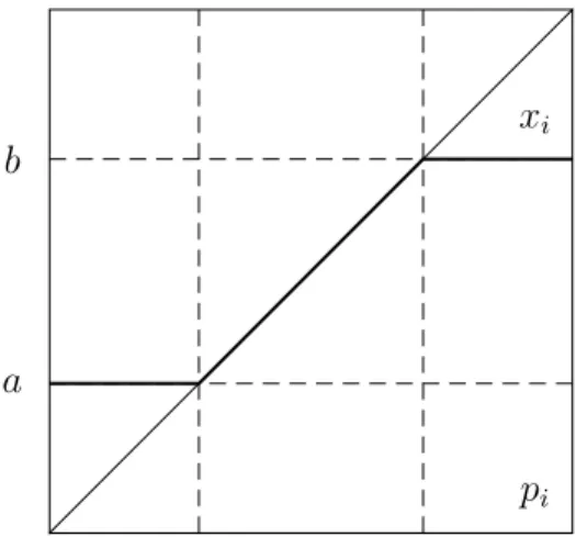
a=δµx, b= 1−δ+δµx, (7) xk=      a, if pk≤a pk, if a≤pk≤b b, if b≤pk, for all k ∈N, (8) where µx=P

i∈Nµ(i)xi. The equilibrium proposals are given by Figure 1 below. Notice

that the equilibrium proposal xi is non–decreasing in pi. An interesting feature of a

bar-gaining equilibrium in the model with time–invariant recognition probabilities is that it is fully characterized by two numbers, namely a and b, the endpoints of the common social acceptance set.

a b

pi

xi

Figure 1: Equilibrium proposal xi in the case of time–invariant recognition probabilities.

Given a discount factorδ ∈[0,1) we let (x(δ), a(δ), b(δ)) denote the unique bargaining equilibrium in a model with time–invariant recognition probabilities µ. The limit of the

bargaining equilibrium asδapproaches one, if it exists, is called the limit equilibrium. Now we compute the limit equilibrium for the case of time–invariant recognition probabilities. In Section 7 we compute the limit equilibrium for the general case.

Definition 5.1 A point z ∈ Z is said to be a generalized fixed point of a non–increasing function f :_R→Z if f(z+ε)≤z ≤f(z−ε) for allε >0.

It is clear that each non–increasing function has at most one generalized fixed point. Define a cumulative distribution function F :R→Z by the equation

F(z) =µ({i∈N|pi ≤z}).

ThusF(z) is the mass of players whose ideal point lie in the interval [0, z]. It is clear thatF

is a non–decreasing function. Theorem 5.1 characterizes limit equilibria as the generalized fixed point of the function 1−F. The proof of the theorem relies on the following result.

Proposition 5.1 Let (x, a, b) be a bargaining equilibrium in a model with time–invariant recognition probabilities. Then 1−F(b)≤µx≤1−F(a).

Proof. Define the elements z− _{and z}+ _{of Z}N _{as follows:}

zi− = ( a, if pi ∈[0, b], b, otherwise, and z + i = ( a, if pi ∈[0, a], b, otherwise.

It is obvious that z− _≤x≤z+_{. Therefore µz}− _≤µx≤µz+_{.Now, we use Equation (7) to}

compute:

µz−=F(b)a+ (1−F(b))b= (1−δ)(1−F(b)) +δµx, µz+ =F(a)a+ (1−F(a))b = (1−δ)(1−F(a)) +δµx.

This yields the desired inequalities 1−F(b)≤µx≤1−F(a).

Theorem 5.1 The limits limδ↑1xi(δ) for i ∈ N, limδ↑1a(δ), and limδ↑1b(δ) exist. All

limits are equal to the unique generalized fixed point of the function 1−F.

Proof. Letδn be a sequence in [0,1) converging to 1. We must show that the sequences

xi(δn) for eachi∈N,a(δn) andb(δn) converge to the generalized fixed point of the function

1−F.

Without loss of generality, assume that the sequences xi(δn) for each i ∈ N, a(δn),

and b(δn) converge. From Equation (7) of the characteristic system for the model with

time–invariant recognition probabilities with know that b(δn) −a(δn) = 1− δn, so the

sequences a(δn) and b(δn) converge to the same limit. Denote this common limit by z.

Sincea(δn)≤xi(δn)≤b(δn) the sequence xi(δn) converges toz for eachi∈N and so does

To prove that z is generalized fixed point of the function 1−F, let ε >0. Then for n

large enough

z−ε≤a(δn)≤b(δn)≤z+ε.

Because F is a non–decreasing function,

F(z−ε)≤F(a(δn))≤F(b(δn))≤F(z+ε).

Applying Proposition 5.1, we find that

1−F(z+ε)≤1−F(b(δn))≤µx(δn)≤1−F(a(δn))≤1−F(z−ε).

Taking the limit we obtain the desired inequality

1−F(z+ε)≤z ≤1−F(z−ε).

The result follows because ε >0 is arbitrary.

As we see from Theorem 5.1, in the model with time–invariant recognition probabilities the common social acceptance set collapses to a point as the discount factor approaches one. As a consequence, the limit equilibrium proposals of all players are the same.

Consider the case where all players have the same probability of making a proposal. We take N sufficiently large and preferences sufficiently dispersed, so that for all practi-cal purposes we may assume F is continuous and strictly increasing. The median voter result states that the group of players selects the alternative zm satisfying F(zm) = 1/2.

According to Theorem 5.1, the alternative zb satisfying zb+F(zb) = 1 is chosen in our

limit equilibrium. The alternatives zm and zb are the same and equal to 1/2 if and only

if F(1/2) = 1/2, i.e. the median voter’s most preferred outcome is 1/2. If F(1/2)<1/2, then it follows that zm > zb ≥1/2, and ifF(1/2)>1/2, then zm < zb ≤1/2.

The median voter outcome is more extreme than the outcome selected in our bar-gaining model. The underlying intuition is that the barbar-gaining model requires unanimous agreement and therefore also the agreement of both the players i0 and i1. This causes a

tendency to select outcomes in the middle. For the median voter model, the votes of half of the players are sufficient, and the opinion of the other players can be safely ignored.

Most striking is the case where the ideal point of each player is either 0 or 1, µ({i ∈ N|pi = 0}) = (1 +ε)/2 and µ({i∈ N|pi = 1}) = (1−ε)/2 for some ε >0. Then zm= 0

and zb = (1−ε)/2. When ε converges to zero, the median voter outcome converges to 0

and the limit equilibrium outcome to 1/2.

With general Markov recognition probabilities, different proposers face different social acceptance sets. While it is still true that a social acceptance set for the proposal of a given proposer collapses to point, this point is in general different for different proposers and Theorem 5.1 does not simply carry over to the general case.

5.2

Symmetric recognition probabilities

In this subsection we assume thatN ⊂Z and pi =ifor all i∈N. The player setN is said

to besymmetric (around 1/2) if 1−i∈N wheneveri∈N. Suppose N is symmetric. The recognition probabilities Π are said to besymmetric (around 1/2) ifπ(1−i|k) =π(i|k) for alli and k inN.

Proposition 5.2 Assume N ⊂Z and pi =i for all i∈N. Assume the player set N and

the recognition probabilitiesΠ are symmetric. Letx−i =δ/2andx+i = 1−δ/2for all i∈N

and let x be given by Equation (8) with a = δ/2 and b = 1−δ/2. Then (x, x−_{, x}+_{) is a}

bargaining equilibrium.

Proof. We verify that the tuple (x, x−_{, x}+_{) satisfies Equations (5)–(6).}

It is clear from Figure 1 that Equation (6) holds. Since b = 1−a, the function x is symmetric in the sense that x1−i = 1−xi for all i∈N. Therefore, for any k ∈N,

2(Πx)k = X i∈N π(i|k)xi+ X i∈N π(1−i|k)x1−i = X i∈N π(i|k)xi+ X i∈N π(i|k)x1−i = X i∈N π(i|k) = 1,

where the first equality holds because N is symmetric, the second one holds because Π is symmetric, and the third one holds because x is symmetric. We see that Πx is identically equal to 1/2. It follows that Equation (5) holds.

Thus, when N and Π are symmetric, the bargaining equilibrium resembles the one in the case of time–invariant recognition probabilities in that all players face the same social acceptance set. As δ approaches one, the equilibrium proposals of all players converge to 1/2. Notice however, that, unlike the case of time–invariant recognition probabilities, the expected payoffs yi|k and the individual acceptance sets Ai|k depend on k.

5.3

Deterministic recognition rules

Letr :N →N be a recognition rule. Equation (5) can then be rewritten as

x−_i =δxr(i), and x+i = 1−δ+δxr(i) for all i∈N. (9)

Claim (a) of Proposition 5.3 below presents a case where any player, once chosen to be the proposer, remains the proposer for the rest of the game. The result is, not surprisingly, that each player proposes his own ideal point. Claim (b) contains the model of Rubinstein (1982) as a special case. It deals with the case where any player i, once chosen to be the proposer, alternates with player 1−iin being the proposer for the rest of the game.

Proposition 5.3 Assume N ⊂ Z and pi = i for all i ∈ N. Consider a game Γ with a

deterministic recognition rule r.

(a) Let r be the identity. The bargaining equilibrium (x, x−_{, x}+_{) is given by x}−

i = δi,

x+i = 1−δ+δi and xi =i for all i∈N.

(b) Suppose the set N is symmetric around 1/2 and r(i) = 1−i. Let a=δ/(1 +δ) and

b= 1/(1 +δ). Then the bargaining equilibrium (x, x−_{, x}+_{) is given by}

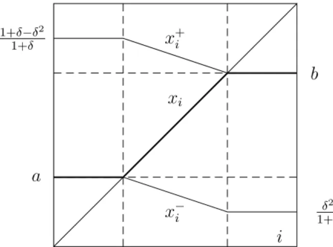
xi =      a, if i≤a, i, if a≤i≤b, b, if b≤i, x−i =      δ/(1 +δ), if i≤a, δ−δi, if a≤i≤b, δ2_{/(1 +δ), if b ≤i,} x+i =      (1 +δ−δ2_{)/(1 +δ), if i≤a,} 1−δi, if a≤i≤b, b, if b ≤i.

Proof. Claim (a) is obvious. Consider claim (b). Figure 2 illustrates the bargaining equilibrium. It is clear from the figure that xi is the point of [x−i , x

+

i ] closest to i, so

that Equation (6) holds. Notice that because b = 1−a, x is symmetric in the sense that

x1−i = 1−xi for all i∈N. Using this property, it is straightforward to verify that

Equa-tion (9) holds as well.

a b 1+δ−δ2 1+δ δ2 1+δ i xi x−_i x+_i

Figure 2: Illustration of x, x− _{and x}+ _{as in claim (b) of Proposition 5.3.}

In part (a) of Proposition 5.3, the equilibrium proposals do not depend on δ.

Figure 2 illustrates the bargaining equilibrium in part (b) of Proposition 5.3. Observe that bothx−_i and x+_i are non–increasing functions ofi. The equilibrium proposalxi is non–

decreasing ini. The equilibrium proposal of each player converges to 1/2 as δ approaches one.

6

Two Results on Stochastic Matrices

This section provides the mathematical results needed to analyze the asymptotic behavior of bargaining equilibria. Given a set S ⊂ N let Sc _{denote the set N \S. Let π(S|i) =}

P

j∈Sπ(j|i).

6.1

Absorbing sets and transient states

The state j is said to lead to state i, written as j →i, if i=j or if there exists a natural number n such that πn_{(i|j) > 0. The states j and i communicate, written as j ↔ i, if}

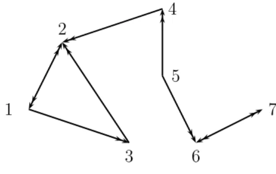
j → i and i → j. The relation ↔ is an equivalence relation. An equivalence class S of the relation ↔ is called an absorbing set if π(S|i) = 1 for all i ∈ S. A state i is said to be transient if it is not an element of any absorbing set. We let A be the collection of absorbing sets andD be the set of transient states. Figure 3 illustrates.

1 2 3 4 5 6 7

Figure 3: Transition probabilities.

There is a double arrow from j to iif theone–stepprobability π(i|j) of transition fromj to i is non–zero. The depicted Markov process has two absorbing sets, {1,2,3} and {6,7}. The states 4 and 5 are transient states. Starting from state 5 there is a non–zero probability to enter either absorbing set, while starting from the state 4 the process enters the absorbing set{1,2,3} with probability 1.

Given a subsetS of N let ΠS denote the restriction of Π to the states inS. Notice that

ifS is an absorbing set, then ΠS is a stochastic matrix, i.e. the the elements in each row of

ΠS add up to 1. A stochastic matrix Π is said to be irreducible if N is the only absorbing

set. If S is an absorbing set, then the stochastic matrix ΠS is irreducible.

Given an absorbing setS, an elementµS ofRS is said to be a stationary distribution on

SifµSΠS =µSandPi∈SµS(i) = 1. By convention,µSis a row vector. For each absorbing

set S there exists a unique stationary distribution onS, see Theorem 4.1 in Seneta (2006). It will be convenient to extend µS to an element of RN by letting µS(i) = 0 for alli∈Sc.

6.2

The convergence of the matrix

Ψ(

δ

)

Ψ = (1−δ)

∞

X

n=0

δn_Πn_{= (1−δ)(I−δΠ)}−1_.

The following is a well–known result.

Theorem 6.1 Let Π be a stochastic irreducible matrix. Let µN denote the unique

sta-tionary distribution on N. As δ approaches one from below, each row of the matrix Ψ(δ)

converges to µN.

We shall use the following straightforward corollary of Theorem 6.1.

Corollary 6.1 Let S be an absorbing set and letµS be the corresponding stationary

distri-bution on S. As δ approaches one from below, each row of the matrix Ψ(δ) corresponding to a state in S converges to µS.

Proof. Define ΨS(δ) by the equation

ΨS(δ) = (1−δ)

∞

X

n=0

δnΠnS.

SinceS is an absorbing set, the matrix ΠS is irreducible, and Theorem 6.1 applies to show

that each row of the matrix ΨS(δ) converges toµS. Now, the elements of the matrix Π are

related to the elements in ΠS by the equation

πn(i|j) =

( πn

S(i|j), if (i, j)∈S×S,

0, if (i, j)∈Sc _×S.

Thus the row j ∈ S of the matrix Πn _{equals the row j of the matrix Π}n

S extended by the

zeros corresponding to states inSc_{. It follows that rowj ∈Sof Ψ(δ) equals rowj of Ψ}

S(δ)

extended by zeros corresponding to states in Sc_{. The result follows.}

6.3

The Perron–Frobenius Theorem and absorption probabilities

We state a version of Perron–Frobenius Theorem for a stochastic irreducible matrix that will be sufficient for our purposes (see Theorem 1.5 in Seneta (2006)).

Theorem 6.2 Let Π be a stochastic irreducible matrix. An element x in RN satisfies the equation Πx=x if and only if it is constant on N.

Using Theorem 6.2 we obtain a characterization of the eigenspace of a general stochastic matrix associated with an eigenvalue one.

Starting from any transient state i ∈ D, the Markov process eventually leaves D and enters one of the absorbing sets where it stays forever. Given an absorbing set S and a transient state i, let ϕ(S|i) denote the probability for the process to enter the set S given the initial statei. Letϕ(S|D) be the column vector of absorption probabilitiesϕ(S|i) as the index i ranges over all transient states. Let π(S|D) be the column vector of probabilities

π(S|i) as the index i ranges over all transient states. The result quoted below combines Theorems 4.3 and 4.4 from Seneta (2006).

Theorem 6.3 Let Π be a stochastic matrix. Then the matrix ID −ΠD is invertible.

Fur-thermore, ϕ(S|D) = [ID −ΠD]−1π(S|D) for each absorbing set S.

The following corollary provides a characterization of the eigenspace of a general stochas-tic matrix Π associated with an eigenvalue one.

Corollary 6.2 Let Π be a stochastic matrix. An element x of RN satisfies the equation

Πx= x if and only if (a) the vector x is constant on each absorbing set, and (b) for each state i∈D

xi =

X

S∈A

ϕ(S|i)xS,

where xS is the value of x on an absorbing set S.

Proof. Suppose Πx=x.

Let S be an absorbing set and let x|S denote the restriction of x to S. It follows that

ΠSx|S =x|S. Since S is an absorbing set, the matrix ΠS is a stochastic irreducible matrix.

By Theorem 6.2, the vector x|S is constant on the set S.

Let xS denote the value of x on S and x|D denote the restriction of x to D. Then the

equations corresponding the transient states can be written as

X

S∈A

π(S|D)xS+ ΠDx|D =x|D.

Solving the system, we obtain

x|D = [ID −ΠD]−1 X S∈A π(S|D)xS = X S∈A ϕ(S|D)xS.

The result follows. The converse direction is now easy to prove.

Consider a Markov process as in Figure 3. If the vector x satisfies the equation Πx = x, then x1 = x2 = x3 and x6 = x7, since {1,2,3} and {6,7} are the absorbing sets of the

process. Furthermore, x4 = x1, because, starting from state 4, the process enters the

absorbing set {1,2,3}with probability 1. Finally, x5 is a convex combination ofx1 andx6

7

The Limit Equilibrium

In this section we study the limit of the bargaining equilibrium when the discount factor tends to one from below. The limit is shown to exist and is called the limit equilibrium. We characterize the limit equilibrium as a generalized fixed point of a particular function. We study under what conditions all players make the same proposal in the limit equilibrium.

Theorem 7.1 below is the main result of the paper. The proof of the theorem relies on Proposition 7.1 below and Corollaries 6.1 and 6.2 in the Appendix.

Given an x ∈ ZN _{let B(x) = {i ∈ N | x}

i < pi}. Notice that B(x) ⊃ B( ˙x) whenever

x≤x˙.

Proposition 7.1 Let (x, x−_{, x}+_{) be a bargaining equilibrium. Then Ψ1}

B− ≤ x ≤ Ψ1_B+

where B−_=B(x+_{) and B}+ _=B(x−_).

Proof. Define the elements z− _{and z}+ _{of Z}N _{as follows:}

z_k−= ( x−_k, if pk≤x+k, x+_k, otherwise, and z + k = ( x−_k, if pk≤x−k, x+_k, otherwise.

Using Equation (6) of the characteristic system, it is easy to see that z− _≤x≤z+_{. Since}

Π preserves the relation ≤, we also have Πz− _≤Πx≤Πz+_{, and, for each naturaln}

Πnz− ≤Πnx≤Πnz+.

Using Equation (5) of the characteristic system, we can rewrite z− _{and z}+ _as

z− =δΠx+ (1−δ)1B− and z

+_{=δΠx+ (1−δ)1}

B+.

Applying Πn _{to each side of the equations, we obtain}

Πnz− =δΠn+1x+ (1−δ)Πn1B− and Π

n

z+ =δΠn+1x+ (1−δ)Πn1B+.

Now we have the following chain of inequalities:

x ≤ z+ =δΠx+ (1−δ)1B+ ≤ δΠz++ (1−δ)1B+ =δ2Π2x+ (1−δ)1_B+ + (1−δ)δΠ1_B+ ≤ · · · ≤ δn+1Πn+1x+ (1−δ) n X i=0 δnΠn1B+.

As n goes to infinity, the first term of the last expression vanishes, while the second term converges to Ψ1B+. We thus obtain the upper boundx≤Ψ1_B+ onx. To obtain the lower

bound, consider the chain of inequalities

x ≥ z−=δΠx+ (1−δ)1B− ≥ δΠz−+ (1−δ)1B− =δ 2_Π2_{x+ (1−δ)1} B−+ (1−δ)δΠ1B− ≥ · · · ≥ δn+1_Πn+1_{x+ (1−δ)} n X δn_Πn₁ B−.

Taking the limit as n goes to infinity, we obtain the lower boundx≥Ψ1B−.

For each absorbing set S define FS :R→Z by lettingFS(z) =µS({i∈S|pi ≤z}). As

FS is a non–decreasing function, the function 1−FS has a unique generalized fixed point.

Definition 7.1 The limit equilibrium is an element of ZN_{, denoted x}ℓ_{, satisfying the}

following conditions: (A) The vector xℓ _{is constant on each absorbing set S, (b) the value}

xℓ

S ofxℓ onS is the generalized fixed point of the function 1−FS, and (C) the value of xℓ

on each transient state iis given by

xℓ i = X S∈A ϕ(S|i)xℓ S. (10)

The conditions (A) and (C) of Definition 7.1 are equivalent to the requirement that Πxℓ ₌

xℓ_{, see Corollary 6.2.}

Given a discount factor δ ∈ [0,1), we let (x(δ), x−_{(δ), x}+_{(δ)) denote the bargaining}

equilibrium.

Theorem 7.1 The limits limδ↑1x(δ), limδ↑1x−(δ), and limδ↑1x+(δ) exist. All three limits

are equal to xℓ_.

Proof. Letδn be a sequence in [0,1) converging to 1. We must show that the sequences

x(δn), x−(δn), and x+(δn) converge to xℓ. Without loss of generality assume that the

sequence x(δn) converges to an element tox of ZN.

The sequence Πx(δn) converges Πx. By Equation (5) of the characteristic system,

x−_(δ

n) = δnΠx(δn) and x+(δn) = (1−δn)1N +δnΠx(δn). It follows that the sequences

x−_(δ

n) and x+(δn) converge to Πx. Since x−(δn) ≤ x(δn) ≤ x+(δn), it then follows that

x(δn) converges to Πx. But we know thatx(δn) converges to x. Thus x= Πx.

We conclude that x is the eigenvector of the matrix Π associated with the eigenvalue one. We now use Corollary 6.2 in Section 6 that provides a complete description of the eigenspace of the matrix Π associated with eigenvalue one. Thus Corollary 6.2 implies that

x is constant on each absorbing set and that Equation (10) holds. It remains to be shown that the value xS of x on each absorbing set S is a generalized fixed point of the function

1−FS.

We already know that the sequences x−_(δ

n) and x+(δn) converge to x. Since N is a

finite set, for n large enough the following inequalities hold:

x−1Nε ≤x−(δn)≤x+(δn)≤x+ 1Nε.

It follows that forn large enough we have the inclusions

B(x+ 1Nε)⊂B(x+(δn))⊂B(x−(δn))⊂B(x−1Nε).

These inclusions imply the inequalities

We then also have the inequalities

Ψ(δn)1B(x+1Nε)≤Ψ(δn)1B(x+(δn)) ≤x(δn)≤Ψ(δn)1B(x−(δn))≤Ψ(δn)1B(x−1Nε),

where the middle inequalities follow from Proposition 7.1.

Now letS be an absorbing set and letxS be the value ofxonS. Letk ∈Sand consider

the inequality

[Ψ(δn)1B(x+1Nε)]k ≤xk(δn)≤[Ψ(δn)1B(x−1Nε)]k.

By Corollary 6.1 in Section 6, row k of the matrix Ψ(δn) converges to µS as n goes to

infinity. We thus obtain the inequalities

µS1B(x+1Nε)≤xS ≤µS1B(x−1Nε).

Now, for any set B ⊂N we have µS1B=µS(B∩S). Furthermore, B(x+ 1Nε)∩S ={i∈

S|xS+ε < pi} and B(x−1Nε)∩S ={i∈S|xS−ε < pi}. Thus, the preceding inequality

can be rewritten as

µS({i∈S|xS+ε < pi})≤xS ≤µS({i∈S|xS−ε < pi}).

The left–hand side equals 1−FS(xS+ε) and the right–hand side equals 1−FS(xS−ε).

Thus we can once again rewrite the preceding inequality as 1−FS(xS +ε)≤xS ≤1−FS(xS−ε).

Since ε > 0 is arbitrary, it follows that xS is the generalized fixed point of the function

1−FS, as desired.

Now we identify some special cases where xℓ _{is constant on the entire player set N. In}

these cases every player makes the same proposal in the limit equilibrium.

Proposition 7.2 If the proposer selection process has a unique absorbing set, then xℓ _is

constant on N.

Proof. The result follows directly from the definition of limit equilibrium. The vector xℓ

is constant on the absorbing set S. Furthermore, starting from each statei outsideS the process is absorbed into S with probability 1, that is ϕ(S|i) = 1.

Proposition 7.3 If the matrixΠ is irreducible, then xℓ _{is constant on N.}

Proof. If the matrix Π is irreducible, then N is the only absorbing set.

Proposition 7.4 Suppose the proposer selection process has time–invariant recognition probabilitiesµ. Then xℓ _{is constant on N and its value is the generalized fixed point of the}

function 1−F, where F(z) =µ({i∈N|pi ≤z}).

Proof. If µare the time–invariant recognition probabilities, thenS ={i∈N|µ(i)>0} is the only absorbing set, and the stationary distribution corresponding toS isµ. The result now follows from Proposition 7.2 and the definition of xℓ_.

8

Conclusion

We have formulated the important problem of how to select an outcome in a one–dimensional set of alternatives as a non–cooperative bargaining problem. We consider the case where a proposal is only accepted if all players approve of it. Subgame perfect equilibrium in stationary strategies is unique up to unimportant details of individual acceptance sets and is called bargaining equilibrium. We provide a simple characterization of the bargaining equilibrium.

In our model, proposers are selected according to a general Markov process. This captures two cases that feature prominently in the literature: the one with time-invariant recognition probabilities and the one with a deterministic proposer selection rule. Our characterization of bargaining equilibrium simplifies further in these important special cases.

Finally, we study the limit equilibrium, the limit of a sequence of bargaining equilibria as the discount factor tends to one. We give an explicit description of the limit equilibrium as the generalized fixed point of a function that is intimately related to the time-invariant distribution of the proposer selection process. Surprisingly, all players make the same proposal in the limit equilibrium under a wide variety of specifications of the proposer selection process.

We may compare the alternative selected in our bargaining model to the one selected according to the median voter theorem. We find that the bargaining alternative is less extreme, i.e. closer to the middle, than the most preferred alternative by the median voter. The bargaining alternative z is the one that satisfies z+F(z) = 1, with F a distribution function related to the players’ most preferred points. The median voter theorem specifies

z such that F(z) = 1/2 as the solution. We have therefore presented a rigorous non-cooperative analysis of the choice of an alternative by a group of players that leads to clear predictions and testable implications.

References

Banks, J.S., and J. Duggan (2000), “A Bargaining Model of Collective Choice,” Amer-ican Political Science Review, 94, 73–88.

Baron, D.P., and J.A. Ferejohn (1989), “Bargaining in Legislatures,”American Po-litical Science Review, 83, 1181–1206.

Black, D. (1958),The Theory of Committees and Elections,Cambridge University Press, London.

Cardona, D., and C. Ponsat´ı (2007), “Bargaining One–Dimensional Social Choices,”

Journal of Economic Theory, forthcoming. doi: 10.1016/j.jet.2006.12.001.

Cho, S.-J., and J. Duggan (2003), “Uniqueness of Stationary Equilibria in a One– Dimensional Model of Bargaining,” Journal of Economic Theory, 113, 118–130.

Eraslan, H. (2002), “Uniqueness of Stationary Equilibrium Payoffs in the Baron-Ferejohn Model,” Journal of Economic Theory, 103, 11–30.

Eraslan, H., and A. Merlo (2002), “Majority Rule in a Stochastic Model of Bargain-ing,” Journal of Economic Theory, 103, 31–48.

Haller, H. (1986), “Non-cooperative Bargaining of N ≥ 3 Players,” Economic Letters, 22, 11–13.

Herings, P.J.J., and A. Predtetchinski (2007), Sequential Share Bargaining, ME-TEOR Research Memorandum 07/005, Maastricht University, The Netherlands.

Herrero, M. (1985), A Strategic Bargaining Approach to Market Institutions, PhD The-sis, London School of Economics, London.

Kalandrakis, T. (2006a), “Proposal Rights and Political Power,” American Journal of Political Science, 50, 441–448.

Kalandrakis, T. (2006b), “Regularity of Pure Strategy Equilibrium Points in a Class of Bargaining Games,” Economic Theory, 28,309–329.

Knight, B. (2005), “Estimating the Value of Proposal Power,” American Economic Re-view, 95, 1639–1652.

Merlo, A., and C. Wilson (1995), “A Stochastic Model of Sequential Bargaining with Complete Information,” Econometrica, 63, 371-399.

Merlo, A., and C. Wilson (1998), “Efficient Delays in a Stochastic Model of Bargain-ing,” Economic Theory, 11, 39–55.

Romer, Th., and H. Rosenthal (1978), “Political Resource Allocation, Controlled Agen-das, and the Status Quo,” Public Choice, 33, 27–44.

Rubinstein, A. (1982), “Perfect Equilibrium in a Bargaining Model,”Econometrica, 50,

97–109.

Seneta, E. (2006),Non–negative Matrices and Markov Chains,Series in Statistics, Springer-Verlag, Berlin.