Spatial Aggregation and Weather Risk Management

Spatial Aggregation and Weather Risk Management

Joshua D. Woodard and Philip Garcia

University of Illinois at Urbana-Champaign Correspondence: [email protected]

Selected Paper prepared for presentation at the American Agricultural Economics Association Annual Meeting, Portland, OR, July 29-August 1, 2007

Copyright 2007 by Joshua D. Woodard and Philip Garcia. All rights reserved. Readers may make verbatim copies of this document for non-commercial purposes by any means, provided that this copyright notice appears on all such copies.

Spatial Aggregation and Weather Risk Management

Abstract

Previous studies identify limited potential efficacy of weather derivatives in hedging agricultural exposures. In contrast to earlier studies which investigate the problem at low levels of aggregation, we find using straight forward temperature contracts that better weather hedging opportunities exist at higher levels of spatial aggregation. Aggregating production exposures reduces idiosyncratic (i.e. localized or region specific) risk, leaving a greater proportion of the total risk in the form of systemic

weather risk which can be effectively hedged using weather derivatives. The aggregation effect suggests that the potential for weather derivatives in agriculture may be greater than previously thought, particularly for aggregators of risk such as re/insurers.

Keywords: weather derivatives, spatial aggregation, corn, yield risk, crop insurance,

Spatial Aggregation and Weather Risk Management

The failures of crop insurance markets in the form of high loss ratios, low participation rates, and the aversion of private insurance companies to bearing exposures have been documented extensively. Early explanations attributed these failures primarily to

information asymmetries related to moral hazard and adverse selection (Chambers 1989; Skees and Reed 1986; Nelson and Loehman 1987; Goodwin and Smith 1995; Gardner 1994; Just and Calvin 1994; Quiggen 1994; Quiggen, Karagiannis and Stanton 1994).1 More recently, a different view has gained support that relates market failures to the inherent systemic nature of the risks in insuring agricultural production (Miranda and Glauber 1997; Duncan and Meyers 2000; and Mason, Hayes and Lence 2003).

Systemic risk in agricultural insurance markets stems from spatially correlated adverse weather events. Research on this explanation concentrates primarily on

identifying the nature and magnitude of systemic risks (Mason, Hayes and Lence 2003; Miranda and Glauber 1997) and on investigating ways in which the risks can be managed utilizing private reinsurance and capital markets (Hayes, Lence and Mason 2004; Turvey, Nayak and Sparling 1999; Miranda and Glauber 1997). To date, no empirical

investigation of reinsurance hedging with weather derivatives (WDs) has been conducted A key characteristic of agriculture is that it is extremely weather sensitive, and the use of WDs in agriculture has received increased attention recently. Currently, the WD market is the fastest growing derivative market in the world (Brockett, Wang and Yang 2005). According to the Chicago Mercantile Exchange (CME) the value of CME Weather products grew nine fold in the first nine months of 2005, growing from $2.2

billion in 2004 to $22 billion through September 2005, with trading volume surpassing 630,000 contracts. While numerous authors have suggested the potential of weather hedging in a reinsurance context on conceptual grounds (Glauber 2004; Skees and Barnett 1999), earlier research suggests that the potential effectiveness of WDs at the farm level may be limited (Vedenov and Barnett 2004). Evaluation at low levels of aggregation, however, may not be relevant for re/insurers who are exposed to more aggregated risks, but no clear explanation has been offered to clarify why one might expect improved WD hedging performance at the re/insurance (i.e. aggregate) versus the primary (i.e. farm) level.

This study attempts to bridge these gaps in the literature by proposing that WD hedging may be more effective at higher levels of aggregation. Specifically, aggregating production exposures across space may reduce idiosyncratic (i.e. localized or region specific) risk in the aggregate portfolio. A greater proportion of the aggregate portfolio’s total risk may be left in the form of systemic weather risk relative to idiosyncratic risk, which may be effectively hedged using WDs. A conceptual model that supports this notion is developed. The hypothesis is investigated at varying levels of aggregation using Illinois corn during 1971-2002 at the CRD and state level.

The hedging analysis assumes minimization of semi-variance. The expected-shortfall measure of tail-risk is also evaluated. These measures of downside risk are more relevant to re/insurers, as they are typically more concerned with loss events. The hedging analysis focuses on seasonal temperature derivatives in lieu of more complex monthly precipitation and temperature derivatives used in previous studies for several reasons. The interaction of temperature and precipitation during loss events, temperature

autocorrelations, and high computation costs limit the potential benefits of more complex WDs. Also, transaction costs associated with negotiating over-the-counter (OTC)

precipitation derivatives are likely high, and their potential for liquidity low, relative to temperature derivatives. Further, the markets for the temperature derivatives traded at the CME are currently the most developed WD markets. The WDs employed here, which are highly consistent with the CME contracts in structure, thus appear to present a promising avenue for current research.

Weather Risk in Crop Insurance Markets

In contrast to earlier studies on failures in crop insurance markets, Miranda and Glauber (1997; hereafter MG) propose that systemic weather risk poses a serious obstacle to the emergence of independent private crop insurance markets because widespread adverse weather induces significant correlations among individual farm-level yields. MG

estimate that US crop insurer portfolios are between twenty to fifty times riskier than they otherwise would be if yields were independent. Thus, the lack of independence among individual yields causes crop insurers to bear substantially higher risk per unit of premium than other property liability and business insurers.

In order to induce insurers to underwrite crop insurance, insurers in the United States are provided reinsurance protection by the government under the Standard Reinsurance Agreement (SRA). The SRA imposes large administrative costs on the public. Further, the extent to which the SRA effectively transfers systemic risks from the

insurer to the government is not known. Ineffective transfer of systemic risk under the SRA may impose additional costs on the government if insurers do not have the

incentives to appropriately monitor the policies they underwrite. Also, the current structure of the SRA is restrictive in terms of how insurers may price the policies they underwrite. All of these factors contribute to excess costs, whether implicit or explicit, generated by the absence of competitive and independent agricultural insurance markets.

MG suggest that area yield reinsurance contracts may permit crop insurers to cover most of their systemic crop loss risk, reducing their risk exposure to levels typically experienced by conventional property liability insurers.2 Given the ability to hedge their systemic risk, crop insurers may be less averse to insuring crop production independently, lessening the need for government intervention and increasing the efficient functioning of agricultural insurance markets.

Hayes, Lence and Mason (2004), 3 as well as MG (1997), investigate the effectiveness of area yield derivatives in hedging crop insurance risk. Although area yield contracts did trade for a short time in an exchange setting, they eventually failed due to insufficient trading volume. A major problem was that market-makers were largely uninterested in taking the other side of such specialized contracts because they were unable to offset the resulting risk. This does not appear to be the case for weather derivatives. The potential for liquidity in WD markets is greater due to the number of market agents with naturally opposing hedge preferences (e.g., electrical utilities).

Hayes, Lence and Mason (2004) also investigate the hedging effectiveness of price derivatives. The primary risk factor in crop insurance, however, is not price but rather widespread adverse weather events such as drought and extreme temperatures during critical growing periods. In addition, plant disease and infection can be intensified by adverse weather.

While researchers have suggested that WDs may be useful for hedging systemic risk, the use of WDs by producers is questionable. For example, Vedenov and Barnett (2004; hereafter VB) analyze the efficiency of WDs as primary hedging instruments for corn, soybeans, and cotton in the U.S. at the CRD level of aggregation. Based on relatively complex non-linear combinations of monthly (June, July, and August) precipitation and temperature indexes, VB’s results suggest only the limited efficacy of WDs in hedging disaggregated production exposures.4

This study builds on earlier research in two important dimensions. First, hedging effectiveness of WDs are investigated at varying levels of spatial aggregation (i.e., the state and CRD level). Yields evaluated at low levels of aggregation (e.g., farm or CRD level) are likely much riskier than those at higher levels (e.g., state level) because the potential degree to which idiosyncratic risks self-diversify increases as the level of aggregation increases. Yet, high temperature spatial correlations induce significant correlations among low-level yield exposures. Thus, relatively more risk may be left in the form of systemic weather risk and the hedging effectiveness of WDs may increase as the level of aggregation is increased. Analysis of aggregated yields may also be more relevant from the re/insurers viewpoint as aggregate yield risk more accurately embodies their systemic risk.

Second, we investigate straight forward seasonal temperature WDs in lieu of complex monthly temperature and precipitation WDs. Persistence in weather conditions may induce a high degree of collinearity among precipitation and temperature (Namias 1986). This, along with the fact that weather conditions in the U.S. during the summer tend to be autocorrelated (Jewson and Brix 2005), increases the probability of

misspecifying weather hedges that involve multiple underlying indexes. The current work simplifies the analysis by investigating seasonal (June, July, and August) temperature WDs.

Conceptual Model

Idiosyncratic effects may self-diversify when aggregated, leaving a greater proportion of the total risk in the form of weather risk. Thus, WD hedging may be more effective for aggregate rather than disaggregate yield exposures. The magnitude of the spatial

aggregation effect depends on the relative correlations of weather and idiosyncratic yield effects across locations. To illustrate, assume yields can be decomposed into two effects, weather effects,W, and all other effects,ε, which may be correlated. Consider a simple model of crop yields which allows for non-linear terms

(1) Y_{t k,} =α_k+ f_k(W_{t k,} )+ε_{t k,}

where t is the time index, k is the location index, is a vector of weather variables,

represents the systemic weather component of yields, , t k W , ( k t k f W ) ε_{t k,} represents the

idiosyncratic risk component, and E[ε_{t k,} ] 0= . Summing across k locations, gives

(2) [ t k_, ] k [ k( t k_, )] [ t k k k k k E

∑

∑

∑

∑

Var

∑

∑

∑

∑

∑

then, as the individual yields are summed, more variation in yields may be able to be attributed to the weather effects at larger levels of spatial aggregation. Thus, WD

hedging may be more effective at larger levels of spatial aggregation.

To illustrate consider an extreme case. Suppose there are two locations and that the ε_{t k,} 's are perfectly negatively correlated, f_k(W_{t k,} ) 's are perfectly positively

correlated, andCov f[ (_k W_{t k,} ),ε_{t j,} ] 0= ∀j k, . In this case the variance of aggregate yields reduces t (4) o [ t k_, ] [ k( t k_, )] k k Var

∑

∑

and all variation in yields can be attributed to weather events. This risk can be potentially

e

y not be useful for individual

tors of

y not always be the case. At the other extreme, consider two location

hedged with a WD equal in size but opposite in direction to the underlying systemic weather effect, f W_k( _{t k,} ). This situation is depicted in Figure 1. If W can be

approximated by erature index the risk of the aggregated expo re can b effectively hedged with a call option on the index Wwith strike price K*. This

framework supports the notion that while WDs ma

producers they may still prove useful in hedging systemic risks borne by aggrega risk such as re/insurers.

Of course, this ma

a temp su

s where the ε_{t k,} 's are perfectly positively correlated, the f_k(W_{t k,} ) 's are perfect

negatively correlated Cov f[ (_{k t k,} ), _{t j,} ] 0 j k,

ly

, and W ε = ∀ . In this riance of

aggregate yields reduces to (5) case the va ] , , [ t k] [ t k k k Var

∑

∑

While both cases are unrealistic they illustrate the main point of the aggregation all variation in aggregate yields is attributed to idiosyncratic effects and none of the aggregate risk can be hedged using WDs.

argument. If weather events across locations are highly correlated, but other yield effects are rela

e ields should have a diversifying effect a

Failure to account for technological advancements in crop production can produce rical yields may produce spurious

ed as

tively less correlated, then relatively more variation (i.e. risk) in yields can be attributed to weather events as yields are aggregated. Empirically, the relevant question for the re/insurer is whether the differences in the correlations of weather effects and other yield effects are significant enough to see substantial differences in WD hedging effectiveness as the level of aggregation increases.

There are good reasons to believe that WD hedging may be more effective as th level of aggregation is increased. First, aggregating y

cross locations. Popp, Rudstrom and Manning (2005), for instance, find that the risk of farm-level yields is substantially higher than county-level yields. This is partly due to the diversifying effect as yields are aggregated over individual farms.5 Second, weather events tend to be highly spatially correlated.6 For example, the average

correlation between the temperature indexes used in this study (the temperature indexes are described in section 5) across locations was 0.755.7

Yields, Weather Indexes, Derivatives, and Pricing

misleading hedging results. Significant trends in histo

hedge ratios which are not representative of the underlying optimal hedge ratio distribution. To account for changes in technology district level yields are detrended using a simple log-linear trend model (VB 2004)8

(6) log(Y_ttr)=α₀ +α₁(t−1971), t =1971,1972,...,2002. Detrended yields to 2002 equivalents are calculat

(7) det ₌ 2002, ₌1971,...,2002 t Y Y Y Y _tr t tr t t

where are observed yields and are the corresponding yield trends.

The negative effect of temperature stress on corn yields during the summer season

in l 1994; Tiegen 1991; a e he D’s for e t Y Y_ttr

is well accepted (see, e.g., Monjard o, Smith and Jones 2005; Dixon et a

nd Kaufmann and Snell 1997). Furthermore, temperature derivatives are likely the most feasible weather variable on which to structure weather contracts from a transaction cost standpoint. Thus temperature derivatives are adopted for this study. Th temperature variables used are Accumulated Cooling Degree Days (ACDD’s) for t summer season: June, July, and August. Agronomic experiments indicate that cooling degree days (CDD’s) are more relevant to crop yields than outright temperature measurements (Schlenker, Hanemann and Fisher 2006). Further, the temperature derivatives traded on the CME are written on ACDD indexes. The number of CD a single day is defined as the amount by which the average temperature is above th reference temperature, sixty-five degrees Fahrenheit. Explicitly, the number of CDD’s on any day t is given by

(8) CDD_t =Max(0,T_t −65)

where T_t is the average temperature on day t. The average temperature is the simple

aximum and minimum

N M t

arithmetic average of the daily m temperatures. The index of ACDD’s on any date, t, is simply defined as

(9) MN =

∑

t CDD

ACDD , , t=M −N,...,M −

=

Although precipitation is also an important risk factor in crop yields, we restrict analysis to temperature derivatives due to the higher potential for liquidity in temperature

derivat e

86). In

four of

ct that

y tradable s are systemically related to summer ACDD’s, there is

derivatives. For instance, from October 14, 1997 to April 15, 2001, temperature

ives represented over 98% of all WDs (Brockett, Wang and Yang 2005). The us of temperature derivatives may not be a major shortcoming as atmospheric flow patterns that control much of the North American climate tend to be persistent (Namias 19

particular, during extreme drought events—those most likely to result in widespread crop losses—this persistence phenomenon causes heat and precipitation conditions to interact causing a self-perpetuating event. On a large scale, average temperature and precipitation conditions for a given region are likely highly negatively correlated in extreme events.

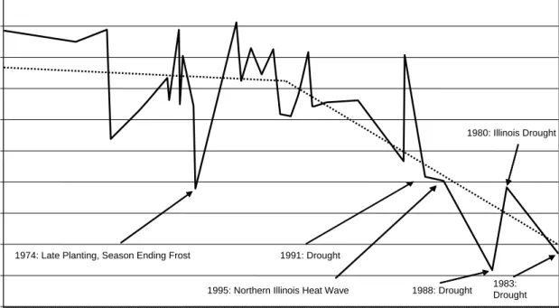
Figure 2 displays aggregate detrended Illinois state corn yields for 1971-2002, with the x-axis ordered by summer season ACDD’s. The hottest years, those in which

ACDD’s exceeded approximately 900, corresponded roughly to the driest years. In fact, the five hottest years were also drought years. Furthermore, all droughts

corresponded to temperatures in excess of 900 ACDD’s. Thus, it appears that

temperature derivatives may act as a suitable substitute in hedging precipitation risk when it is most needed. The use of an accumulated index is further motivated by the fa

in the U.S. corn growing regions, month-to-month temperatures are typically autocorrelated (Jewson and Brix 2005).

Hedging yield risk with WDs becomes a difficult problem for two reasons. First, there is a high degree of yield variability that cannot be attributed to potentiall

weather indexes. For instance, while yield

example, large yield shortfalls may be due to other events not related to ACDD’s, such as in 1974 when late planting and an early season-ending frost were responsible for lar yield shortfalls (Figure 2). Second, the relationship between weather and yields is likely non-linear. In Figure 2 a trend line is obtained by plotting the fitted values from

regressing yields on ACCD’s for the highest (above 900) and lowest (below 900) observed ACCD’s separately. For Illinois corn, it appears that yields are non-linearly related to ACDD’s, suggesting the potential advantage in hedging applications of a options contract which can be non-linearly related to an ACCD index. In the analysis w include swaps as well as options in order to investigate the degree to which non-linea weather effects exist in yields.

All derivatives are priced using burn analysis (BA). BA is the simplest method for pricing weather derivatives, a

ge

n e r

nd is based on calculating what the contract would have paid ou

)

t in the past based on observed historical distributions.9 It is attractive in that it does not require strong assumptions about the distribution of the underlying index, and it is simple to compute.10

The pay-off, f, from a long swap contract is given by

(10) f ACDD( )=D ACDD( −K

where A CCD, and K is the strike

tract pays $D per ACCD ab

. If e

CDD is the index, D is the tick value measured in $/A

price of the contract (i.e. the con ove the chosen strike price

K). The pay-off is a linear function of the index. The buyer is swapping a certain

exposure, K, to the index for an uncertain exposure, ACDD, and thus the name swap.

Most swaps are costless (i.e. there is no premium, and the pay-off equals the profit) the swap contract is to be traded without a premium then the strike must be set at a valu

such that the expected pay-off is zero, that is KF = E(ACDD), where KFis known as the “fair strike”. Pricing of a swap thus entails determining the fair strike. Pricing a zero-cost linear swap using BA simply involves setting the fair strike equal to the historical average of the index.

))

11

The pay-off, p, from a long call option is given by

(11) p ACDD K( , )=Max(0, (D ACDD−K and the

ACDD K Max D ACDD K

profit, π, is given by

(12) π ( , )= (0, ( − ))−P K( )

r premium. For options, pricing entails simply determining ir price which is defined so that the expected pr

and Risk Measures

ollowing VB, the hedge ratio is determined by minimizing the semi-variance (SV) of a SV only measures deviations below the mean where P is the option price, o

the fair premium, or fa ofit on the contract

is zero. The fair price is equal to the expected pay-off of the contract, or P = E(p), and

pricing using BA simply consists of calculating the mean of the historical pay-offs, p,

given a strike, K.

Hedging Analysis F

portfolio consisting of yields and a WD.

and thus is a measure of downside risk. Formally, for swaps the weight, or hedge ratio (contracts/acre), w, is chosenby solving

(13) det 2 , , min

∑

where w is the hedge ratio measured in contracts/acre, Y_{t k}det_, is detrended yield in bu/acre,

k

which pays $1 per ACDD. The tick is normalized to $1 for simplicity. For options, the

v, and strike price, K, are chosen by solving

(14)

weight, or hedge ratio (contracts/acre),

(

)

∑

where π_k( )K is the profit of an ACDD call option with strike price K.

The hedging effectiveness of weather derivatives is evaluated by comparing portfolios with and without derivatives and at different levels of aggregation using a simple historical simulation. Hedging effectiveness is evaluated using hypothetical ACDD derivatives written for the locations in Table 1.

The criterion used to evaluate the change in risk exposure is the root mean square loss (RMSL). RMSL is a simple function of SV

(15) 12 2 1 k k RMSL Tσ − = _ 2

where T=32 is the sample size, and is the SV from equations (13) and (14).

t losses, insurers may

magnitude of losses given an extreme event occurs. Thus, expected shortfall (ES) is also reported (Dowd and Blake 2006). ES is the probability weighted average of the worst

k σ

In addition to expected ne also be interested in the

13

α revenues. In the case of a discrete distribution, the ES is given by

(16)

0 1

(pth worst outcome) (probability of pth worst outcome)

p ES_α α = =

∑

an α = 6%, 9%. The ES measurements are calculated using a historical here each observation is assigned an equal probability of 1/T (T=3 Thus,

ES 6% equals the average of the two lowest valued observations, and ES 9% equals the average of the three lowest observations. It can be interpreted as an expectation of yields

in the case that a tail event does occur, and thus is a preference free measure of tail-risk.14

The expected shortfall measure is used rather than the Value-at-Risk (VaR), which provides an estimate of the worst loss that one might expect given a tail event does not occur, because it is subadditive making it less likely to produce puzzling and inconsistent findings in hedging applications (Dowd and Blake 2006).

Data

The data used are Illinois CRD corn yields for 1971-2002. Illinois consists of nine RD’s. Temperature data were collected for a location within each CRD. An attempt

ade to select the most centralized location in each district (Table 1). Yield data r data

of

s 2 and 3. All estimates are obtained y minimizing SV as outlined above assuming a constant price of $2.50/bu.16 Results are

ple (Table 2), and then for the 2nd half (Table 3) sub-sample C

was m

were obtained from the National Agricultural Statistics Service website, and weathe from United States Historical Climatology Network (USHCN) website. The state level (i.e. aggregated) yield and ACDD index measures were calculated as a simple average the individual district yields and ACDD indexes.15

Results and Discussion

The results of the hedging analysis appear in Table b

presented for the full-sam

period which provides an out-of-sample dimension to the analysis. Out-of-sample estimates in Table 3 are obtained by applying the in-sample solution for the 1st _{half of the}

Within the tables, the “Average of Districts” column statistics are calculated as the average of the individual district statistics, and are presented as a basis of comparison to the “

resulting from the addition of a WD is

negativ S a r on pricing. Hedgin t low crop yields. State (aggregated)” portfolio statistics which are obtained by averaging the data across districts (i.e. aggregating) and then performing the analysis. Notice, if the weather effects captured by an ACCD index across districts are relatively uncorrelated and/or the other factors affecting yields are strongly correlated then the “State (Aggregated)” results will closely mirror the “Average of Districts” results. Thus, substantial differences in the risk-reducing effectiveness of WDs for the “State (Aggregated)” portfolio compared to the “Average of Districts” portfolio indicates that the risk reduction offered by WDs at the aggregate level is stronger than what would be implied by evaluating the hedging effectiveness of the individual districts separately.

Statistics measuring changes in RMSL and ES are calculated relative to the unhedged yield exposures. If the change in RMSL

e (positive) then the WD is risk-reducing (risk-enhancing), whereas for the E positive (negative) change implies risk-reduction (risk-enhancement).

The results for the full sample are presented in Table 2. The return is the same fo all hedged and unhedged portfolios in-sample, a direct result of fair opti

g effectiveness varied widely across districts, with reductions in RMSL (change in ES 6%) ranging from 11.45% ($15.58) in the Southwest D80 (East Southeast D70) region when hedging with swaps, to 41.76% ($67.76) for Southeast D90

(Southeast 90) when hedging with call options. The large variability indicates that a levels of aggregation there is a high degree of idiosyncratic risk present in

due to the presence of strong non-linear temperature effects. The superior performance of optio

)

r the full-sample (Table 2) show that the RMSL (ES 6% and

9%) is d

mine hedging will be more effective at larger levels of aggregation. For this we must tu

d)” portfolio for the full sample,

43.31% in

ation er ns, which is illustrated in Figure 2, is consistent across risk measures. For example, in Table 2 the “State (Aggregated)” portfolio reduction in RMSL (change in ES 6%) was 43.31% ($59.91) when hedging with options compared to 31.88% ($46.37 when hedging with swaps.

Next, we turn attention to investigation of the spatial aggregation effect. The unhedged portfolio results fo

(are) lower (higher) for the “State (Aggregated)” portfolio, $39.80 ($235.38 an $255.18), than for the “Average of Districts” portfolio, $45.42 ($221.48 and $235.55). This result implies that yield risk “self diversifies” to some extent in the aggregate portfolio.

The comparison of unhedged portfolios, however, does not allow us to deter whether WD

rn attention to the hedged portfolios. We restrict attention to portfolios hedged with options for the remainder of the discussion. The results from the swap hedging analysis, however, lead to similar conclusions.

All estimates of hedging effectiveness support the aggregation argument. Reduction in the RMSL for the “State (Aggregate

, was greater than for the average of the districts, 28.93%, an improvement hedging effectiveness of approximately 50% over what is implied by separate evalu of the individual districts on average. The intuition behind this result is that the weath effects are strongly correlated across the districts while the other effects are relatively less correlated. Thus, the aggregated exposure is highly systemic and a substantial portion of

this can be effectively managed using WDs. The ES measure leads to similar

conclusions. For instance, the full-sample results indicate an ES 6% increase of $59.91 for the State portfolio, versus $46.57 for the averaged district portfolios.

The hedging effectiveness results were also stronger for the “State (Aggregated)” portfolio than for any of the individual districts. For instance, Table 2 shows that the reducti g s in ow reductions in RMSL of 25.66% he and can s the r proportion of the aggregated on in RMSL was greater for the State portfolio, 43.31%, than for any of the individual district portfolios, the next closest being 41.76% for D90. Also, the hedgin effectiveness for the individual districts varied widely across districts with reduction RMSL ranging from 41.76% for D90 to 13.81% for D80.

The out-of-sample results lead to similar conclusions.17 The out-of-sample estimates for the 2nd _{half (Table 3) of the sample period sh}

for the State portfolio, versus 16.85% for the averaged district portfolios. T change in ES as well as the level of ES was greater for the State portfolio in all out-of-sample cases. For instance, Table 3 shows that the ES 6% (9%) was $291.85 ($296.17) for the State portfolio versus $268.41 ($279.99) for the averaged district portfolios. On average, the hedging effectiveness for the out-of-sample results in this study, which employs simple seasonal temperature contracts, are comparable to those obtained by VB’s (2004) analysis which employs complex combinations of monthly precipitation temperature derivatives. This suggests that although substantial amounts of yield risk be hedged using WDs, the marginal risk of overfitting weather hedges increases substantially as more complex instruments are employed.

The findings suggest that aggregating individual production exposures ha effect of reducing idiosyncratic yield risk, leaving a greate

portfoli

he study investigates whether WDs are more effective for hedging yield exposures at mall levels of aggregation. This study builds on earlier research in some

s higher

ive , and

or reinsurance versus the primary level, s

os total risk in the form of systemic weather risk, a substantial portion of which can be effectively hedged using WDs. These results support the notion that WDs may be more useful than previously thought, particularly for aggregators of risk such as

re/insurers. In addition, the results show that the use of relatively simple temperature contracts can achieve reasonable hedging effectiveness.

Conclusion T

large versus s

important dimensions. We establish a simpler but clearer link between yields and temperature indexes and highlight how market agents may employ relatively simple WD to hedge yield risk. Also, we establish a link between temperatures and yields at a level of aggregation than previous studies. The high performance of the temperature contracts in hedging systemic risk is related to three factors: the autocorrelations in month-to-month temperatures (Namias 1986; Jewson and Brix 2005), the highly negat correlations between temperature and precipitation in extreme events (Namias 1986) the non-linear response of yields to temperatures (VB 2004; Dixon et al 1994) which emerges most noticeably at higher levels of aggregation.

The study provides two contributions. First, a conceptual basis is established f the notion that WD hedging may be more effective at the

uggesting the potential of WDs for re/insurers. Second, the empirical evidence substantiates the presence of the aggregation effect which supports the proposition that WDs, although likely not useful for individual producers, may provide benefits for

aggregators of risk such as re/insurers. Further, the use of simple temperature derivative may provide risk management benefits which are reasonably effective and also more consistent than those provided by complex multivariate WDs. Given the problems that systemic weather risk has caused in crop insurance markets and also considering that crop insurance is now widespread with more than 75% of corn and soybeans planted in 2003 insured (Coble et al 2004), our findings may be of interest to market-makers, re/insurers, and policy makers. In addition, the aggregation effect outlined here may also be applicable to other domains such as natural gas consumption.

Several qualifications are in order. First, this study only considers WDs written on local and relatively remote weather stations. It is likely that th

s

e transaction costs associa

itten

ield hedging applications

involvi surer

risk ted with negotiating WDs in the OTC market on remote weather stations would entail high transaction costs and render these contracts infeasible. However, WDs wr on ACDD indexes for major international cities trade on the CME. Given the great potential liquidity for these CME contracts and the high degree of spatial correlation in temperatures, an assessment of geographical basis risk for larger areas using CME contracts may be an interesting area of future research.

This analysis does not consider actual re/insurer portfolios, but rather only establishes the basis for the spatial aggregation effect in y

ng WDs. It is likely, however, that yield risk is a reasonable proxy for re/in risk. For instance, Hayes, Lence and Mason (2004) find that the RMA’s reinsurance stems mostly from yield, or quantity, risk. Still, future research of WD hedging with special attention to specification of the re/insurer portfolio is needed. This may also include addressing price risk, which is not considered here. Given the growing

popularity of revenue products and the interaction between prices and yields at the aggregate level, optimal hedging of the re/insurer portfolio may involve simultan determination of optimal hedge ratios with both price and weather derivatives.

Footnotes

1 _{Other explanations for low producer participation include crowding-out by other risk}

management tools and government programs (Wright and Hewitt 1994; and Schmitz, Just and Furtan 1994), heterogeneity in the financial conditions of farms (Leathers 1994), and the whole farm portfolio diversification effect (Schoney, Taylor and Hayward 1994).

2 _{Most insurance markets have some degree of systemic risk. For example, life insurance}

may be sensitive to interest rates, and health insurance markets may be sensitive to health care cost inflation. Agricultural insurance markets, however, are unique in that the degree of systemic risk is so high that private markets have failed to develop without extreme government intervention.

3 _{Hayes et al investigate reinsurance hedging for the Risk Management Agency (RMA),}

the government agency which administers the federal crop insurance program. Although the RMA is technically a reinsurer, it is likely that the high degree of systemic risk in agricultural insurance markets exposes reinsures to the same fundamental problem faced by insurers in bearing systemic risk. Because the exposure to systemic risk is similar, we don’t differentiate between hedging by the insurer and reinsurer in the discussion.

4 _{VB (2004) investigate the hedging effectiveness of WDs at the CRD level and make the}

assumption that farmer level yield risk is accurately reflected in CRD level yield risk. They acknowledge, however, that typical farmer yields are likely much riskier than CRD yields.

5 _{Preliminary analysis strongly suggested the presence of a self-diversifying aggregation}

Also, the data suggests that the variance of aggregate yields was significantly less than the variance of the individual yields.

6 _{The disperse nature of rainfall in the summer months, which is frequently generated by}

spatially sporadic thunderstorms, contributes to the insurance portfolio’s ability to self-diversify. On aggregate however, rainfall and temperature tend to be highly correlated during drought events.

7 _{In addition, preliminary analysis strongly supported the spatial aggregation hypothesis.}

Preliminary analysis was conducted by regressing individual district detrended yields on the temperature and temperature-squared indexes for all districts. The average of the district adjusted R-squares was 0.366, versus 0.526 for aggregated yields. The average correlation of the temperature effects across all districts was 0.72, and the average correlation of the residuals was 0.52.

8 _{This procedure does not impose any distributional assumptions on the residuals but}

removes their central tendency (VB 2004). While OLS is inefficient when errors are not normally distributed, the econometric properties of an uninterrupted series independent variable as well as the level of skewness typical of corn yields can permit OLS to generate better crop yield coefficient estimates than many robust regression methods (Swinton and King 1991).

9 _{The assumptions of BA are that the historical index time series is stationary, and}

statistically consistent with the prevailing climate during the contract period (i.e., the historical distribution of weather accurately reflects the true underlying distribution), and that the values are independentacross different years (Jewson and Brix 2005).

Regressing the temperature indexes on a linear trend suggested no significant warming or cooling trends in our data.

10 _{We offer BA as a sufficient pricing method. While a change in the contract price}

would uniformly shift the ex-post revenue of the buyer up or down, this would not affect the payment schedule and the correlation between losses and payoffs embedded in the contract structure (VB 2004).

11 _{Most exchange traded swap contracts, such as those traded on the CME, are settled}

daily and are technically known as futures contracts. Most OTC swap contracts are settled at the end of the contract and are known as forwards. This study uses derivatives that are settled as forwards, and assumes that borrowing and lending exists at the risk-free rate. It is unlikely that settlement method would change the qualitative results in a

significant way.

12 _{CME exchanged traded WDs do not exist for these specific locations, introducing}

additional geographic basis risk to the results. Analysis of this basis risk may be a promising area of future research.

13 _{The ES measure used here is based on the revenue distribution, and is thus a}

modification of the measure reported in Dowd and Blake 2006, which is calculated in terms of the loss distribution.

14 _{The ES measure has also been referred to as the Conditional Tail Expectation,}

Expected Tail Loss, Tail VaR, Conditional VaR, Tail Conditional VaR, and Worst Conditional Expectation. Alternatively, ES can be interpreted as the utility of tail-risk for an agent with risk neutral tail-risk preferences.

15 _{The choice of weighting scheme for the districts is not central to the findings. The}

analysis was also conducted using a production weighted average which as expected produced slightly stronger aggregation effects.

16 _{Similar to previous research, the results are presented in terms of revenues assuming a}

constant price. Thus, we do not address price risk, but rather restrict analysis to quantity risk only. Evaluation of the price-quantity interaction effect, however, may be an

interesting area of future research.

17 _{In-sample estimates of two sub periods, 1971-1986 and 1987-2002, were highly}

consistent with the out-of-sample estimates. For example, separate analysis of the in-sample sub periods (not reported) revealed reductions in RMSL ranging from 3.88% (26.02%) in the 1st _{half of the sample, to 42.59% (4.68%) for the 2}nd _{half for district D20}

References

Brockett, P.L., M. Wang, and C. Yang. "Weather Derivatives and Weather Risk Management." Risk Management & Insurance Review 8(2005):127-40.

Chambers, R.G. "Insurability and Moral Hazard in Agricultural Insurance Markets."

American Journal of Agricultural Economics 71(1989):604-16.

Coble, K.H., J.C. Miller, M. Zuniga, and R. Heifner. "The Joint Effect of Government Crop Insurance and Loan Programmes on the Demand for Futures Hedging." European Review of Agricultural Economics 31(2004):309-30.

Dixon, B.L., S.E. Hollinger, P. Garcia, and V. Tirupattur. “Estimating Corn Yield Response Models to Predict Impacts of Climate Change.” Journal of Agricultural and Resource Economics 19(1994):58-68.

Dowd, K., and D. Blake. “After VAR: The Theory, Estimation, and Insurance

Application of Quantile-Based Risk Measures.” Journal of Risk and Insurance 73(2006)

193-229.

Duncan, J., and R.J. Myers. "Crop Insurance under Catastrophic Risk." American Journal of Agricultural Economics 82(2000):842-55.

Gardner, B. “Crop Insurance in U.S. Farm Policy.” Economics of Agricultural Crop Insurance. D.L. Hueth and W.H. Furtan, eds., pp. 2-44. Norwell MA: Kluwer Academic

Publishers, 1994.

Glauber, J.W. "Crop Insurance Reconsidered." American Journal of Agricultural Economics 86(2004):1179-95.

Goodwin, B.S., and V. Smith. The Economics of Crop Insurance and Disaster Aid.

Washington DC: American Enterprise Institute Press, 1995.

Hayes, D., S. Lence, and C. Mason. “Could the Government Manage Its Exposure to Crop Reinsurance Risk.” Agricultural Finance Review (Fall 2004): 127-42.

Jewson, S., and A. Brix, Weather Derivative Valuation: The Meteorological, Statistical, Financial and Mathematical Foundations, Cambridge, UK: Cambridge University Press,

2005.

Economics of Agricultural Crop Insurance. D.L. Hueth and W.H. Furtan, eds., pp.

205-49. Norwell MA: Kluwer Academic Publishers, 1994.

Kaufmann, R.K., and S.E. Snell. "A Biophysical Model of Corn Yield: Integrating Climatic and Social Determinants." American Journal of Agricultural Economics

79(1997):178-90.

Leathers, H. “Crop Insurance Decisions and Financial Characteristics of Farms.”

Economics of Agricultural Crop Insurance. D.L. Hueth and W.H. Furtan, eds., pp.

273-90. Norwell MA: Kluwer Academic Publishers, 1994.

Mason, C., D.J. Hayes, and S.H. Lence. “Systemic Risk in U.S. Crop Reinsurance Programs.” Agricultural Finance Review (Spring 2003):23-39.

Miranda, M.J., and J.W. Glauber. "Systemic Risk, Reinsurance, and the Failure of Crop Insurance Markets." American Journal of Agricultural Economics 79(1997):206-15.

Monjardino, P., A.G. Smith, and R.J. Jones. "Heat Stress Effects on Protein Accumulation of Maize Endosperm." Crop Science 45(2005):1203-10.

Namias, J. “Persistence in Flow Patterns over North America and Adjacent Ocean Sectors” Monthly Weather Review 114(1986): 1368-82.

Nelson, C.H., and E.T. Loehman. "Further toward a Theory of Agricultural Insurance."

American Journal of Agricultural Economics 69(1987):523-31.

Popp, M., M. Rudstrom, P. Manning. “Spatial Yield Risk across Region, Crop and Aggregation Method.” Canadian Journal of Agricultural Economics 53(2005):103-15.

Quiggen, J. “The Optimal Design of Crop Insurance.” Economics of Agricultural Crop Insurance. D.L. Hueth and W.H. Furtan, eds., pp. 115-34. Norwell MA: Kluwer

Academic Publishers, 1994.

Quiggen, J., G. Karagiannis, and J. Stanton. “Crop Insurance and Crop Production: An Empirical Study of Moral Hazard and Adverse Selection.” Economics of Agricultural Crop Insurance. D.L. Hueth and W.H. Furtan, eds., pp. 253-72. Norwell MA: Kluwer

Academic Publishers, 1994.

Schlenker W., M. Hanemann, and A. Fisher. “The Impact of Global Warming on U.S. Agriculture: An Econometric Analysis of Optimal Growing Conditions.” Review of Economics & Statistics 88(February 2006): 113-25.

Schmitz, A., R.E. Just, and H. Furtan. “Crop Insurance in the Context of Canadian and U.S. Farm Programs.” Economics of Agricultural Crop Insurance. D.L. Hueth and W.H.

Furtan, eds., pp. 167-201. Norwell MA: Kluwer Academic Publishers, 1994.

Schoney, R.A., J.S. Taylor, and K. Hayward. “Risk Reduction form Diversification and Crop Insurance in Saskatchewan.” Economics of Agricultural Crop Insurance. D.L.

Hueth and W.H. Furtan, eds., pp. 293-304. Norwell MA: Kluwer Academic Publishers, 1994.

Skees, J.R. "Opportunities for Improved Efficiency in Risk Sharing Using Capital Markets." American Journal of Agricultural Economics 81(1999):1228.

Skees, J.R., and B.J. Barnett. "Conceptual and Practical Considerations for Sharing Catastrophic/Systemic Risks." Review of Agricultural Economics 21(1999):424-41.

Skees, J.R., and M.R. Reed. "Rate Making for Farm-Level Crop Insurance: Implications for Adverse Selection." American Journal of Agricultural Economics 68(1986):653-59.

Swinton, S.M., and R.P. King. "Evaluating Robust Regression Techniques for Detrending Crop Yield Data with Nonnormal Errors." American Journal of Agricultural Economics

73(1991):446-51.

Teigen, L., “Weather, climate and variability of U.S. corn yield.” Situation and Outlook Report, U.S. Dept. of Agriculture, Economic Research Service Report. November 1991.

Turvey, C.G., G. Nayak, and D. Sparling. “Reinsuring Agricultural Risk.” Canadian Journal of Agricultural Economics 47(1999): 281-91.

Turvey, C.G. "Weather Derivatives for Specific Event Risks in Agriculture." Review of Agricultural Economics 23(2001):333-51.

Vedenov, D.V., and B.J. Barnett. "Efficiency of Weather Derivatives as Primary Crop Insurance Instruments." Journal of Agricultural and Resource Economics

29(2004):387-403.

Wright, B.D., and J.A. Hewitt. “All-Risk Crop Insurance: Lessons from Theory and Experience.” Economics of Agricultural Crop Insurance. D.L. Hueth and W.H. Furtan,

Table 1. Selected Weather Stations for Illinois Crop Reporting Districts

District City County

D10 Northwest Dixon Lee D20 Northeast Ottawa LaSalle D30 West LaHarpe Hancock D40 Central Lincoln Logan D50 East Hoopeston Vermillion D60 West Southwest Whitehall Greene D70 East Southeast Olney Richland D80 Southwest Sparta Randolph D90 Southeast Mcleansboro Hamilton

a_{The table presents results of the hedging analysis under the assumed objective of minimization of SV with an assumed constant price of}

$2.50/bu. In-sample estimates were obtained by optimizing the objective with respect to the WD weight (WD weight and optimal strike) when hedging with swaps (options). Statistics measuring changes in RMSL and ES are calculated relative to the unhedged revenue exposures. “Average of Districts” column statistic values were obtained by averaging the individual district statistic values and is provided to serve as a basis of comparison to the “State (Aggregated)” results. A decrease (increase) in the RMSL corresponds to a reduction (increase) in risk as a result of the addition of a WD. In contrast, an increase (decrease) in the ES indicates a reduction (increase) in risk exposure from adding a WD.

Table 2a. Hedging Results of Historical Simulation, In-Sample Estimates, Full Sample, 1971-2002 District D10 D20 D30 D40 D50 D60 D70 D80 D90 Average of State Districts (Aggregated) Unhedged Avg. Yield 152.09 147.44 151.81 158.60 144.36 157.66 139.80 123.89 126.29 144.66 144.66 RMSL 43.07 42.06 48.90 50.42 52.97 42.89 43.07 41.07 44.34 45.42 39.80 ES 6% 240.56 237.91 224.41 235.23 201.04 251.92 227.55 192.83 181.88 221.48 235.38 ES 9% 258.39 246.09 235.74 252.45 216.20 277.84 241.14 195.22 196.93 235.55 255.18 Hedged: Swap Weight (contracts/acre, $1 tick) 0.17 0.19 0.26 0.31 0.33 0.28 0.27 0.15 0.30 0.25 0.27 Swap Fair Strike 644.26 803.91 798.75 851.04 804.03 907.38 1000.38 1092.37 994.53 877.40 877.40 RMSL 36.62 35.78 39.71 35.94 33.94 28.33 34.25 36.36 29.35 34.47 27.11 Change RMSL -6.45 -6.29 -9.19 -14.48 -19.04 -14.56 -8.82 -4.70 -14.99 -10.95 -12.69 % Change RMSL -14.97 -14.95 -18.80 -28.72 -35.94 -33.95 -20.48 -11.45 -33.80 -23.67 -31.88 ES 6% 268.96 265.89 253.94 276.25 263.69 318.32 243.14 216.71 230.44 259.71 281.75 ES 9% 281.75 268.19 273.14 292.36 270.04 326.55 258.27 222.80 234.68 269.75 284.68 Change ES 6% 28.41 27.98 29.53 41.03 62.65 66.40 15.58 23.88 48.57 38.23 46.37 Change ES 9% 23.36 22.10 37.40 39.91 53.85 48.72 17.13 27.59 37.75 34.20 29.49

Hedged: Call Option

WEIGHT (contracts/Acre,

$1 tick) 2.44 0.69 0.59 0.73 0.56 0.39 0.69 0.18 0.54 0.76 0.68

Optimal Call Strike 864.96 875.89 876.00 920.78 819.00 929.68 1056.00 943.00 1014.00 922.15 953.48 RMSL 28.15 34.54 37.08 32.74 32.00 30.05 32.94 35.40 25.82 32.08 22.56 Change RMSL -14.91 -7.53 -11.82 -17.68 -20.98 -12.84 -10.13 -5.67 -18.52 -13.34 -17.23 % Change RMSL -34.63 -17.90 -24.17 -35.06 -39.59 -29.93 -23.51 -13.81 -41.76 -28.93 -43.31 ES 6% 296.46 254.24 265.16 290.69 263.34 314.05 257.82 221.10 249.64 268.06 295.29 ES 9% 304.80 273.51 274.00 306.76 271.39 319.75 264.94 227.23 253.43 277.31 302.31 Change ES 6% 55.90 16.33 40.75 55.46 62.30 62.13 30.26 28.28 67.76 46.57 59.91 Change ES 9% 46.41 27.42 38.26 54.31 55.19 41.91 23.80 32.01 56.51 41.76 47.13

Table 3a. Hedging Results of Historical Simulation, Out-of-Sample Estimates, 1987-2002

Average of State

Hedged: Call Option Districts (Aggregated)

MRSL 25.56 19.65

Change MRSL -5.93 -6.78

% Change MRSL -16.85 -25.66

ES 6% 268.41 291.85

ES 9% 279.96 296.17

a_{The table presents out-of-sample estimates for the}

second half of the data period (1987-2002) when hedging with call options. Out-of-sample estimates are obtained by applying the optimal hedge estimated from the first half of the data period to the second.

W Y ield/A cr e (bu) Aggregate Location 1 Location 2 K*

80 90 100 110 120 130 140 150 160 170 180 602 652 702 752 802 852 902 952 1002 1052 1102 1152 Summer ACCD's Y ield (b u /Acr e )

1974: Late Planting, Season Ending Frost

1983: Drought 1991: Drought

1988: Drought 1995: Northern Illinois Heat Wave

1980: Illinois Drought

Note: Yield data was obtained from the National Agricultural Statistics Service (1971-2002). Temperature data was obtained from United States Climatology Network