WORKING PAPER NO. 11-33
MATURITY, INDEBTEDNESS, AND DEFAULT RISK
Satyajit Chatterjee
Federal Reserve Bank of Philadelphia
Burcu Eyigungor
Federal Reserve Bank of Philadelphia
August 2011
Maturity, Indebtedness, and Default Risk
1
Satyajit Chatterjee and Burcu Eyigungor
Federal Reserve Bank of Philadelphia
First Draft, February 2009 This Draft, August 2011
1Corresponding author: Satyajit Chatterjee, Research Dept., Federal Reserve Bank of Philadel-phia, 10 Independence Mall, PhiladelPhiladel-phia, PA 19106. E-mail: [email protected]. The authors would like to thank George Alessandria, Harold Cole, Pablo D’Erasmo, Inci Gumus, Juan-Carlos Hatchondo, Gonzalo Islas, Ananth Ramanarayanan and participants at the FRB Philadel-phia Bankruptcy Brown Bag, 2008 North American Econometric Society Summer Meetings, the 2008 SED Meetings, the Workshop on Sovereign and Public Debt and Default at Warwick Uni-versity, the Second Winter Workshop in Economics at Ko¸c University, 2010 AEA Meetings, 2010 SITE Conference, 2011 SWIM and seminar participants at Drexel University, New York University, Stanford University and the University of Texas at Austin for their helpful comments. The views expressed in this paper are those of the authors and do not necessarily reflect those of the Federal Reserve Bank of Philadelphia or the Federal Reserve System. This paper is available free of charge at www.philadelphiafed.org/research-and-data/publications/working-papers/.
Abstract
In this paper, we advance the theory and computation of Eaton-Gersovitz style models of sovereign debt by incorporating long-term debt and proving the existence of an equilibrium price function with the property that the interest rate on debt is increasing in the amount borrowed and implementing a novel method of computing the equilibrium accurately. Using Argentina as a test case, we show that incorporating long-term debt allows the model to match the average external debt-to-output ratio, average spread on external debt, the stan-dard deviation of spreads and simultaneously improve upon the model’s ability to account for Argentina’s other cyclical facts.
1
Introduction
Until recently, the existing literature on debt and default – both the consumer debt and the sovereign debt parts – has considered only one-period debt. In reality, both consumers and countries can and do borrow for more than one period. In this paper, we present a new approach to incorporating long-term debt in equilibrium models of unsecured debt and default in the style of Eaton and Gersovitz (1981).
We make four contributions. First, we show that there exists an equilibrium price function for unsecured long-term debt with the property that the supply curve for credit is rising in the interest rate. Thus, a key implication of the Eaton-Gersovitz framework is shown to carry over to the case of long-term debt.1
Second, we contribute to the quantitative-theoretic literature on emerging market busi-ness cycles by providing a more complete accounting of the facts. Specifically, we show that our model can easily account for the observed high debt-to-output ratio, the average spread, as well as the volatility of spreads in emerging markets without compromising the model’s ability to account for emerging market business cycle facts.2 We show that the role of
long-term debt is critical in this accounting in that a model with one-period debt cannot match the three key first and second moments without generating excessive cyclical volatility in consumption and the trade balance and low correlations of these quantities with output.3
1The models of consumer bankrupcty analyzed in Chatterjee et al. (2007) and others bear a strong
resemblance to the Eaton-Gersovitz model. The model and the solution procedure developed in this paper are thus relevant to the consumer bankruptcy literature as well.
2As documented in Neumeyer and Perri (2005), open emerging market economies display a high cyclical
volatility of consumption and a countercyclical trade balance. Aguiar and Gopinath (2006) and Arellano (2008) showed that the Eaton-Gersovitz framework, with its rising supply curve for credit, can quantitatively account for these patterns.
3We suspect that any endowment model that (i) has only one-period (i.e., quarterly) debt, (ii) matches a
high level of debt (70 percent of quarterly output on average, as in our case) and (iii) has a spread volatility as high as in the data will tend to imply a counterfactually high consumption volatility. The reason is that in such a model a large fraction of consumption must be financed by issuance of new debt and it would take counterfactually small shifts in the Eaton-Gersovitz supply curve for credit to generate consumption volatility of the magnitude we see in the data. To have a model consistent with realistic debt-to-output ratios and observed volatilities of spreads and consumption we must recognize that only a small portion of consumption is financed by new issuance of debt. This is precisely what a model with long-term debt permits.
Third, we investigate the optimal maturity length. Although long-term debt is a better hedge against low realizations of output, the fact that the sovereign cannot commit to limit its future borrowing makes long-term debt more expensive – the so-called “debt dilution problem.” In our calibrated model, the cost imposed by the debt dilution problem turns out to be the dominant effect and welfare is decreasing in maturity. However, we show that this result is reversed when we modify our model to allow for a small probability of a self-fulfilling rollover crisis. A sovereign that issues long-term debt is less vulnerable to a rollover crisis than one that issues short-term debt.4 Indeed, we show that this additional source of shock
does not affect the properties of the baseline long-term debt model but affects the properties of the one-period debt model significantly. Specifically, if debt is short-term, the sovereign constrains its borrowing in order to reduce the likelihood of rollover crises. In our calibrated model, this scaling back of debt makes one-period debt inferior to long-term debt.
Finally, we present a novel approach to accurately computing models with unsecured long-term debt and default. Our approach relies on the presence of a low-variance i.i.d. output shock drawn from a continuous CDF. As we explain later in the paper, continuity of the CDF is key to avoiding a lack of convergence and the i.i.d nature of the shock is key to developing an algorithm that can solve for the equilibrium accurately.
The paper is organized as follows. Section 2 provides a brief literature review. Section 3 introduces the sovereign debt environment. Section 4 gives the main theoretical results and explains the computational challenge involved in solving this class of models and how this challenge can be met. Section 5 presents all the quantitative results when the model is cali-brated to Argentina’s experience in the 1990s. The three appendices contain results of a more technical nature, including the proofs of the main propositions, the logic and performance details of our computational algorithm, and robustness of results to pure computational assumptions.
4A self-fulfilling rollover crisis is default resulting from a coordination failure, wherein if all lenders continue
to lend the sovereign will continue to repay but if each lender suspects that other lenders will not extend new loans and therefore refuse to lend in anticipation of a default then the sovereign defaults. Cole and Kehoe (2000) provide a theoretical demonstration that long-term debt can reduce the probability of rollover crisis relative to short-term debt.
2
Literature Review
There is a related literature on long-term sovereign debt. Hatchondo and Martinez (2009) introduce consols with geometrically declining coupon payments. They show that having long-duration debt considerably improves the cyclical volatility of spreads relative to a one-period debt model.5 Nevertheless, the standard deviation of spreads in their model is very low, at most 0.33 percent, compared to the data, which they report to be 2.51 percent.
Bi (2008a) examines maturity choice in a model of one- and two-period debt with rene-gotiation on defaulted debt and shows that when default is likely in the near future, it is relatively attractive for the sovereign to borrow short-term. Thus, the maturity structure of debt shortens when approaching a crisis. Arellano and Ramanarayanan (2009) examine maturity choice using the long-duration debt model of Hatchondo and Martinez. The fo-cus of their paper is on the cyclical properties of the term spread and the duration of debt (maturity).
There have been a number of recent additions to the quantitative sovereign debt literature that extend the Eaton-Gersovitz framework in important directions while maintaining the assumption that debt is one-period. Bi (2008a), D’Erasmo (2008), Benjamin and Wright (2009) and Yue (2009) explicitly model the debt renegotiation process that follows sovereign default. Cuadra and Sapriza (2008) examine the role of political uncertainty in affecting the level and volatility of sovereign spreads. Mendoza and Yue (2009) endogenize the costs of default by combining a production model featuring foreign working capital loans (as in Neumeyer and Perri (2005) and Uribe and Yue (2006)) with the Eaton-Gersovitz framework. Several of these extensions were motivated by the desire to generate debt-to-output ratios that come closer to the high levels observed for emerging markets. However, with one exception, these studies do not come close to generating the high debt-to-output ratios we
5They depart from the Eaton-Gersovitz framework in assuming that sovereigns do not lose access to
international capital markets upon default but simply suffer a one-period proportional output loss (up to 50 percent in the worst case).
see in the data.6
3
Environment
3.1
Preferences and Endowments
Time is discrete and denoted t ∈ {0,1,2, ...}. The sovereign receives a strictly positive endowment xt each period. The stochastic evolution of xt is governed by the following process:
xt=yt+mt. (1)
Heremt∈M = [−m,¯ m¯] is a transitory income shock drawn independently each period from a mean zero probability distribution with continuous cdfG(m), andyt is a persistent income shock that follows a finite-state Markov chain with state space Y ⊂R++ and transition law
Pr{yt+1 = y0|yt = y} = F(y, y0) > 0, y and y0 ∈ Y. As noted in the introduction, the i.i.d shockm is included to make robust computation of the model possible. In the quantitative analysis to follow, the endowment process (1) is estimated assuming a very small variance for m.
The sovereign maximizes expected utility over consumption sequences, where the utility from any given sequence ct is given by:
∞
X
t=0
βtu(ct), 0< β <1 (2)
The momentary utility function u(·) : [0,∞)→R is continuous, strictly increasing, strictly
6Arellano (2008) obtained a mean debt-to-output ratio of 6 percent, Bi (2008a) 21.2 percent, Aguiar and
Gopinath (2006) 19 percent, Yue (2009) 10.1 percent, Cuadra and Sapriza (2008) 6.9 percent and Mendoza and Yue (2009) 23.1 percent. Benjamin and Wright (2009) are able to generate a debt-to-output ratio of 65 percent but they do not compare the level and the standard deviation of spreads in their model to that in the data.
concave, and bounded above by the quantity U.
3.2
Option to Default and the Market Arrangement
The sovereign can borrow in the international credit market and has the option to default on a loan. Default is costly in several ways. First, upon default, the sovereign loses access to the international credit market – cannot borrow or save in the period of default – and remains in financial autarchy for some random number of periods. Specifically, following the period of default, the sovereign is let back into the international credit market with probability 0 < ξ <1. Second, during its sojourn in financial autarchy, the sovereign loses some amount φ(y) > 0 of the persistent component of output y. Third, the sovereign’s transitory component of income drops to −m¯ in the period of default.7 We assume that
y−φ(y)−m >¯ 0 (which ensures that y−φ(y) +m >0 for all (y, m)∈(Y ×M)) and that
y−φ(y) is increasing iny.8
We analyze long-term debt contracts that mature probabilistically. Specifically, each unit of outstanding debt matures next period with probability λ. If the unit does not mature, which happens with probability 1−λ, it gives out a coupon payment z. Note that, going forward, a unit bond of type (z, λ) issued k ≥ 1 periods in the past has exactly the same payoff structure as another (z, λ) unit bond issued k0 > k periods in the past. This means that we need to keep track of the total number of (z, λ) bonds only. This cuts down on the number of state variables.9 In what follows we assume that unit bonds are infinitesimally
7This technical assumption is made for the purpose of speeding up computation. It is not important that m take the lowest value possible. As we verify in the sensitivity analysis section, settingm= 0 (the mean value of the transitory shock) works just as well.
8In this paper, a function f(x) is increasing (decreasing) in xifx0 > ximpliesf(x0)≥(≤)f(x) andis
strictly increasing (strictly decreasing) inxiff(x0)>(<)f(x).
9If bonds mature deterministically in T periods, the sovereign’s state vector will contain the vector
(b0, b1, b2, . . . , bT−1), wherebτ is the quantity of bonds due for repaymentτ periods in the future. Thus one
has to keep track of at leastT state variables, each of which can take many values. Hatchondo and Martinez (2009) use a similar trick of rendering outstanding obligations “memoryless.” In their setup, all bonds last forever (consols) but each pays a geometrically declining sequence of coupon payments. Thus, a bond issued in the current period promises to pay the sequence{1, δ, δ2, δ3, . . .}.This payoff structure is the same as that of a unit random maturity bond withλ= 1−δandz= 1. Our specification has the advantage that it allows separate targeting of maturity length and coupon payments.
small – meaning that ifbunit bonds of type (z, λ) are outstanding at the start of next period, the issuer’s coupon obligations next period will bez·(1−λ)bwith certainty and the issuer’s payment-of-principal obligations will be λbwith certainty.
We assume that there is a single type of bond (z, λ) available in this economy. We assume that lenders are risk-neutral and that the market for sovereign debt is competitive. The unit price of a bond of sizeb is given by q(y, b). The price of a unit bond does not depend on the transitory shock mbecause knowledge of current periodmdoes not help predict either mor
y in the future and, therefore, does not inform the likelihood of future default. We assume that the sovereign can choose the size of its debt from a finite set B ={bI, bI−1, . . . b2, b1,0},
where bI < bI−1 < . . . < b2 < b1 <0.10 As is customary in this literature, we will view debt
as negative assets.
3.3
Decision Problem
Consider the decision problem of a sovereign withb∈B of type (z, λ) bonds outstanding and endowments (y, m). Denote the sovereign’s lifetime utility conditional on repayment by the functionV(y, m, b) :Y ×M×B →R, its lifetime utility conditional on being excluded from international credit markets by the function X(y, m) : Y ×M → R, and its unconditional (optimal) lifetime utility by the function W(y, m, b) :Y ×M ×B →R.
Then,
X(y, m) =u(c) +β{[1−ξ]E(y0m0)|yX(y0, m0) +ξE(y0m0)|yW(y0, m0,0)} (3)
s.t.
c=y−φ(y) +m
The sovereign’s lifetime utility under financial autarchy reflects the fact that it loses φ(y) of its output and can expect to be let back into the international credit market next period
10For simplicity, we do not allow the sovereign to accumulate assets. In our application, the
with probability ξ. And, V(y, m, b) = max b0∈B u(c) +βE(y 0m0)|yW(y0, m0, b0) (4) s.t. c=y+m+ [λ+ (1−λ)z]b−q(y, b0) [b0−(1−λ)b]
The above assumes that the budget set under repayment is nonempty, meaning there is at least one choice ofb0 that leads to nonnegative consumption. But it is possible that (y, b, m) is such that all choices of b0 lead to negative consumption. In this case, repayment is simply not an option, and the sovereign must default.
Finally,
W(y, m, b) = max{V(y, m, b), X(y,−m¯)}. (5) Since W determines both X and V (via equations (3) and (4), respectively) equation (12) defines a Bellman equation inW.
We assume that if the sovereign is indifferent between repayment and default, it repays. Hence, the sovereign defaults if and only if X(y,−m¯) > V(y, m, b). This decision problem implies a default decision rule d(y, m, b) (where d = 1 is default and d = 0 is repayment) and, in the region where repayment is feasible, a debt decision rule a(y, m, b). We assume that if the sovereign is indifferent between two distinct b0s, it chooses the larger one (i.e., chooses a lower debt level over a higher one).
3.4
Equilibrium
The world one-period risk-free rate rf is taken as exogenous. Given a competitive market in sovereign debt, the unit price of a bond of size b, q(y, b0), must be consistent with zero
profits adjusting for the probability of default. That is: q(y, b0) =E(y0m0)|y [1−d(y0, m0, b0)]λ+ [1−λ][z+q(y 0, a(y0, m0, b0))] 1 +rf (6)
In the event of default, the creditors get nothing. In the event of repayment, the creditors get
λ, which is the fraction of a unit bond that matures next period, and on the remaining frac-tion, (1−λ), the creditors get the coupon paymentz. In addition, the fraction that remains outstanding has some value that depends on the persistent component of the sovereign’s en-dowment next period and on the sovereign’s debt next period. Since the right-hand side of the equation depends directly and indirectly (through the decision rulesdand a) onq(y, b0), equation (6) defines a functional equation in q(y, b0), namely, q=H(q).
4
Theory and Computational Algorithm
4.1
Theory
This section states results regarding how default and borrowing decisions change with regard to variations inb. These results are then used to establish the main theoretical result of this paper, namely, that an equilibrium pricing function exists with the property that price is increasing in b0 (proofs of all assertions are available either in Appendix A or the Web Appendix).
Proposition 1 (Characterization of the Default Decision Rule): d(y, m, b) is decreasing inb.
For one-period debt, Proposition 1 implies that the equilibrium pricing function is in-creasing in b0, or, equivalently, that more credit is supplied at higher interest rates. In the one-period case z = 0 and λ = 1 and the equilibrium pricing equation (6) reduces to
q(y, b0) = E(y0m0)|y[1−d(y0, m0, b0)]/[1 +rf]. Since the right-hand side of this equality is
maturity is greater than 1 period) the price function also depends ona(y, m, b). The behavior of q(y, b0) with respect to b0 now depends on how a(y, m, b) varies with b. But the behavior of a(y, m, b) with respect to b depends, in turn, on how q(y, b0) varies with b0. Proposition 2 states that if the price function is increasing in b0, the debt decision rule is increasing in b. Proposition 3 then establishes that there always exists a solution to the pricing equation (6) that is increasing in b0.
Proposition 2 (Characterization of Debt Decision Rule): If q(y, b0) is increasing inb0 then a(y, m, b) is increasing in b.
Proposition 3 (Existence and Characterization of the Equilibrium Price Func-tion): There exists an equilibrium price functionq∗(y, b0) that is increasing inb0.
The existence of an equilibrium price function requires the presence of the random vari-able m with continuous CDF. With this addition, the operator H is a continuous function of q. The reason why m is needed to make H continuous is given in the next section.
4.2
Computation of the Equilibrium Price Function
In this section, we explain why computing the equilibrium price function can be chal-lenging and how this challenge is met in our paper. The solution procedure is to it-erate on (6) until convergence. More precisely, let k denote the iteration number, let
Zk(y, b0) =E
(y0,m0|y)Wk(y0, m0, b0) be the expected lifetime utility conditional on y and b0and
letd(y, m, b;qk, Zk) anda(y, m, b;qk, Zk) be the default and debt decision rules when the price function isqkand expected lifetime utility isZk; with a slight abuse of notation, letH[qk, Zk] denote the expectation on the r.h.s of (6) given d(y, m, b;qk, Zk) and a(y, m, b;qk, Zk) and letζ be a “relaxation parameter.” Then,
qk+1 = (1−ζ)H[qk, Zk] +ζqk, (7)
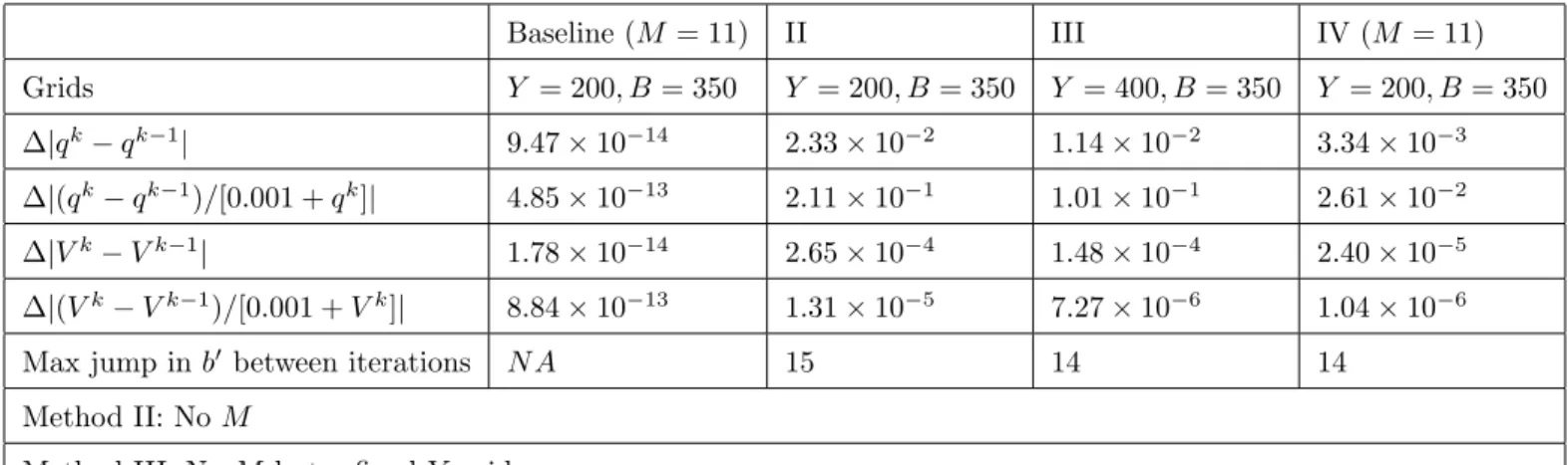
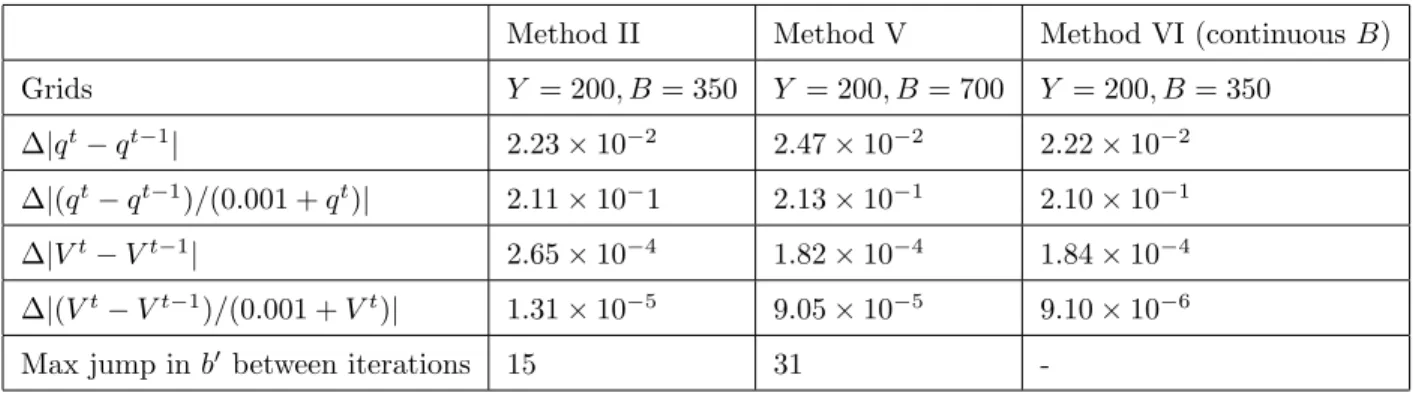
and the iteration is continued until max|H(qk, Zk) − qk| and max|Zk+1 −Zk| are both sufficiently close to zero.
For the iterations to converge, a solution to (6) must exist. But if both y and b are discrete and mis identically zero, there is no assurance that (6) will have a solution because
H(q) need not be continuous in q: For instance, for some q and (y, b,0), the sovereign will be indifferent between default and repayment and an infinitesimal change in q will cause a switch in behavior and, therefore, a discrete change in the expectation on the r.h.s. of (6). Similarly, even if the sovereign strictly prefers to repay, it may be indifferent between two different choices of debt. Once again, an infinitesimal change in q can result in a discrete change in behavior and a discrete change in the expectations term. Note that the scope for getting jumps due to indifference is much greater for long-term debt than short-term debt because of the fact that a(y, m,0) appears in the pricing equation.11 This additional
complication of long-term debt cannot be attenuated by making the grid on B fine because the points of indifference can be far apart on the grid. The budget set under repayment is typically not convex. Figure 1 shows a portion of q(y, b0)[b0−(1−λ)b] function for the case in whichb= 0 andm= 0 from our quantitative model presented later in the paper. Observe the kink and the ensuing depression in the upward sloping portion of the function. Figure 2 displays the variation in total lifetime utility from different choices ofb0 forb = 0 andm = 0. Observe the many nonconcave segments in this function. These nonconcavities imply that, given (y, b) and q, the sovereign may be indifferent between two widely separated values of
b0,which will make the r.h.s of (6) discontinuous in q.
In Appendix B we document that solving the model without the m shock leads to poor convergence outcomes for the equilibrium pricing function. The points markedA(the global maximum) and B (a local maximum) in Figure 2 illustrate what goes wrong. When the variance of m is set to 0, it often happens that a point like A is the optimal choice for some iteration k, but when that choice is incorporated in the price function, a point like B
11Exact indifference never happens in computations but changes inq from one iteration to the next are
not infinitesimal either. The point is that if two options are near-indifferent, very small changes inqk can
becomes the optimum choice for some iterationk0 > k; and when that choice is incorporated in the price function, the pointAre-emerges as the new optimum for some iterationk00 > k0. Thus, the asset decision rule meanders back and forth and (7) fails to converge. We suspect that this lack of convergence occurs because there is, in fact, no solution to (6).12
We know from general equilibrium theory that nonexistence resulting from nonconvexities can be avoided by allowing agents to randomize over decisions. Introducing m is like intro-ducing randomization: There is now a probability that an action dorb0 is chosen given (y,b) and q and this probability changes continuously withq. The nonconvexity of the budget set and nonconcavity of the value function continue to imply that the decision rulea(y, m, b;q) is a discontinuous function ofq. But as long as the points of discontinuity are finite in number, infinitesimal changes in q will not cause jumps in the expectation term (which is now an integral over y0 and the continuous variable m0) since each jump point has probability zero. In this way, a continuous CDF for m ensures the continuity of the r.h.s of the functional equation (6) with respect to q and the existence of an equilibrium.13
However, the introduction of m brings its own computational issues. Since m is a con-tinuous variable and non-convexities makea(y, m, b;qk, Zk) potentially discontinuous in m, it is not obvious how this potentially discontinuous decision rule is to be computed. This is where the assumption thatm is i.i.d. plays an important role – it allows us to establish that
d(y, m, b) anda(y, m, b) are monotone with respect tom, which, in turn, allows us to devise an algorithm to recover the decision rules near-exactly. We have:
12We consider an algorithm to have failed to converge if the maximum relative error between two successive
iterates of the price function does not fall below 10−5 within 3000 iterations. If the lack of convergence is
due to non-existence of an equilibrium then no matter how long we allow the program to run, it will not converge. Given this, some stopping rule is needed and we chose 3000 (we have confirmed that the algorithm without the iid shock does not converge for higher bounds as well).
13An alternative strategy to prove existence is to work with decision correspondences (as opposed to
decision rules). In this approach, if the decision-maker is indifferent between two (or more) actions then each action is taken with some probability that is determined in equilibrium. The proof of existence of an equilibrium relies on the Kakutani Fixed Point Theorem for compact and convex-valued correspondences. While this approach solves the existence issue, it does not appear to be computationally tractable. In particular, computing mixed strategies when the “support points” of the mixed strategy are not known in advance – and the choice set is very large – seems to be a challenging task.
Proposition 4: a(y, m, b) is increasing inm and d(y, m, b) is decreasing inm.
The task of computing the decision rules with respect tomthus boils down to (i) locating the value ofmat whichd(y, m, b;qk, Zk) switches from 1 to 0 and (ii) the values ofmat which the a(y, m, b;qk, Zk) switches from one debt level to a lower debt level.14 Note that it is not
known in advance which lower value of debt the sovereign switches to asmincreases because
a(y, m, b;qk, Zk) may be discontinuous in m and the lower debt level need not be the next lower debt level on the grid. However, an algorithm exists, described in Appendix B, that can check for these discontinuities and recover a(y, m, b;qk, Zk) correctly.15 Once behavior
with respect to m is known, max{Xk(y,−m¯), Vk(y, m, b;qk, Zk)} =Wk(y, m, b;qk, Zk) can be integrated with respect to m accurately using the integration method also described in Appendix B.
Another issue is that the iteration (7) may fail to converge if the variance of m is too small. As q changes, the thresholds for m change. If the variance of m is very small, any given change in thresholds will result in a large change in the choice probabilities. Setting
ζ very close to 1 can counteract this sensitivity (by making the change qk+1−qk itself very small) but at the expense of making the number of iterations needed to achieve convergence much larger than our upper bound of 3000. Thus, to achieve convergence σm must not be
14The behavior ofd(y, m, b) with respect tomis easy to characterize also because of the assumption that
the act of default resetsmto−m¯. This assumption makes the payoff from default independent ofm. If the level of transitory income were to remain unaffected by the act of default, the payoff from default,X, would also depend positively onm. As shown in Chatterjee et al. (2007), this would result in the default set being characterized bytwo thresholds,mL andmU, with default occurring whenm∈(mU, mL). Since the role of the transitory shock in this paper is to ensure convergence of (7), it is computationally efficient to eliminate the dependence ofX onmso that only one default threshold needs to be computed.
15For each (y, b) and q, the algorithm recovers {−m < m¯ K−1 < mK−2 < . . . < m1 < m¯} and {b0K < b0K−1 < . . . < b01} such thatb0K is chosen form∈[−m, m¯ K−1),b0K−1 is chosen form ∈[mK−1, mK−2), . . . ,b01is chosen form∈(m1,m¯] (K= 1 means the same debt levelb01is chosen for allm∈M). Note that K−ineed not be adjacent toK−(i+ 1) on the grid. Note also that it is not possible to apply these methods to a continuousy becauseyis not i.i.d and, therefore, the debt decision rule and the default decision rule are nonmonotonic iny. For instance, if currenty is above its mean, the price of debt is low, and the sovereign has an incentive to issue more debt. On the other hand, an above-meany implies that the country will be poorer in the future, which gives the sovereign an incentive to borrow less. These two effects pull in opposite directions and result in nonmonotonic behavior ofb0 with respect toy. In the absence of monotonicity, it is unclear if an algorithm can be devised to locate the values ofy at which there is a switch in debt levels or default decision.
too small.16 More generally, there is a tradeoff between σ
m and ζ with regard to achieving convergence: The lower is σm, the higher must ζ be to achieve convergence (an example of this tradeoff is given in the Web Appendix).
The final computational point is whether there are advantages to solving long-duration debt models assuming that y and b are discrete as opposed to continuous. We believe there are two advantages. First, if eitheryorb(or both) is a continuous variable,q(y, b0) is infinite-dimensional and it is much harder to establish the existence of a solution to q = H(q). If a solution is not guaranteed, and a computational algorithm fails to converge, it is not possible to tell if this failure results from a lack of a solution or from a defective algorithm. Second, with continuous y and/or b0, any computation scheme must involve interpolating value functions and the price function. For the interpolations to be justified, the functions must be smooth (i.e. differentiable) (see, for instance, Theorems 6.7.3 and 6.9.1 in Judd (1998)). But for this class of models neither value functions nor the price function are smooth everywhere.17
16Although we cannot prove that there is a unique equilibrium, we have not found instances of multiple
equilibria. We do know, theoretically, that given the price vectorq(y, b0), and a tie-breaking rule in case of indifference, the decision rulesd(y, m, b) anda(y, m, b) are unique (see the Web Appendix for a proof).
17How well interpolation techniques work in practice is an open research question. Hatchondo, Martinez
and Sapriza (2010) show that for the one-period debt model, interpolation techniques can deliver accurate results in the sense that interpolation methods give the same answer as the discrete state space method with a very fine grid for the model described in Arellano (2008). They apply a variant of their method to their long-duration bond model in Hatchondo and Martinez (2009) but they do not compare how well their method performs in solving the pricing equation relative to the discrete state space method. Also, it is not known if interpolation methods work well for the empirically relevant parameter space. In Arellano (2008), Hatchondo, Martinez and Sapriza (2010) as well as in Hatchondo and Martinez (2009), the level and volatility of spreads, as well as the level of debt, are quite low relative to the data.
5
Maturity, Indebtedness, and Spreads: The
Argen-tine Case
5.1
Calibration
We apply the framework developed in the previous sections to Argentina. The main con-tribution is to show that long-duration bonds, besides being a closer fit with reality, can help account for the average level of spreads, the volatility of spreads, and the average level of debt in Argentina without generating counterfactual implications regarding Argentina’s business cycle facts. Thus, introducing long-duration bonds into the Eaton-Gersovitz model significantly improves its quantitative performance. We focus on the 8-year period between 1993:Q1 and 2001:Q4 during which Argentina was on a fixed exchange rate vis-a-vis the dollar and was borrowing in international credit markets via marketable bonds.18
For the quantitative work we make the following specific functional form or distributional assumptions. • Endowment processes: lnyt =ρlnyt−1+t, where 0< ρ < 1 and t∼N 0, σ2 mt∼ trunc N 0, σm2
with points of truncation −m¯ and ¯m
• Utility function: u(c) =c1−γ/(1−γ).
• The loss in the persistent component of output in the event of default or exclusion:
φ(y) = max{0, d0y+d1y2}, d1 ≥0.
The specification for φ(y) allows for a variety of cost functions. If d0 >0 and d1 = 0, the
cost is proportional to output; if d0 = 0 andd1 >0,the cost rises more than proportionately
with output; if d0 < 0 and d1 > 0, the cost is 0 for 0 ≤ y ≤ −d0/d1 and rises more than
proportionately with output for y > −d0/d1. This last case resembles the cost function in
Arellano (2008).19 The reasons for choosing this flexible form are discussed in the findings
section.20 With these assumptions, the numerical specification of the model requires giving
values to 11 parameters. These are (i) three endowment process parameters, σm, ρ and
σ2; (ii) two preference parameters, β and γ; (iii) two parameters describing the bond, the maturity parameter λ, and the coupon payment z; (iv) two default output loss parameters,
d0 and d1, (v) the probability of re-entry following default, ξ; and (vi) the risk-free rate rf. The parameters of the endowment process are estimated on linearly detrended quarterly real GDP data for the period 1980:1-2001:4.21 As noted earlier, convergence of (7) requires
that the standard deviation of the i.i.d. shockmbe not too low. Experimentation shows that
σm = 0.003 is a good lower bound for our purposes – meaning that convergence is achieved within 3000 iterations for a wide range of parameter values. Thus, the endowment process is estimated assuming that σm = 0.003. The estimated value of ρ and σ are 0.948503 and 0.027092, respectively.22 In the computations, we approximate the y process by a 200-state
Markov chain and set ¯m = 2σm = 0.006.23 Of the preference parameters, the value of γ is set equal to 2, which is the standard value used in this literature.
19In Arellano, φ(y) = max{0, y−y¯}.Thus, cost is 0 for 0≤y ≤y¯and rises linearly at rate 1 beyond ¯y.
Thus, default costs as a proportion ofy,namely, (1−y/y¯ ),increase strongly withy.
20With this specification, the cost can exceedy for large y This situation never arises in our application
but could be formally ruled out by settingφ(y) = min{y,max{0, d0y+d1y2}}.
21The quarterly data series on real GDP, real aggregate consumer expenditure, real exports, real imports
and the (nominal) interest rate on Argentine sovereign debt is taken from Neumeyer and Perri (2005). All the quantity variables were deseasonalized using the multiplicative X-12 routine in EViews.
22If the process is estimated without the transitory shock, the estimates ofρandσ
are 0.930139 (0.038395)
and 0.027209 (0.001577), respectively, where the values in parenthesis are standard errors. Note that the values ofρand σ used in the calibration are well within 1 standard deviation of these AR1 estimates and
statistically indistinguishable from them. Note also that adding m to the AR1 equation is equivalent to assuming that log GDP is measured with some noise. Since the standard deviation of log GDP in the sample is 0.076107, setting σm = 0.003 implies that σm2 is 0.16 percent of the variance of log GDP. This is small
compared with the standard deviation of measurement errors assumed in estimation of DSGE models (see, for instance, Ireland (2004); see Del Negro and Schorfheide (2010, p. 53 ) for a discussion of this practice).
23The value of ¯mis small enough that the requirementy−max{0, d0y+d1y2} −m >¯ 0 is satisfied for all
The parameters describing the bond were determined to match the maturity and coupon information for Argentina reported in Broner, Lorenzoni, and Schmukler (2007). The median maturity of Argentine bonds is 20 quarters so λ = 1/20 = 0.05. We set z = 0.03, corre-sponding to an annual coupon rate of 12 percent. In the data, the value-weighted average coupon rate is about 11 percent.24
We setξ= 0.0385, which gives an average period of exclusion of 26 quarters, or 6.5 years. One measure of the exclusion period is the time it took to reach settlement on the defaulted debt. Beim and Calomiris (2000, Table A) report that for the 1982 Argentine default, settlement did not occur until 1993. For the 2001 default, Argentina reached settlement with a majority of its creditors in 2005. Benjamin and Wright (2009, Figure 15) also report Argentina as being in a state of default between 1982 and 1993 and between 2001 and 2005. By these measures, the average exclusion period for Argentina is 7.5 years. Gelos, Sahay and Sandleris (2008) measure exclusion as the years between default and the date of the next issuance of public and publicly guaranteed bonds or syndicated loans. By this measure, exclusion following the 1982 default lasted only 4 years (Table A7). They do not report the exclusion period for the 2001 default. In our calibration, we give somewhat more weight to the settlement-date measures of the exclusion period and set the average exclusion period to 6.5 years.
The risk-free rate, rf, was set at 0.01, which is roughly the real rate of return on a 3-month (one quarter) U.S. Treasury bill.
The three remaining parametersβ,d0, andd1are selected to match (i) an average external
debt-to-output ratio of 0.7, which is 70 percent of the average external debt-to-output ratio for Argentina over the period 1993Q1-2001:Q4; (ii) the average default spread over the same period of 0.0815; and (iii) the standard deviation of the spread of 0.0443.25 We seek to
24We chose 12 percent because with an annual risk-free rate of 4 percent and an average spread of around
8 percent, a bond with coupon of 12 percent will trade roughly at par. So, whether the debt is recorded at face value (which is the accounting practice) or at market prices (which is economically more sensible) will not matter for the calibration of the model.
25Debt is total long-term public and publicly guaranteed external debt outstanding and disbursed
match only a portion of debt because we do not model repayment. In reality, sovereign debt that goes into default eventually pays off something. In Argentina’s case, the repayment on debt defaulted on in 2001 has been around 30 cents to the dollar. Thus, we treat only 70 cents out of each dollar of debt as the truly unsecured portion of the debt. But, as part of our sensitivity analysis, we also examine the case in which we fully match average external debt-to-output ratio.
Finally, we need to specify the model analogs of the external debt-to-output ratio and spreads. In the GDF database, the external commitments of a country are reported on a cash-accounting basis, which means that commitments are recorded at their face value, i.e., they are recorded as the undiscounted sum of future promised payments of principal.26 The
coupon payments agreed to do not figure directly in this accounting because they are not viewed as obligations until they are past due. Given this valuation principle, the model analog of debt as reported in the data is simply b, and the external debt-to-output ratio is simply b/y.27 The default spread in the model is calculated as in the data. We compute
an internal rate of return r(y, b0)which makes the present discounted value of the promised sequence of future payments on a unit bond equal to the unit price, that is, q(y, b0) = [λ+ (1−λ)z]/[λ+r(y, b0)]. The difference between (1 +r(y, b0))4−1 and (1 +r
f)4 −1 is
the annualized default spread in the model.28
The parameter selections are summarized in the following two tables. Table 1 lists the
Global Development Finance Database (series DT.DOD.DPPG.CD). The average debt-to-output ratio is the average ratio of debt to GNP measured at a quarterly rate. The spread was calculated as the difference between the interest rate data reported in Neumeyer and Perri (which is the same as the EMBI data) and the 3-month T-bill rate. The T-bill rate series used is the TB3MS series available at
http://research.stlouisfed.org/fred2/categories/116. Both the interest rate data and the T-bill rate are reported in annualized terms.
26See “Coverage and Accounting Rules” in Section 3 of the World Bank Statistical Manual on External
Debt (also available at http://go.worldbank.org/6FB4093970).
27The reason for this is that each bond can be viewed as a combination of unit bonds with varying
maturities. For instance, a measureλof unit bonds is due next period, a measure (1−λ)λis due in 2 periods, . . . , a measure (1−λ)j−1λis due inj periods, and so on. Since each of these obligations has a face value of
1, each would be recorded as a unit obligation. Thus, the total obligation is simplyP
j=1λ(1−λ)
j−1= 1.
28If there is no possibility of default, the unit price would be a constant ¯qsuch that ¯q= [λ+ (1−λ)(z+
¯
q)]/[1 +rf],which implies ¯q = [λ+ (1−λ)z]/[λ+rf]. Since q(y, b) ≤ q,¯ it follows that r(y, b0) ≥ rf.
values of the parameters that are selected directly without solving for the equilibrium of the model. Table 2 lists the parameter values that are selected by solving the equilibrium of the model and choosing the parameters so as to make the model moments come as close as possible to the three data moments mentioned above.
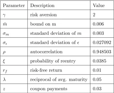
Table 1: Parameters Selected Directly
Parameter Description Value
γ risk aversion 2 ¯ m bound on m 0.006 σm standard deviation ofm 0.003 σ standard deviation of 0.027092 ρ autocorrelation 0.948503 ξ probability of reentry 0.0385 rf risk-free return 0.01 λ reciprocal of avg. maturity 0.05
z coupon payments 0.03
Table 2: Parameters Selected by Match-ing Moments
Parameter Description Value
β discount factor 0.95402
d0 default cost parameter −0.18819
d1 default cost parameter 0.24558
5.2
Findings
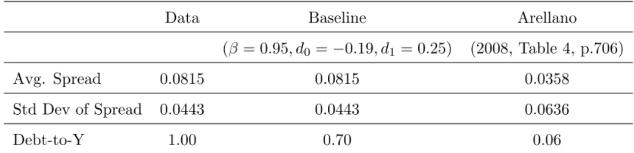
The results of the moment matching exercise are reported in Table 3. The first column of numbers shows the data for Argentina. The second column reports the moments in the model. All model moments are (sample) averages calculated by simulating the economy
over many periods but always discarding the first 20 periods after re-entry following each default.29 Evidently, the matching exercise is fully successful.30 Figure 3 shows the path
of the model-simulated spreads for 1993-2001 if the initial level of debt is chosen to exactly match the spread in 1993:Q1. The close correspondence between the model-implied spreads and the data is striking.
For comparison purposes, the last column reports the corresponding model statistics of Arellano’s one-quarter debt model. Although Arellano did not target these statistics, the fact remains that there are significant deviations between her model and the data: The debt-to-output ratio is very low, the average spread is about 50 percent lower and the volatility of spreads is about 44 percent higher.
Table 3: Results and Comparison
Data Baseline Arellano (β = 0.95, d0 =−0.19, d1= 0.25) (2008, Table 4, p.706) Avg. Spread 0.0815 0.0815 0.0358
Std Dev of Spread 0.0443 0.0443 0.0636 Debt-to-Y 1.00 0.70 0.06
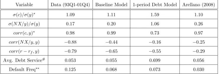
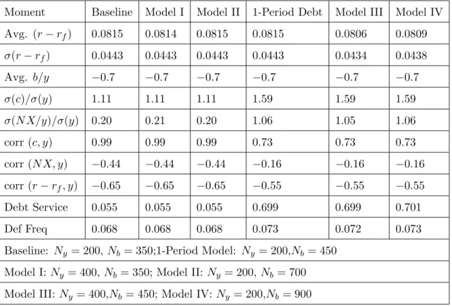
Table 4 reports some key cyclical properties of Argentine data and corresponding model moments.31 Since we did not target these moments, the results are informative about the performance of our model.
29We do this because the model economy re-enters capital markets without any debt, whereas Argentina
emerged from each default/restructuring episode with debt. By ignoring the first five years following re-entry, we ignore years with counterfactually low debt in our model.
30For the record, the average debt-to-output ratio in the baseline model when debt is measured at its market
value is 0.703. So, it is only slightly higher than its face value. The reason is that the average interest rate on debt, 0.0292 percent per quarter, is only slightly larger than the 0.0285 (= (1−λ)z= 0.95×0.03)) coupon payment on each unit of debt.
31Second moments for consumption and output were computed using logged and linearly de-trended series.
Since net exports (NX) can be negative, it was expressed as a proportion of output and then linearly de-trended. The spread series was also linearly detrended, although the trend component is negligible.
Table 4: Cyclical Properties, Data and Models
Variable Data (93Q1-01Q4) Baseline Model 1-period Debt Model Arellano (2008)
σ(c)/σ(y)∗ 1.09 1.11 1.59 1.10
σ(N X/y)/σ(y) 0.17 0.20 1.06 0.26
corr(c, y)∗ 0.98 0.99 0.73 0.97
corr(N X/y, y) −0.88 −0.44 −0.16 −0.25
corr(r−rf, y) −0.79 −0.65 −0.55 −0.29
Avg. Debt Service# 0.053 0.055 0.699 0.056 Default Freq∗∗ 0.125 0.068 0.073 0.030 ∗Sample period: 1980:Q1-2001:Q4;∗∗Sample period:1975-2001
# Principal and interest payments as a fraction of output
The first column of numbers is the data for Argentina. Several features of the data stand out. First, the relative volatility of consumption is about the same as output – in stark contrast to small, open, developed economies. Second, the trade balance is countercyclical, which is also in contrast to small, open, developed economies. Third, spreads on sovereign debt are countercyclical and Argentina displayed a high propensity to default during the 1975-2001 period.32 The following column reports the same statistics for the model. The
model gets the qualitative patterns of the data right: Model consumption and trade balance have about the right level of volatility relative to output, and the trade balance and spreads are countercyclical while consumption is highly procyclical. The forces in the model that lead to these patterns are the ones emphasized in Aguiar and Gopinath (2006) and Arellano (2008).33 The average probability of default in the model is lower than the observed frequency
32The frequency of default is the number of default episodes as a fraction of the number of years Argentina
was in good standing with international creditors in the 27 years between 1975-2001. Argentina defaulted in August 1982 and re-gained access in March 1993. We assume that Argentina was in default for 11 years. Thus it defaulted twice in a 16-year period of good standing. We chose 1975 as the start date because that is when Argentina began accumulating significant amounts of debt. If we start in 1946 and use the “years in restructuring” reported in Beim and Calomiris (2000, Table A), Argentina would show three defaults in a 35-year period of good standing. This would give a default frequency of 0.086. If we start in 1800 and use Beim and Calomiris again, the default frequency would drop to 0.03. But it is questionable if our model is the right framework to address such a long sweep of history.
of default; but default is a rare event and it is hard to estimate its frequency accurately from relatively short data series.
The second column reports results if debt is assumed to be one period and (β, d0, d1) are
chosen to match the same three statistics as in the baseline model. The parameter vector that achieves this match is (0.67,−0.46,0.57). Aside from the implausibility of such a low value of β, the match generates serious anomalies with respect to business cycle statistics. The relative volatility of consumption and the trade balance is now much higher than in the data and the correlations of consumption, the trade balance and spreads with output are much lower. Incorporating long-term debt moves virtually every model moment in Table 4 closer to the data, a clear indicator of the superior performance of the long-term debt model. Why does the one-period debt model imply such a high volatility of consumption? The reason is simple: If there are b dollars of debt outstanding, the debt service obligation is
b and the sovereign must refinance all of b at the new price q(y, b) to maintain its debt level. Thus, changes inq(y, b) will tend to imply large changes in consumption and the trade balance because b is large relative to output. In contrast, with long-term debt, the debt service obligation is only [λ+ (1−λ)z]b and the sovereign can maintain its debt level by refinancing the much smaller quantityλbat the new priceq(y, b). Thus, for a given volatility of spreads, the long-term debt model can match the average level of debt without creating a counterfactually high volatility of consumption and the trade balance.
The last column reports the results for the benchmark model in Arellano (2008, Table 4). Even ignoring the frequency of default, the model with long-term debt comes substantially closer to accounting for the cyclical moments. In Arellano’s model, the (negative) correlations between net exports and output and spreads and output are, on average, about 33 percent as large as in the data. In contrast, in the model with long-term debt these correlations, respectively, are 50 percent and 82 percent as large as in the data.
it is optimal for the sovereign to reduce debt rather than to increase it (which is what would be optimal holding interest rates constant). Thus, there is a tendency for consumption to decline more than the decline in output and for the trade balance to improve with a fall in output.
5.3
Model Mechanics
5.3.1 Role of the Default Cost Function
Since the calibrated valuesd0 andd1 are negative and positive, respectively, our specification
shares the feature that Arellano introduced in her specification of default costs, namely, that the default cost as a proportion of output declines with output and becomes zero for low enough output levels.
It is now well-understood that this structure of default punishment is important in gen-erating higher default rates, whether the default cost function is endogenous or exogenous (see, for instance, the discussion in Mendoza and Yue (2009)). The key is the asymmetry in default costs: The country is punished much more severely for default when income is high than when income is low. The severe punishment for default in high-income periods implies that investors do not expect the sovereign to default in the near future (given the persistence in output). This results in low spreads, and the (impatient) sovereign borrows aggressively. But when output declines, the punishment from default declines as well. This raises the likelihood of default and spreads rise. The high spreads make debt servicing more onerous, and, eventually, if income stays low, the sovereign defaults. Without the asymme-try, it is impossible to generate a significantly positive default frequency without making the sovereign very impatient.34
What appears not to have been appreciated in the literature is that the structure of default costs is also important for the volatility of spreads. For Arellano’s specification, the default cost as a proportion of output is 1−y¯· y−1 (where ¯y is the level of output
below which costs are zero), which is very sensitive to changes in y. Consequently, the probability of default is correspondingly sensitive to fluctuations in y and so is the spread (recall that Arellano’s model predicted a higher volatility of spread than the data). With
34For instance, with a proportional default cost, the cost does not vary much with the level of output
and spreads remain relatively high over a wide range of output and debt levels. Consequently, the sovereign rarely borrows enough to enter into regions where the probability of default is measurably positive (unless the sovereign is very impatient).
our specification, we can match both the level and the volatility of spreads. The larger d1
is, the more volatile the spreads are likely to be. This intuition is verified in Table 5 which shows the results of varying d1 while choosing d0 and β to match the targets for average
debt-to-output ratio and the average spreads. Notice that the volatility of spreads rises with
d1.
Table 5: Role of Default Cost Parameters
d1 d0 β σ(r−rf) avg. (r−rf) avg. b/y
0.15 −0.098 0.93696 0.0264 0.0815 0.70 0.25 (baseline) −0.188 0.95402 0.0443 0.0815 0.70 0.35 −0.288 0.96195 0.0577 0.0815 0.70
The accompanying changes inβandd0 are informative about the economics of the model
and are worth commenting on. The higher is d1 the more sensitive spreads are to variation
in output and the easier it is for the model to achieve a higher frequency of default. Since higher default frequency and high spreads are easier to achieve with a higherd1, the sovereign
needs to be more patient in order for it to willingly hold the level of debt that implies the observed probability of default. This explains why the value of β rises with d1. We also see
that d0 falls as d1 rises. This is because an increase in d1 shifts up the default cost function
which expands the maximum amount of debt the sovereign can carry without defaulting. As long as β is sufficiently less than 1/(1 +rf), the sovereign will gravitate to this maximum and that will increase the average level of debt. To keep the average debt level constant, the overall default punishment should remain roughly constant. Thus, d0 falls to counterbalance
the increase in d1.
5.3.2 The Role of Long-term Debt
In this section, we explain the role of long-term debt in our model. One way to understand its role is to compute the equilibrium of the baseline model with short-term debt, i.e., all
parameter values are held fixed at their baseline values but the sovereign is permitted to issue only one-period debt. The results of this exercise are shown in the last column in Table 6. The equilibrium has stark differences. The average spread, the volatility of spreads, and the default frequency are minuscule compared with the long-term bond case.
Table 6: Role of Long-term Debt
Moment Data Baseline Baseline Model w/ λ= 1 Avg. (r−rf) 0.0815 0.0815 0.0026 σ(r−rf) 0.0443 0.0443 0.0037 Avg. b/y 1 0.70 0.81 σ(c)/σ(y) 1.09 1.11 1.14 σ(N X/y)/σ(y) 0.17 0.20 0.34 corr(c, y) 0.98 0.99 0.95 corr(N X/y, y) −0.88 −0.44 −0.24 corr(r−rf, y) −0.79 −0.65 −0.42 Debt Service 0.053 0.055 0.812 Def Freq 0.075 0.068 0.002
This raises the question as to why increasing the maturity length beyond one period in-duces the sovereign to willingly extends its borrowing into the region where the probability of default is significantly positive. The answer lies in the differing incentives to issue additional debt in the two cases. Treatingb0 as a continuous variable, the marginal gain from borrowing is given by: −q(y, b0)− ∂q(y, b 0) ∂b0 [b 0 − (1−λ)b] u0(y+m+ [λ+ (1−λ)z]b−q(y, b0) [b0−(1−λ)b]) (9)
When the sovereign issues an extra unit of debt, it gets revenue from that extra unit but faces a decrease in the price of the bond, which decreases the revenue on all bonds being
currently issued. In the case of short-term debt, the decrease in price applies to the entire stock of debtb0, whereas with long-term debt it applies to [b0−(1−λ)b].Thus, the sovereign faces a much greater disincentive to borrow when default probabilities become positive in the short-term case.
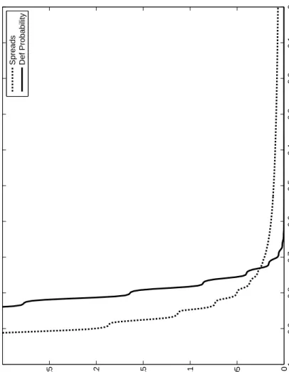
In addition, |∂q(y, b0)/∂b0|is larger for short-term debt in the region where default prob-abilities are positive, as shown in Figures 4 and 5, which plot how spreads and the default probability vary with debt in the two cases. The reason why spreads rise faster with short-term debt is that servicing one-period debt becomes onerous more quickly than servicing long-term debt. Although debt levels are not perfectly comparable across the two cases (they involve different future obligations), the fact that spreads rise faster for short-term bonds is another reason the sovereign is less willing to extend borrowing into the region where default probability is positive when debt is short-term.35
5.4
The Welfare Cost of Debt Dilution
In this section, we examine the welfare effects in the baseline model of moving from one-period debt (λ= 1) to long-term debt (λ= 0.05). We assume that thebandmare both zero and compute ΣyVλ(y,0,0)Π(y),where Π(y) is the invariant distribution of the Markov chain fory. Rather than report utilities, we report the value ofcthat makesc1−σ/[(1−β)(1−σ)] equal to ΣyVλ(y,0,0)Π(y) (the flow certainty equivalent consumption). The results are given in Table 7.
35It is worth noting that spreads on long-term debt start out positive and rise even though the probability
of default next period may be zero. Even when the sovereign borrows a very small amount in the current period (so the default probability for next period is 0), lenders understand that the sovereign’s optimal decisionnext period is to take on a significant amount of debt. And sinceq(y, b0) is decreasing inb0,lenders rationally expect to suffer a capital loss on the nonmaturing portion of the debt. This depresses the current price of debt and leads to a positive spread from the start. And, initially, the spread rises with debt simply because thea(y0, m0, b0) is increasing inb0 (Proposition 3), and the expected capital loss is increasing. This shows that it is not necessary to invoke risk-aversion on the part of lenders to account for gaps between spreads and default probabilities. With long-term debt, a gap can arise (and vary) because of the dynamics of debt accumulation. A gap can also arise if there is repayment on defaulted debt, which we have ruled out.
Table 7: Welfare Comparison Across Maturity Length
(Quarters, λ) Cert. Eqv. Cons Avg. Spread Avg. b/y Def Freq (1,1) 1.0175 0.0026 0.81 0.0024 (2,0.5) 1.0174 0.0049 0.81 0.0047 (4,0.25) 1.0169 0.0102 0.79 0.0096 (6,0.167) 1.0161 0.0166 0.76 0.0156 (8,0.125) 1.0150 0.0241 0.74 0.0224 (10,0.1) 1.0139 0.0327 0.73 0.0298 (12,0.083) 1.0129 0.0420 0.71 0.0375 (14,0.071) 1.0118 0.0519 0.70 0.0455 (16,0.063) 1.0108 0.0619 0.70 0.0534 (18,0.056) 1.0099 0.0719 0.70 0.0608 (20,0.05) 1.0092 0.0815 0.70 0.0675
Welfare is highest for short-term debt and declines monotonically as λ falls toward 0.05. Thus, the sovereign is best off issuing short-term (one-quarter) debt. The difference in consumption equivalent in going from 20-quarter maturity to 1-quarter maturity is 0.81 percent, which is significant by the standards of welfare comparisons.
Why is short-term debt better than long-term debt? If the sovereign can commit to not default, the (implicit) interest rate on short-term and long-term debt would be the risk-free rate and maturity length would make no difference to welfare or consumption. Evidently, the risk of default makes a difference. But the reason for the difference is subtle. It turns out that if lenders insist that the sovereign compensate them for declines in the market value of outstanding debt and, conversely, the sovereign insists that the lenders compensate the sovereign for improvements in the value of outstanding debt, long-term debt becomes equivalent to short-term debteven in the presence of the default risk. This equivalence result is formally demonstrated in Appendix C. Thus, freezing the value of future outstanding debt at its current market value makes long-term and short-term debt equivalent.
If the future value of outstanding debt is fixed at its value at issue, the sovereign cannot dilute the future value of outstanding debt by issuing more debt in the future. This arrange-ment, therefore, solves the debt dilution problem and reduces the interest rate on debt. On the other hand, the future market value of debt can also change due to changes in y and these exogenous fluctuations in the market value of outstanding debt lead to corresponding fluctuations in disposable income of the risk-averse sovereign.36 For our calibration, the
reducing effect of a more volatile disposable income is dominated by the welfare-enhancing effect of lower borrowing costs, making short-term debt better than long-term debt.37
5.5
Rollover Crises and the Superiority of Long-Term Debt
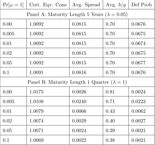
The results of the previous section lead to the awkward conclusion that even though long-term debt improves model performance, in the model itself the sovereign would prefer to issue one-period debt. In this section we extend the baseline model to allow for a small probability of a rollover crisis (self-fullfilling default) and show that this small additional source of shocks makes long-term debt better than short-term debt without affecting the superior performance of the long-term debt model emphasized earlier.
This extension is motivated by the following two observations. First, if the sovereign issues short-term debt in our model, it issues a large amount of it – on average 81 percent of mean output. Thus, the sovereign rolls over a very large fraction of current consumption each period, on average. Second, many observers have noted that a large volume of short-term debt exposes a borrower to the possibility of a “run equilibrium” wherein lenders’ refusal to roll over maturing debt can force the borrower into default, thereby justifying the lenders’
36When the market value falls, the sovereign makes a payment to lenders and when the market value rises
the sovereign receives a payment from lenders.
37In an earlier version of the paper, we showed that if we give the sovereign a choice between
short-term and long-short-term debt each period, and we match the same three statistics as in the baseline model, the sovereign always chooses to issue short-term debt in every state. These results are available in the working paper version of this paper. Note, however, that to solve this model in reasonable time we employed a much coarser grid forY andb than in the baseline model.
refusal to lend. Cole and Kehoe (2000) provide a theoretical foundation for this view in the context of sovereign borrowing. Importantly for our purposes, they also show that the “run equilibrium” is less likely if the sovereign issues long-term debt. Even with a large stock of long-term debt, the maturing portion of debt can be small, so lenders’ refusal to roll over is of little consequence to the borrower. Knowing this, lenders do not run and runs fail to be an equilibrium outcome.
Cole and Kehoe assumed that the level of debt is given. In our model, the sovereign gets to choose the level of debt. As in Cole and Kehoe, it is also the case for us that the probability of rollover crisis is higher for short-term debt when the level of debt is high. But, given the higher probability of a crisis, the sovereign chooses to borrow less when debt is short term and, in equilibrium, the probability of rollover crises is low for short-term debt also. But the reduction in borrowing leads to a reduction in welfare relative to long-term debt.
To proceed, consider the following static coordination game played by the sovereign and a single new lender at the start of any period in which the sovereign has some outstanding debt and, conditional on meeting its current obligations, desires to issue new loans. The columns give the strategies of the sovereign and the rows give the strategies of the lender. If the lender makes the new loan (L) and the sovereign repays its existing debt (R), the sovereign receives the payoff from repaying the loan and borrowing, denoted V+(y, m, b), and the lender earns
a net return of 0 (i.e, the lender earns the risk-free return – in expectation – which is also the opportunity cost of its funds). If the lender lends and the sovereign defaults (D), we assume that the new loan is returned to the lender without it earning any interest – hence the (discounted) loss of interest earnings (rf/(1 +rf))∆, where ∆ is the amount of new lending.38 If the lender does not lend (N) and the sovereign repays but cannot borrow, the sovereign receives V−(y, m, b) ≤ V+(y, m, b) and the lender earns 0. Finally, if the lender
38In Cole and Kehoe, the game is sequential with the sovereign deciding on default after lenders have made
their lending decisions. If we had followed Cole and Kehoe, the payoff from default conditional on having received new loans would take into account the additional consumption afforded by the new loan. And, if lenders lend and the sovereign defaults lenders would lose not only the interest but the entire loan as well.
does not lend and the sovereign defaults, the payoffs are 0 andX(y,−m¯) for the lender and sovereign, respectively. R D L 0, V+(y, m, b) −(r f/1 +rf)∆, X(y,−m¯) N 0, V−(y, m, b) 0, X(y,−m¯) .
Under the tie-breaking rule that if the sovereign is indifferent between repaying and defaulting it always repays and if the lender is indifferent between lending and not lending it always lends, this game has the following set of Nash equilibria, depending on the value of
X(y,−m¯). When X(y,−m¯) ≤ V−(y, m, b) ≤ V+(y, m, b), the unique equilibrium is (L, R).
Similarly, if V−(y, m, b) ≤ V+(y, m, b) < X(y,−m¯), the unique equilibrium is (N, D). But
when V−(y, m, b) < X(y,−m) ≤ V+(y, m, b), both (L, R) and (N, D) are equilibria of the
game. In this case, we assume that the equilibrium selected depends on the realization of a sunspot variable, denoted ω : If ω = 0, the (L, R) equilibrium is selected and if ω = 1,
the (N, D) equilibrium is selected. The latter case corresponds to a self-fulfilling “rollover crisis”: The lender refuses to lend because it believes that the sovereign will default and the sovereign defaults because it believes that the lender will refuse to lend.39
In what follows, we modify the model presented in earlier sections in light of this game. First, we need to be precise about the valuesV+(y, m, b) andV−(y, m, b) andX(y,−m¯).Let
W(y, m, b, ω) denote the lifetime utility of the sovereign, which now depends on the sunspot variable ω in addition to the other state variables. Then,
V+(y, m, b) = max
b0∈B u(c) +βE(y
0m0)|y[(1−π)W(y0, m0, b0,0) +πW(y0, m0, b0,1)]
s.t. (10)
c=y+m+ [λ+ (1−λ)z]b−q(y, b0) [b0−(1−λ)b],
39In Cole and Kehoe, the game is played between the sovereign and many lenders acting independently.
The multiplicity of lenders makes the coordination failure implicit in a rollover crisis more plausible. For simplicity, we assume that a coordination failure may occur between the sovereign and a single lender.
where we assume thatω is i.i.d and takes the value 1 with probability π. If there is nob0 for which consumption is non-negative, then we set V+(y, m, b) to −∞. And
V−(y, m, b) = max b0∈B u(c) +βE(y 0m0)|y[(1−π)W(y0, m0, b0,0) +πW(y0, m0, b0,1)] s.t. (11) c=y+m+ [λ+ (1−λ)z]b−q(y, b0) [b0−(1−λ)b] b0 ≥(1−λ)b.
Again, if there is no b0 for which consumption is non-negative, we set V−(y, m, b) to −∞. Evidently, V−(y, m, b)≤V+(y, m, b). If the sovereign desires to issue new loans (conditional
on meeting its current obligations), V−(y, m, b) < V+(y, m, b). The value under exclusion has the same structure as in the rest of the paper, specifically, X(y, m) solves X(y, m) =
u(y−φ(y) +m) +β{[1−ξ]E(y0m0ω0)|yX(y0, m0) +ξE(y0m0ω0)|yW(y0, m0,0, ω0)}which then pins
down the value under default, X(y,−m¯).
The functional equation that determines W(y, m, b, ω) is given by
W(y, m, b, ω) (12) = V+(y, m, b) if X(y,−m¯)≤V−(y, m, b) and ω ∈ {0,1} X(y,−m¯) if V+(y, m, b)< X(y,−m¯) and ω∈ {0,1} V+(y, m, b) if V−(y, m, b)< X(y,−m¯)≤V+(y, m, b) andω = 0 X(y,−m¯) if V−(y, m, b)< X(y,−m¯)≤V+(y, m, b) andω = 1
To see why (12) holds, observe that when X(y,−m¯) ≤ V−(y, m, b) the unique equilibrium of the game is (L, R). Therefore, regardless of the value of ω, the (equilibrium) lifetime utility of the sovereign is V+(y, m, b). Similarly, when V+(y, m, b)< X(y,−m¯), the unique
equilibrium of the game is (N, D) and the lifetime utility of the sovereign is X(y,−m¯), regardless of the value of ω. When V−(y, m, b) < X(y,−m¯) ≤ V+(y, m, b), the equilibrium