University of Cape Town
for chlorophyll algorithm application
across multiple optical water types
in South African coastal waters
Marié Smith
Thesis presented for the degree of
Doctor of Philosophy
Oceanography Department
University of Cape Town
August 2016
quotation from it or information derived from it is to be
published without full acknowledgement of the source.
The thesis is to be used for private study or
non-commercial research purposes only.
Published by the University of Cape Town (UCT) in terms
of the non-exclusive license granted to UCT by the author.
The present work has been originally written by me, with the full support of my super-visors: Dr Marcello Vichi of the Department of Oceanography, University of Cape Town, South Africa; Dr Stewart Bernard of the Council for Scientific and Industrial Research, South Africa; Dr Mark Matthews of CyanoLakes (Pty) Ltd, Cape Town, South Africa. In addition, important contributions to the approach used in this study are clearly acknow-ledged through referencing within the text.
Ocean colour remote sensing is a valuable tool for deriving information about key biogeo-chemical variables over inland, coastal and ocean waters at scales unachievable viain situ
techniques. However, broader use of ocean colour data is still limited by the need for users to choose among a seemingly complicated range of available satellite products and to un-derstand the limitations and constraints of these products across a wide range of water types. This issue could benefit from the capability to seamlessly apply and blend water-type appropriate algorithms into a single output product that provides optimal retrievals over a wide range of water types. The assessment of the fuzzy membership of satellite re-mote sensing reflectance (Rrs) to pre-defined regional optical water types (OWTs) provides
a framework for application and blending of OWT-appropriate algorithms on a per-pixel basis. This study presents the first characterization of the OWTs in the coastal waters of South Africa. The OWTs are determined through stepwise fuzzy c-means clustering of a systematically expanding and modified database constructed from in situ, synthetic and
regionally extracted Medium Resolution Imaging Spectrometer (MERIS) Rrs. A
data-base division allows separate and more detailed clustering of phytoplankton-dominated Rrs and backscattering-dominated Rrs into six and five classes respectively. Chlorophyll
a (Chl a) algorithms are assigned per OWT based on lowest error and uncertainty. The
blended Chl a product consists of weighted retrievals from five different algorithms,
in-cluding two 4th order polynomial exponential algorithms utilizing the blue-green spectral
region, two red-NIR band ratio algorithms, and a neural network. The algorithm blending procedure retrieves satellite-derived Chl a concentration ([Chl a]) with lower RMS error
and uncertainty compared to individual algorithms and provides improved capability to retrieve [Chla] for different South African water types with a single product over a range
spanning almost four orders of magnitude. The eleven OWTs are utilized in the clas-sification and algorithm blending framework and applied to the full archive of MERIS Level 2 reflectance between the years 2002 and 2012 over South Africa’s coastal waters. The persistence of the OWTs is presented and linked to the prominent environmental and physical drivers, whilst regions with low total class membership sums are discussed
in terms of satellite data coverage and data quality. A time series of the blended [Chl
a] product displays improved capability to capture the ranges of variability observed in
the coastal, shelf and offshore environment compared to currently available regional and standard MERIS Level 2 products.
For providing funding and data, I would like to thank the following:
ACCESS for three and a half years of funding, covering my living costs, fieldwork and enabling me to attend numerous conferences. ESA for providing the satellite data needed for the project. ACRI-ST, ARGANS and ESA for access to the MERMAID system, and the following individual contributions to these data: Vanda Brotas and Carolina Sà for PortCoast data; David McKee for BristolIrishSea data; David Antoine for BOUSSOLE data; Sélima Mustapha and Simon Belanger for CASES data; Catherine Belin for Ifremer-REPHY data; David Siegel for PlumesAndBlooms data; Antonio Mannino, Frank Muller-Karger, Rick Gould, Kendall Carder, Greg Mitchell, David Siegel for NOMAD data; Guiseppe Zibordi, Jean-francois Berthon, and Elisabetta Canuti for BioOptEuroFleets data; Hubert Loisel for EastEngChannel and FrenchGuiana data. CSIR and DAFF for additional funding, equipment and research expertise needed for fieldwork.
For everything else, I would like to thank the following individuals:
Stewart Bernard for project supervision, advice, financial support, endless input on chapters, and keeping me relatively sane. Marcello Vichi and Mark Matthews for provid-ing valuable input and feedback on my chapters. Hayley Evers-Kprovid-ing and Lisl Robertson-Lain for limitless technical support and being my sounding board. Andy Rabagliati, Ray-mond Roman and Luke Gregor for technical support and assistance with data processing. My fellow PhD students Ffion Atkins, Lauren Biermann, Emma Bone and Christo Whittle for sharing and empathizing with my frustrations. I would like to thank my parents for inspiring my love for science and the ocean, and for continued emotional and financial support throughout my graduate and post-graduate career, enabling me to focus solely on my work. For all the laughs, wine, surf sessions and electronic rants, I want to thank my two best friends Karien Brand and William Dowd. Final thanks goes to my partner Rod Smith, who has provided me with all the love, support, and ice cream that a girl could ever need to get through this PhD!
a Total absorption coefficient (m−1)
aφ Phytoplankton absorption coefficient (m−1)
adg Combined CDOM and detritus absorption coefficient (m−1)
ag Absorption coefficient of CDOM (m−1)
aN AP Absorption coefficient of non-algal particulate matter (m−1)
aw Absorption coefficient of seawater (m−1)
A Average total class membership (per image)
AOPs Apparent optical properties
bbφ Phytoplankton backscattering coefficient (m−1)
bbφ/bφ Phytoplankton backscatter fraction
bbs Non-algal particulate backscattering coefficient (m−1)
[Chl a] Chlorophylla concentration (mg m−3)
CDOM Coloured dissolved organic matter
CE Classification entropy
CZCS Coastal zone color scanner
Ed Downwelling irradiance (µW cm−2 nm−1)
EAP Equivalent algal population
EOF Empirical orthogonal function
FCM Fuzzy c-means
fi Membership function
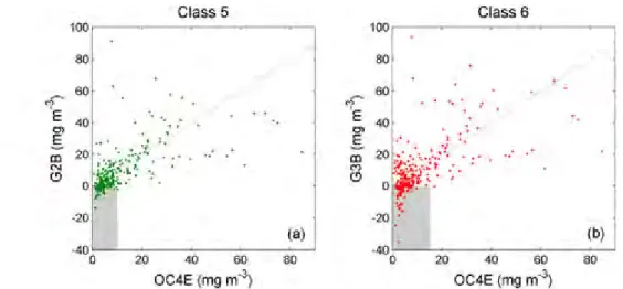
G2B Gilerson et al. (2010) 2-band algorithm G3B Gilerson et al. (2010) 3-band algorithm
TSRB Satlantic hyperspectral tethered surface radiometer buoy
IOPs Inherent optical properties
IOCCG International ocean colour coordinating group
IR Infrared
Lu Upwelling radiance (µW cm−2 nm−1 sr−1)
Lw Water-leaving radiance (µW cm−2 nm−1 sr−1)
KZN KwaZulu-Natal
MARE Median absolute relative error
MERCI MERIS catalogue and inventory
MERIS Medium resolution imaging spectrometer
MERMAID MERIS matchup in-situ database
MODIS Moderate resolution imaging spectroradiometer
MPH Maximum peak-height
NAP Non-algal particulate matter
NIR Near infrared
NOMAD NASA bio-optical marine algorithm dataset
OC3E 3-band algorithm developed for MODIS (O’Reilly et al.,1998), with coefficients derived for MERIS wavelengths
OC4E 4-band algorithm developed for SeaWiFS (O’Reilly et al., 1998),
with coefficients derived for MERIS wavelengths
OCMe MERIS algal pigment index for Case 1 waters algorithm (Morel and
Antoine, 2011)
OLCI Ocean and land colour instrument
OWTs Optical water types
P C Partition coefficient
PCA Principal component analysis
PCD1_13 Quality flag for the 13 MERIS reflectance bands
RMSE Root-mean-square error
Rn Integral-normalized Rrs
RR Reduced resolution
Rrs Remote sensing reflectance (sr−1)
ρw Water-leaving reflectance
S Separation index
SC Partition index
SeaWiFS Sea-viewing wide field-of-view sensor
TOA Top of atmosphere
z Depth (m)
Z2
Abstract iii Acknowledgements v List of notation vi Contents x 1 Introduction 1 1.1 General introduction . . . 1
1.1.1 The marine light field and the role of inherent optical properties . . 2
1.1.2 Chlorophyll a algorithms . . . 4
1.1.3 South African coastal waters: an ideal case for optical water type classification . . . 7
1.2 Objectives and key questions . . . 8
1.3 Thesis structure . . . 9
2 Data description, techniques and methodology 10 2.1 Introduction . . . 10
2.1.1 The history of data clustering and classification . . . 10
2.2 Chapter aims . . . 15
2.3 Data and methods . . . 16
2.3.1 Data description . . . 16
2.3.2 Data clustering and classification . . . 21
2.3.3 EOF analysis of cluster datasets and optical water type classes . . . 29
2.3.4 Class-specific Chla algorithms . . . 30
2.4 Synopsis . . . 35
3 Clustering results and Chlorophyll a algorithm selection 36 3.1 Introduction and chapter layout . . . 36
3.2 Results . . . 38
3.2.1 Dataset construction and cluster selection process . . . 38
3.2.2 Analysis of the optical variability within the clustering datasets . . 51
3.2.3 The optical water type classes: data composition and assessment of class overlap . . . 56
3.2.4 The optical water type classes: analysis of causal bio-optical vari-ability . . . 59
3.2.5 Descriptive qualities of the optical water type classes . . . 65
3.2.6 Class-specific Chla algorithm selection . . . 69
3.2.7 Validation of blended Chl a algorithm performance using matchup MERIS data . . . 79
3.2.8 The potential for weighted uncertainty maps for blended Chloro-phyll products . . . 82
3.3 Discussion of results . . . 84
3.3.1 Relevance and soundness of clustering and classification methods driven by application . . . 84
3.3.2 The building blocks of a clustering database: the effects of database composition . . . 86
3.3.3 Transferability of the methods . . . 94
3.3.4 Applicability of inversion and Chl a algorithms . . . 95
3.3.5 Conclusions and recommendations . . . 101
4 Optical water type application: classification of MERIS imagery 104 4.1 Introduction . . . 104
4.1.1 Considerations for the utility of remotely sensed data . . . 105
4.1.2 The physical and biological characteristics of South African coastal waters . . . 108
4.1.3 Why use optical water type classification in South Africa? . . . 111
4.1.4 Chapter aims . . . 112
4.2 Methods . . . 113
4.2.1 Classification and algorithm blending procedure as applied to MERIS data . . . 113
4.2.2 Optical water type phenology and analysis: regridding and metric design . . . 116
4.2.3 Case studies demonstrating OWT classification and algorithm ap-plication . . . 117
4.2.4 Chl a algorithm time-series analysis . . . 118
4.2.5 MERIS product limitations . . . 119
4.3 Results . . . 125
4.3.1 Shelf-scale persistence of the optical water types in SA coastal waters125 4.3.2 Shelf-scale representativeness of the optical water types in SA coastal waters . . . 129
4.3.3 Case study 1: St Helena Bay, southern Benguela . . . 131
4.3.4 Case study 2: Algoa Bay and Agulhas Bank region . . . 141
4.3.5 Case study 3: KwaZulu-Natal Bight, east coast . . . 150
4.3.6 [Chl a] climatologies . . . 159
4.4 Discussion . . . 162
4.4.1 Utility of the present set of OWT classes in the South African coastal sub-regions . . . 162
4.4.2 Limitations of the current set of optical water types and the classi-fication approach . . . 164
4.4.3 Impacts of the satellite data quality and coverage on the stated key research questions of the study . . . 166
4.4.4 Conclusions and recommendations . . . 169
5 Conclusions and recommendations for further work 171 5.1 Conclusions . . . 171
5.2 Considerations for further work . . . 173
References 176
Appendices 209
A Synthetic data models 210
B Class-specific errors and uncertainties for the combined southern
Benguela and MERMAID dataset 214
C File names used for classification testing 217
Introduction
1.1
General introduction
The ocean can be conceptualized as a collection of dynamic biogeochemical or ecological provinces resulting from various physical forcing mechanisms (IOCCG, 2009a). These provinces often exhibit different ranges of bio-optical properties which give rise to identi-fiable changes in the shape and magnitude of the water-leaving reflectance spectra across regions. Provinces with similar bio-optical properties are often called optical water types
(OWTs). Phytoplankton, the base of aquatic food webs, is one of the primary optically significant constituents in the water column. Quantitative observations of phytoplankton biomass are necessary for ecosystem, aquaculture and fisheries management, and provide useful indices for water quality and climate monitoring. The need for synoptic views of spatial and temporal phytoplankton variability has been a driving force for the advance-ment within the field of ocean colour remote sensing over the last few decades. Default satellite products generally only utilize a single algorithm over regions potentially con-taining many different OWTs; however different OWTs may require discrete algorithm considerations to derive accurate quantitative information about the biogeochemical con-stituents in the water column. Many end-users of ocean colour products are non-specialists who may not be aware of the algorithm limitations and resultant uncertainties inherent to these satellite products. Resultantly, the ocean colour community has identified the need for a framework that can apply the most appropriate algorithm per water type in order to facilitate the lowest errors and uncertainty across the image, and also seamlessly blend the outputs together into a single product (IOCCG, 2009a). The OWT approach to algorithm application offers a dynamic scaling capability by classifying water-leaving reflectance spectra and applying optimal algorithms on a per-pixel basis across a wide range of bio-optical conditions and phytoplankton biomass concentrations. This provides
an avenue to a more globally applicable approach to ocean colour, something that is most likely unattainable with a single algorithm.
1.1.1
The marine light field and the role of inherent optical
properties
In the third report from the International Ocean-Colour Coordinating Group (IOCCG, 2000, p.26) the goal of remote sensing of ocean colour was specified as: "to derive quant-itative information on the types of substances present in the water and on their concen-trations, from variations in the spectral form and magnitude of the ocean-colour signal". Since satellites cannot measure the in-water constituents or their concentrations directly, it is necessary to cultivate an understanding of how these substances interact with the marine light field to shape the remotely sensed signal; these processes are conceptual-ized through the inherent and apparent optical properties (Preisendorfer, 1976) which provide a useful basis for understanding the radiative transfer theory in marine bio-optics as discussed below and presented in figure 1.1.
Apparent Optical Properties (Ocean Colour) Reflectance, diffuse attenuation coefficient Inherent Optical Properties Absorption, Backscattering, Attenuation Biogeochemical Properties In-water constituent concentrations, particle size Radiative transfer models Reflectance inversion algorithms Particle optics models IOP para-meterisation
Forward radiative transfer
Inverse radiative transfer
Figure 1.1: Schematic outlining the relationships between the apparent optical properties, inherent optical properties and biogeochemical properties as defined by radiative transfer theory.
Photons of light within the water can either be absorbed or scattered. The extent to which the photons are scattered and absorbed depends on the intrinsic characteristics of the water as well as the substances within; these are referred to as the inherent optical properties (IOPs) (Preisendorfer,1976) since they only depend on the type and concentra-tions of the substances in the water and not on the geometric structure of the marine light field. The full suite of IOPs can be decomposed and parametrized according to the spe-cific primary optically significant constituents that affect the ocean colour, i.e. seawater,
phytoplankton, coloured dissolved organic material (CDOM), and non-algal particulate matter (NAP). For instance the total absorption coefficient (a(λ)) can be expressed as follows:
a(λ) =aw(λ) +aφ(λ) +ag(λ) +aN AP(λ) (1.1)
whereaw,aφ,ag, andaN AP indicates the absorption coefficients of seawater,
phytoplank-ton, CDOM and NAP, respectively. Other water constituents such as bubbles, viruses, bacteria and colloids (Stramski et al.,2004) may also contribute to the total IOP budget; however these will not specifically be addressed in this study. The apparent optical prop-erties (AOPs) are influenced by the incident light field, whilst also being affected by the substances in the medium. AOPs are traditionally derived from measurements made by radiometers, such as downwelling irradiance (Ed) and upwelling radiance (Lu); although
these two variables are not defined as AOPs, they can be used in ratios which in turn form stable properties and display regular features which are useful for describing a water body (Mobley,2010). A widely used AOP in the field of ocean colour remote sensing and ocean optics is the remote sensing reflectance (Rrs), as defined in equation 1.2.
Forward approaches are used to estimate the ocean colour from the IOPs by applying radiative transfer methods such as reflectance approximation techniques (Zaneveld,1995) or more exact models such as Hydrolight (Mobley, 2011). The inverse method solves the IOPs and optically significant constituents from in situ or satellite-based radiometric Rrs measurements with the use of various approaches including non-linear optimisation
techniques, principal component analysis, neural networks, and algebraic approaches such as semi-analytical algorithms (IOCCG, 2000, 2006). Since most ocean colour sensors cannot measure the directional distribution of the marine light field, various assumptions are introduced in the inversion methodology. Many semi-analytical algorithms use the reflectance approximation as a framework to incorporate IOPs and light field parameters when inverting Rrs, as seen in equation 1.2:
Rrs= Lw(0+, λ) Ed(0+, λ) = f Qη 2τ bb(λ) a(λ) +bb(λ) (1.2)
where Lw(0+, λ) is the water-leaving radiance just above the water surface; Ed(0+, λ) is
the downwelling irradiace just above the water surface; f/Q is a shape factor describing the angular structure of the light field as influenced by the IOPs, solar zenith angle and surface roughness (Morel et al.,2002);η2τ are the transmission parameters for the air/sea interface; while a(λ) and bb(λ) are the total absorption and backscattering coefficients
respectively. This inversion of Rrs can often produce ambiguous results, since many
IOP combinations may produce identical ocean colour spectra (Defoin-Platel and Chami, 2007).
Many inversion algorithms are aimed at determining chlorophylla concentration ([Chl a]), as it is a parameter often used as a proxy for phytoplankton biomass. Chl a is
related, in a non-linear fashion, to algal IOPs and is only indirectly (if at all) related to the other IOPs that make up an Rrs signal (IOCCG, 2006). Many constituent-specific
IOP parametrizations are regionally or seasonally defined which can limit their scale of application (e.g. Cota et al.,2003;Smyth et al.,2006;Tzortziou et al.,2006;Ambarwulan et al., 2011; Tilstone et al., 2012). It is thus vital to apply regionally or water type appropriate algorithms in order to retrieve optimal quantitative estimates of [Chl a].
A wide variety of techniques exist to derive [Chl a] in waters with varying degrees of
other optically significant constituents; these algorithms generally have optimal ranges of retrieval and operational constraints, some of which will be discussed below.
1.1.2
Chlorophyll
a
algorithms
Approaches commonly used for low biomass phytoplankton dominated waters Chlorophyll a concentration ([Chl a]) has long been used as a proxy for phytoplankton
biomass, as it is the primary photosynthetic pigment found in all phytoplankton (O’Reilly et al., 1998). Phytoplankton have strong absorbing qualities in the blue and red spectral regions, which allow [Chl a] to be related to water-leaving reflectance either empirically
or analytically. Historically, some of the first bio-optical algorithms were based on the assumption that phytoplankton covary with their degradation material in the water; these regions were known as Case 1 waters (Morel and Prieur, 1977) and often found in the open ocean areas where phytoplankton are the primary optically significant constituents (Morel and Prieur, 1977; Morel, 1980).
At low pigment concentration ranges (< 0.25 mg m-3 Chl a) found in about 78 % of
the global ocean (Hu et al., 2012) the red chlorophyll band has very little influence on the ocean colour (Yentsch, 1960); in these areas the blue-green spectral region repres-ents the strongest signal and shows the best relationship with water-leaving reflectance bands. The most common algorithms designed for ocean colour sensors have used relat-ively simple empirical relationships between the blue-green spectral bands to determine [Chl a] in Case 1 waters, such as OC3 and OC4 for MODIS and SeaWiFS respectively
(O’Reilly et al., 1998) and the algal pigment index 1 (Algal1) for MERIS (Morel and Antoine,2011); the generalized regression coefficients of these algorithms are usually de-rived from global datasets such as the SeaWiFS Bio-optical Algorithm Mini-workshop (SeaBAM) dataset (Firestone and Hooker, 1998) and the NASA bio-Optical Marine Al-gorithm Dataset (NOMAD) (Werdell and Bailey, 2005). These types of algorithms use the "black box" approach (IOCCG, 2006) where the Rrs are related directly to the [Chl
a], effectively bypassing the IOPs. Although they are generally globally and seasonally
robust, many of these standard globally derived ocean colour algorithms have shown vari-able performance at regional (e.g. Volpe et al., 2007) and ocean basin (e.g. Szeto et al., 2011) scales, which has primarily been attributed to challenges in satellite atmospheric correction and differences in local IOPs (McClain,2009;Sauer et al.,2012). Some studies account for this variability by using regional validation data to re-parametrise the regres-sion coefficients (e.g. McKee et al.,2007a;Volpe et al.,2007;Pan et al.,2008) or adjusted band combinations (e.g. Mitchell and Kahru, 2009) of the standard empirical algorithms for optimal retrievals in their local waters. There are also a range of other approaches for Case 1 waters beyond the empirical blue-green band ratios, some of which have included spectral band difference algorithms such as the fluorescence line height (FLH;Letelier and Abbott,1996; Gower et al., 1999) and the colour index algorithm (CIA; Hu et al., 2012), and semi-analytical algorithms (e.g. Garver and Siegel, 1997; Hoge et al., 1999), among others.
Most Chl a algorithms are designed to operate in optically deep waters, and could
produce severe overestimations in shallow waters (D’Sa et al.,2002;Schaeffer et al.,2012) where light reflected from the bottom can contribute to the water-leaving reflectance signal; in these cases special algorithms or corrections may be required to resolve the optically significant constituents (e.g. Lee et al., 1999; Cannizzaro and Carder, 2006b). The assumptions and optical relationships that many Case 1 algorithms are based on can break down when other optically significant constituents affect the visible light spectrum. Such conditions may often occur in coastal and inland waters where suspended sediments or CDOM vary independently of phytoplankton in the water column; these have often been referred to as Case 2 waters (Morel and Prieur, 1977). The blue-green ratio algorithms may also fail in waters with high concentrations of phytoplankton biomass, since the high amounts of phytoplankton absorption can invalidate the band-ratio relationships between [Chla] and the blue-green spectral region. The fluorescence signal is also affected strongly
by other water constituents in optically complex waters; studies have demonstrated that the FLH signal could be masked by non-algal materials in turbid waters (McKee et al.,
2007b;Gilerson et al., 2008), while the algorithm can fail at [Chl a] > 20 mg m-3 (Gower
and King, 2007). Algorithms utilising different spectral regions or analytical approaches are often required to determine phytoplankton biomass concentrations in these optically complex waters.
Approaches commonly used in optically complex waters
Under eutrophic or high phytoplankton biomass conditions algorithms centred around the red-NIR wavelengths have been preferred to the blue-green spectral region. These algorithms operate on the red-edge, which represents the changes in the position and magnitude of the Chl a fluorescence and particulate backscatter and absorption related
peaks (Matthews et al., 2012), and have included various band-ratio algorithms (e.g. Koponen et al., 2007; Moses et al., 2009a,b; Matthews et al., 2010), as well as spectral band difference algorithms such the maximum chlorophyll index (MCI; Gower et al., 2005) and maximum peak-height algorithms (MPH; Matthews et al., 2012). The use of the red spectral region is advantageous when using atmospherically correctedRrsspectra,
since the potential aerosol extrapolation error from the NIR to the red bands is generally less extreme than to the green or blue spectral region (McClain, 2009); the MPH has circumvented the aerosol correction problem altogether by applying the algorithm to Rayleigh-corrected reflectance (Matthews et al., 2012).
Model-based algorithms are often preferred in optically complex waters. These al-gorithms apply inversion techniques to the satellite derived or in situ measurements of Rrs to obtain IOPs or concentrations of water constituents; they have the advantage that
several ocean colour properties can be derived simultaneously (Maritorena et al., 2002). Inversion schemes have included semi-analytical models (Carder et al., 1999; Lee et al., 2002; Maritorena et al., 2002), linear inversion based on principal component analysis (Krawczyk et al., 2004) and neural networks (Doerffer and Schiller, 2007;El-habashi and Ahmed, 2015), among others. The development of these approaches often relies on the collection of in situ data, knowledge of regional IOP variability and specificity, as well as
the technical and statistical complexities involved in training and optimizing a forward model. As a result the successful utility of these algorithms is inherently dependent on, and limited by, the ranges of their training data or derivation, and the algorithms are often only regionally applicable for certain water types (e.g. D’Sa et al.,2006; Matsuoka et al., 2013; Zhu and Yu, 2013). Over the past few years software has been developed to aid with the development and testing of IOP models; an example is the Generalized IOP (GIOP) model (Franz and Werdell, 2010) which provides a framework with a variety of
published parameterizations for the evaluation, construction and regional tuning of IOP models. Adequate performance of these inversion models can often only be achieved with accurate water-leaving reflectance data (i.e. low error from atmospheric correction), while the additive nature of IOPs may produce ambiguous results for the inversion algorithms since several IOP combinations may produce the same Rrs spectrum (Defoin-Platel and
Chami, 2007). As yet there is no single algorithm that can successfully retrieve [Chl a]
for all global water types, and given the considerable natural variability of IOPs and their combined ranges, it is unlikely to be attained in future.
1.1.3
South African coastal waters: an ideal case for optical
water type classification
With a highly productive coastal upwelling system along the west coast, a shallow shelf environment along the south coast and an oligotrophic western boundary current along the east coast, the coastal waters of South Africa offer a challenging and dynamic bio-optical environment where different water types can occur at varying spatio-temporal scales; these can include optically complex conditions such as high biomass dinoflagellate blooms, coc-colithophore blooms, and flood events where standard Case 1 satellite algorithms may fail (e.g. Weeks et al., 2004; Matthews et al., 2012; Smith et al., 2013). The South African coastal environment thus necessitates the use of a variety of algorithms to derive quantitative retrievals of [Chl a] from satellite ocean colour radiometry. OWT
classific-ation presents a highly adaptive approach to ocean colour by providing the operclassific-ational capability for the per-pixel application of the most appropriate chlorophyll algorithms to different optical water types (e.g. Moore et al., 2001; Le et al., 2011; Mélin et al., 2011) whilst improving the overall accuracy of the [Chl a] retrievals for a given region (Moore et al., 2014). The current study will demonstrate the development of such a regional OWT framework (similar to Moore et al., 2014) with the focus on the ability to resolve the dynamic ranges of [Chl a] and regional bio-optical variability found along the coast
1.2
Objectives and key questions
This thesis tests the hypothesis that the satellite-retrieved [Chl a] product for South
African coastal waters can be improved by the application of a regional OWT classific-ation framework which applies and blends water-type appropriate algorithms per-pixel based on the reflectance spectra. As the only ocean colour sensor with both a ten year archive of historical data and the desired spectral resolution in the red-NIR required for quantitatively resolving high [Chl a], the satellite application of the OWT framework
fo-cussed on data from the medium resolution imaging spectrometer (MERIS). The following objectives were identified to help test this hypothesis:
• To systematically build an optimized OWT classification framework that is able to characterize the OWTs that may be found in the coastal waters of South Africa. • To statistically assess the performance of existing Chl a algorithms, as well as to
assign the best performing algorithm, per OWT.
• To implement these OWTs and Chl a algorithms as part of a classification
frame-work for application to MERIS data in order to create a seamlessly blended single optimized [Chl a] output product.
Building upon the previously stated objectives, the current body of work will also aim to address the following key questions:
• What is the general persistence of these OWTs in the coastal waters of South Africa over ten years of MERIS data?
• Can the proposed OWT framework correctly identify different water types, and subsequently apply and seamlessly blend the appropriate Chl a algorithms at the
event-scale in different coastal regions?
• How does the blended [Chl a] product compare to currently available regional and
standard ChlaMERIS products within the different coastal regions of South Africa?
• What are the limitations of the OWT classification and blending framework when applied to MERIS data?
1.3
Thesis structure
Chapter 2 details the data and methodology used in building and determining a repres-entative clustering database aimed at fulfilling specific classification applications. This chapter also presents the various techniques and statistics that were utilized during clus-tering, classification, and algorithm weighting and blending. The statistics and Chl a
algorithms that were used to select the most appropriate algorithm per class are also detailed.
Chapter 3 presents the clusters resulting from each of the steps in the systematic clustering database expansion and modification process. A quantitative analysis of the bio-optical causality behind the imposed cluster structures is provided for each step. The clusters from each step of the process are used to classify a selection of regionally-representative test images, whilst the most appropriate set of clusters are determined based on ecologically-focussed [Chl a] product applications. The performance of a range
of well-known chlorophyll algorithms is statistically assessed per cluster. The best per-forming algorithm per cluster is utilized in the classification and blending procedure, which is applied to a selection of MERIS match-up data to determine sensor-specific errors and uncertainties.
Chapter 4 demonstrates the application of the final OWTs to the entire MERIS archive for South African coastal waters. The shelf and regional-scale dominance and persistence of individual OWT are discussed in terms of satellite coverage and data quality. Examples of regional event-scale classification with detailed algorithm application and blending are examined. Time series and climatologies of the blended [Chl a] product are presented
for several coastal, shelf and offshore regions. The performance of the blended product is compared to standard and regional satellite products and discussed in terms of ability to capture the ranges introduced by seasonal and inter-annual variability in surface phyto-plankton biomass. This chapter provides an updated analysis of satellite-derived Chl a
variability for South African coastal waters from an optimized [Chla] product to establish
an ecological baseline for the region. It also provides the first comprehensive analysis of key factors affecting the seasonality and regionality of satellite data coverage and quality for this region of the ocean.
Chapter 5 summarizes the conclusions of this thesis and how the outcomes can be used for greatest implication and impact, and provides recommendations for further work that would greatly benefit the utility of OWT classification in South African coastal waters.
Data description, techniques and
methodology
2.1
Introduction
2.1.1
The history of data clustering and classification
The terms clustering and classification are often used interchangeably throughout the
literature, particularly where only one of these methods is used; this may cause some con-fusion, since they can involve statistically distinct techniques. The following section sets out to explain these terms in the context that they are referred to in this thesis, where clustering (unsupervised classification) is the grouping of unlabelled patterns (i.e. Rrs
spectra) into meaningful groups (optical water types), whilst classification (supervised classification) uses a previously created collection of labelled patterns to label/classify newly encountered unlabelled patterns (Jain et al., 1999), i.e. satellite Rrs spectra.
Al-though there are many different types of clustering and classification algorithms, this section will primarily focus on the types that have been applied to in situ bio-optical and
satellite ocean colour data. Data clustering
Clustering is a method of partitioning objects so that the objects in the group are more similar to each other than objects in other groups; the resulting groups are known as clusters. This is a popular and useful step in exploratory data analysis. There are a variety of algorithms to achieve this task and they often aim to minimize the distance between cluster members. The appropriate algorithm, parameter settings and number of clusters depend on the nature of the input dataset as well as the intended use of the
results. Clustering can be distinguished as hard or soft (fuzzy) clustering; with the hard clustering approach every object in the dataset either belongs to a cluster or not, whilst with fuzzy clustering an object can belong to more than one cluster and has a numerical likelihood of belonging (membership) to each cluster. Fuzzy clustering can be converted to hard clustering by assigning each object to the cluster for which it has the highest degree of belonging.
Two of the main clustering approaches include hierarchical and non-hierarchical (parti-tional) clustering, where hierarchical approaches produce a nested series of partitions and partitional approaches produce only one structure (Jain et al., 1999). Hierarchical clus-tering algorithms can be either agglomerative or divisive and yield a dendrogram which represents the nested groupings. In agglomerative clustering, for example, at the lowest level each cluster contains one data point, whilst at subsequent levels the most similar clusters are merged; the way in which these clusters are merged (i.e. the characterization of similarity between clusters) may involve various different techniques (e.g single-linkage; complete-linkage), which will not be discussed here. The dendrogram can be broken at different levels to yield different versions of clustering of a dataset. Hierarchical clus-tering methods have been applied to identify different optical water types from satellite reflectance (e.g. Chen et al., 2004) and radiance (e.g. Yacoub et al., 2001) spectra, in situ reflectance spectra (e.g. Lubac and Loisel,2007;Vantrepotte et al., 2012; Shi et al., 2013; Bao et al.,2015), in addition to being used to discriminate different phytoplankton assemblages from in situ reflectance and pigment data (Torrecilla et al., 2011), and to
illustrate similarities between different optical water type classes (Mélin and Vantrepotte, 2015).
Partitional clustering algorithms are considered more appropriate for larger datasets where the construction of a dendrogram can be computationally intensive (Jain et al., 1999). A general description of this method is to maximize the cohesiveness within each cluster, while maximizing the heterogeneity among clusters. The user is required to define the amount of output clusters manually; thus the algorithm is often run several times with different starting conditions until the optimal configuration is found (Jain et al., 1999). Several validity functions are available that provide an indication of the optimal number of clusters. Some of the most popular non-hierarchical clustering techniques include k-means and fuzzy c-means (FCM) cluster analysis. K-means has been used to cluster satellite chlorophyll climatology and annual phenology data for biogeographical characterization of the Mediterranean (d’Ortenzio and Ribera d’Alcalà,2009; Mayot et al.,2015), as well
as to define different optical water types based on in situ reflectance (e.g. Feng et al., 2005;Matsuoka et al.,2013) and other optical properties (e.g. Reinart et al.,2003); it has also been applied directly to satellite reflectance spectra as an exploratory diagnostic tool (Karabashev et al., 2006;Karabashev and Evdoshenko, 2016). FCM has most commonly been applied toin situ (e.g. Moore et al.,2001,2014;Grant et al.,2015;Shen et al.,2015)
as well as satellite (e.g. González Vilas et al.,2011;Moore et al.,2012) reflectance spectra for the purposes of distinguishing optical water types within the data. Ressom et al.(2006) and Cococcioni et al.(2004) have applied the FCM clustering approach to synthetic data for bio-optical modelling and algorithm development. Clustering is often applied to in situor satellite training datasets for the purposes of one or a combination of the following:
parametrizing water type-specific algorithms (e.g. Moore et al., 2001; Feng et al., 2005; González Vilas et al.,2011;Bao et al.,2015), determining water type-specific uncertainty estimates (e.g. Moore et al., 2009; Grant et al., 2015), and to pre-define optical water types for the purpose of satellite image classification and/or class persistence studies (e.g. Vantrepotte et al.,2012; Moore et al., 2014;Mélin and Vantrepotte,2015).
Ocean classification
Classification is considered to be the ordering of objects based on their similarities to each other or to a set of pre-defined criteria. The classification of the ocean into eco-logical provinces (Longhurst, 1998) provides a framework for better understanding the governing processes of the various regions and the interactions between them (IOCCG, 2009a). These different regions may be delineated by similarities in physical forcing (e.g. Sathyendranath et al., 1995). In the case of the current study the focus is on the identi-fication of waters with similar bio-optical properties, giving rise to the concept of optical water types. The origins of optical classification may be traced back as far as 1865 when
Father Pietro Angelo Secchi first used the Secchi disc to measure the transparency of wa-ter bodies (Arnone et al., 2004). However, the concept of the quantitative optical water mass classification of the ocean was introduced byJerlov(1951) and was further refined by Jerlov(1976); these studies classified ocean waters based on the percentage transmittance of downward irradiance, whilst subsequent studies instead used the vertical attenuation coefficient for irradiance (Pelevin and Rutkovskaya, 1977;Smith and Baker,1978) or ab-sorption spectra (Kirk,1980;Prieur and Sathyendranath,1981;Mueller and Lange,1989; Gould and Arnone, 2003). A popular optical classification theory was proposed byMorel and Prieur (1977) and further developed by Gordon and Morel(1983) and Morel (1988), who classified waters simply as Case 1 and Case 2; Case 1 waters include those where phytoplankton and their derivative products determine the optical properties of the ocean,
whilst Case 2 water optical properties are influenced by other constituents (e.g. suspended inorganic particles and CDOM) whose concentrations do not co-vary with phytoplank-ton. Although the concept of Case 1 and 2 waters stimulated the development of many of today’s standard satellite chlorophyll algorithms, discussions by Mobley et al. (2004) have since motivated the move away from such a simplistic bipartite approach.
The field with the most relevance to the current study is remotely sensed image clas-sification, which has been used for applications such as landcover mapping (Smits et al., 1999; Xie et al., 2008) as well as environmental and water resource monitoring and man-agement (Bastiaanssen et al.,1998; Govender et al., 2007;Giardino et al., 2010). Marine applications have included the retrieval of bottom types and bathymetry in coastal envir-onments (Dierssen et al.,2003; Louchard et al.,2003; Mobley et al., 2005;Benfield et al., 2007), oil spill detection and classification (Solberg et al., 1999;Fiscella et al., 2000), and coastal vulnerability assessment (Dwarakish and Nithyapriya,2016), among others.
Feature-based classification is a popular method of identifying and extracting relevant characteristics of interest from a predefined feature set (Traykovski et al., 2003). Phyto-plankton bloom identification methods frequently make use of feature-based approaches, since there is potential to distinguish different functional types from their unique spectral characteristics (IOCCG, 2014); this characterization is often done via sets of thresholds and/or slopes between specific wavelengths (e.g. Subramaniam et al.,2001; Alvain et al., 2005; McKinna et al., 2011; Siswanto et al., 2013; Dwivedi et al., 2015). Otero and Siegel (2004) developed threshold indices to denote the presence of sediment plumes and non-specific phytoplankton blooms from SeaWiFS water-leaving radiance at 555 nm and [Chl a]. Li et al. (2012) andShi et al. (2013) used boolean criteria in combination with
ratios of reflectance measurements at specific wavelengths to distinguish different water types from satellite data of Lake Taihu for class-specific chlorophyll algorithm application. Some studies of coccolithophore blooms have used a parallelepiped algorithm to classify CZCS (Brown and Yoder,1994;Merico, 2003), SeaWiFS (Iglesias-Rodríguez et al.,2002; Iida et al., 2002) and MODIS (Iida et al., 2012) pixels as bloom or non-bloom using a
set of predefined spectral feature characters. Other classification techniques have used Self-Organizing Feature Maps (SOMs) (Kohonen,1984), an unsupervised neural network based on competitive learning, which have been applied to classify radiance data over the ocean to distinguish different water and aerosol types (e.g. Ainsworth and Jones, 1999; Yacoub et al.,2001;Niang,2003). The supervised maximum likelihood classification pro-cedure (Richards,1993) has been used to distinguish river plumes from other shelf waters
in satellite images (Thomas and Weatherbee, 2006; Lihan et al., 2008), whilst Bao et al. (2015) used the normalized mutual information to identify, classify and apply weighted class-based chlorophyll algorithms in Taihu Lake.
Many methods of classification involve the use of a distance metric to indicate the sim-ilarity between two points or vectors, one of which would generally have been predefined during clustering of a training dataset; the new vector can then either be classified into a known class by means of a threshold (i.e. if the distance metric is less than a certain value then the point/vector belongs to the class) or by fuzzy membership (i.e. by quantifying the degree of membership of the new vector to the predefined class). Mayot et al. (2015) used the Chebyshev distance to relate their annual satellite trophic regimes of the Medi-terranean to the original bioregions defined by d’Ortenzio and Ribera d’Alcalà (2009). Traykovski et al. (2003) used Euclidean distance and Eigenvector classifiers on remotely sensed water-leaving radiance data of three spectral bands to classify optical water types of the Northwest Atlantic. Many studies have used the Mahalanobis distance to classify ocean colour satellite data (Fiscella et al.,2000;Moore et al.,2001;Alimonte et al.,2003; Moore et al., 2009; Mélin et al., 2011; Vantrepotte et al., 2012; Moore et al.,2012,2014; Mélin and Vantrepotte, 2015).
The techniques mentioned above are generally only qualitative, but can however provide the framework for the application of water type appropriate algorithms to facilitate ac-curate quantitative retrievals of the optically significant constituents. Many of the above-mentioned techniques are also hard classification techniques, since they define specific boundaries between different water types that are optically different from each other. The ocean is however a fluid and dynamic environment where such hard boundaries are seldom found; thus fuzzy boundaries may be more applicable. Moore et al. (2001) im-plemented a probability density function for the Mahalanobis distance to produce fuzzy memberships, or a degree of belonging to a specified water type; the membership func-tions of satellite pixels can in turn be utilized to blend different algorithm products, in addition to determining per-pixel uncertainty estimates (Moore et al.,2009; Grant et al., 2015; Moore et al., 2015). Many of the methods employed in this thesis are based on the techniques used byMoore et al. (2001, 2014).
2.2
Chapter aims
The aim of this chapter is to present the methods and techniques involved in creating a regionally optimized optical water type classification system for South African coastal waters for application to satellite data, with the purpose of the selection and blending of water type-appropriate algorithms. The first section provides a description and methods of obtaining the in situ, synthetic and satellite data used in the composition of the regional
clustering database. The second section describes the techniques used for building an appropriate regional dataset, clustering said dataset, and classification of satellite imagery. The third section outlines the assessment of the dominant modes of variance and optical causality of the various data sources on clustering and classification performance. The last section describes the chlorophyll algorithms, error and uncertainty assessment techniques of the various algorithm outputs when applied to in situ and satellite reflectance data,
2.3
Data and methods
2.3.1
Data description
The successful optical characterization of a study region requires thorough considera-tion of the spatial and temporal variability that may be encountered; incorporating the different levels of expected optical variability in the training dataset may increase the representativeness of the resulting clusters. The following section details the data utilized in the clustering database in the current study.
In situ data
The majority (≈78 %) of the in situ data were collected in the southern Benguela along
the west coast of South Africa; this region has been the focus of many ocean colour remote sensing studies since 2002 due to the high productivity of the upwelling system and resulting harmful algal blooms. Field campaigns have most often focussed on the upwelling or high productivity seasons (February to April) in order to capture in situ
and satellite validation data for the phytoplankton blooms which often occur during this time; as a result the in situ data show a strong seasonal and regional bias with a paucity
of data available for the south and east coast of the country. The available data were collected during collaborative research efforts between the Department of Agriculture, Forestry and Fisheries (DAFF), the Council for Scientific and Industrial Research (CSIR) and the University of Cape Town (UCT) and have included data collection in the St Helena Bay region near Lambert’s Bay (N=147) and Elands Bay (N=37), in Saldanha Bay (N=10) during 2012 and 2013, in Algoa Bay during May 2012 (N=5), and in the Natal Bight during November 2010 and May 2011 (N=54). The methodological details for these field studies were all similar, and are described below. Additional data collected in the Benguela region includes the Benguela Calibration (BENCAL) cruise (N=20); details of the data collection methodology can be found in the cruise report (Barlow et al.,2003). An in situ dataset which focussed on the Rrs and [Chl a] data were compiled from the
aforementioned studies.
Radiometric data
In-water radiometric measurements were made with a Satlantic Hyperspectral Teathered Radiometric Buoy (TSRB). The TSRB measures upwelling radiance (Lu(z)
at z = -0.66 m, µW cm-2 nm-1 sr-1) and above surface downwelling irradiance (Ed(0+),
facing 8.5◦field of view radiance sensor and an upward looking cosine corrected irradiance
sensor. The two spectrographs covers a spectral range of 400 to 800 nm, with a sampling distance of 3.3 nm to an accuracy of 0.3 nm. Acquisition rates vary between 0.7 and 1.6 Hz in response to the light field. During aquisition the instrument was floated far enough from the vessel to avoid shadowing or interference. Measurements were typically recorded for about 2 to 5 minutes. Raw data were processed with Prosoft 6.3d (Satlantic: Halifax, Canada); the median values of the deployment were calculated and resampled to a spectral resolution of 5 nm.
In the absence of systematically measuredin situ IOP data, the Equivalent Algal
Popu-lation (EAP) inversion algorithm using Ecolight-S inversion (Evers-King et al.,2014) was applied to the in situ radiometric data in order to obtain estimates for the IOPs. Inputs
to this model are hyperspectral, subsurface radiance (Lu(-0.66 m)(λ),µW cm-2nm-1sr-1)
and hyperspectral, above surface downwelling irradiance (Ed(0+)(λ),µW cm-2nm-1). The
EAP inversion algorithm considers four major components: water, phytoplankton, non-algal particles, and combined CDOM and detritus; in the model water and phytoplankton contribute to both absorption and backscattering, whilst non-algal particles and combined CDOM and detritus contribute only to backscattering and absorption respectively ( Evers-King et al., 2014). The various models that were used for each of the components are discussed further inEvers-King et al.(2014). The EAP algorithm has been validated and tested against the phytoplankton inherent optical property (IOP) models from IOCCG (2006) and Alvain et al. (2012) and was found to successfully simulate reflectance across a range of biomass and phytoplankton assemblage characteristics (Robertson Lain et al., 2014).
Optional outputs to the Ecolight-S inversion include spectra of Rrs as well as several
IOPs, which were assimilated into the clustering database; these IOPs included: • combined CDOM and detrital absorption adg (m-1)
• phytoplankton absorptionaφ (m-1)
• phytoplankton backscatterbbφ (m-1)
Pigment analysis
Chlorophyll a concentration ([Chl a]) was measured by fluorometric analysis with the
use of a Turner Designs 10-AU Fluorometer according to the protocols described by Mueller et al. (2003), which in turn are based on the JGOFS Protocols (Knap et al., 1996). Discrete water samples of volumes between 0.1 and 1 litre were filtered through 25 mm Whatmann GF/F glass fibre filters subject to 10 mm mercury pressure. Filtered sample papers were folded and placed in polypropylene tubes with 9 ml acetone (90%), ground with a glass rod for one minute and then frozen for 24 hours to allow for pigment extraction. The test tubes were then centrifuged at 2500 rpm for 10 minutes to reduce turbidity, after which the supernatant was transferred to 13 mm x 100 mm disposable culture glass tubes to be read in the fluorometer. The fluorometer was zeroed using 90% acetone prior to taking readings. The supernatant was first read in the fluorometer, and then acidified to correct for phaeophyton pigments with 0.15 ml 0.2N HCL solution using a Pasteur pipette, and allowed to stand for one minute before being re-read in the fluorometer. The corrected [Chl a] was calculated using the following formulae:
[Chl a](mg m-3) =ac∗(Rb−Ra)∗ extraction volume
sample volume ∗DF (2.1)
whereacis the calibration coefficient for the fluorometer, Rb is the fluorometer reading
be-fore acidification, Ra is the fluorometer reading after acidification, and DF is the Dilution
Factor (=1). Synthetic data
The existing in situ data were augmented with hyperspectral synthetic data as a first
attempt to increase the dynamic range of the clustering database. Synthetic data are useful since the createdRrsspectra can be deconstructed into IOPs from well understood
and validated models. Synthetic data are also not subject to measurement mismatch or processing errors, which can be a common occurrence inin situ data collections. Relevant
and useful synthetic spectra should represent water constituents and IOPs, in addition to ranges of covariation between IOPs, that occur naturally in the ocean or a given region (IOCCG, 2006; Defoin-Platel and Chami, 2007). It should be noted that synthetic data will not necessarily correspond to all natural situations; however, adding constraints to account for the appropriate ranges of variation of the IOPs as well as the possible co-variation between different IOPs, will aid the generation of more realistic synthetic data (Defoin-Platel and Chami, 2007). The models and parameters used to derive the IOPs
and AOPs are generally derived from field measurements, meaning that the resulting data should be consistent with a wide range of naturally occurring waters.
The synthetic data used in this study were assimilated from two sources: the IOCCG Report 5 (IOCCG, 2006), and a new Case 2 dataset created specifically for this study with Ecolight. The same set of IOPs were extracted for the synthetic data as for the
in situ radiometric data. The full dataset that is used to create the OWTs comprises
of approximately 39 % synthetic data. Further details of the respective models used to create the synthetic data are provided in appendix A.
Extracted satellite data
Satellite data were obtained from the Medium Resolution Imaging Spectrometer (MERIS) onboard the polar orbiting Envisat Earth Observation Satellite from the European Space Agency (ESA). MERIS is a passive optical pushbroom wide-field instrument that has five identical cameras which image across-track stripes of the earth’s surface. It covers a swath of 1150 km and has a revisit time of 2-3 days. The reduced resolution (RR) data has a spatial resolution of 1040 x 1200 m. Optical data are collected in the 390 - 1040 nm range of the electromagnetic spectrum at 15 spectral bands with average bandwidths of 10 nm; only the first ten bands, centered at 412.5, 442.5, 490, 510, 560, 620, 665, 681.25, 708.75 and 753.75 nm, were of interest to this study.
Level 2 RR data from the 3rd reprocessing were obtained from the MERIS catalogue and inventory (MERCI) for the period ranging from April 2002 to April 2012. This included water-leaving reflectance ρw for the first 10 bands, data quality flags, as well as the Algal
Pigment Index I (Algal1) and II (Algal2) which represents the [Chl a] products for Case
1 and Case 2 waters respectively. The ρw was converted toRrs in order to be compatible
with in situ radiometric data and clusters as follows (Antoine and Morel, 2005): Rrs =
ρw
π (2.2)
A variant of thein situ EAP algorithm fromEvers-King et al.(2014) was applied to the
Level 2 MERIS data as described inBernard et al.(2014). The algorithm is essentially the same as the one applied to the in situ Rrs, without the depth dependency; satellite Rrs
is used as the input parameter for the minimisation procedure. The inversion requires a set of initial starting conditions; these included using the Algal1 data for [Chla], effective
calculated proportional to the empirically estimated [Chl a]. Where applicable, negative Rrs were replaced with near zero values, while an empirical relationship between 665 and
709 nm (Bernard et al.,2005) was used for conditions where Algal1 values suggested [Chl
a] >10 mg m-3.
Where satellite data were extracted for addition to the clustering database, the satellite Rrs spectra and [Chl a], together with the following associated EAP model outputs, were
used: adg(440), bbs(560), aφ(440), aφ(680), bbφ(560) and bbφ(710). The full dataset that
is used to create the OWTs contains approximately 47 % extracted satellite data. The extracted [Chl a] data that were utilized depended on the estimations of the Algal1
product, and whether the specific reflectance spectrum fell in the moderate or elevated reflectance groups (these terms and their definitions are discussed later in this chapter in section 2.3.2): for the moderate reflectance spectra Algal1 was used for any estimates of <10 mg m-3, whilst the EAP output were used for pixels with Algal1 estimates of
concentrations >10 mg m-3 (Evers-King, 2014); for the elevated reflectance spectra the
2.3.2
Data clustering and classification
The data clustering and classification procedure takes the form of a stepwise analysis, where the input dataset is systematically expanded and modified until satisfactory clusters (with regard to the desired classification applications) are achieved. A flowchart outlining the procedure is given in figure 2.1.
Input Dataset
Cluster means & covariance matrices
& [Chl a] ranges
Classification
of test images Average total class membership sums
Add/divide/normalize data Satisfactory clustering? Yes No FCM Clustering, Validity functions, EOF analysis EOF analysis of final classes Statistical algorithm testing Class-specific algorithms, errors & uncertainties Image classification,
Algorithm blending
Systematic database expansion and modification process
Figure 2.1: Flow chart outlining the clustering and classification methods. The solid line boxes represent specific inputs or outputs. The dashed boxes represent the techniques that were applied to the data.
Data clustering
An unsupervised fuzzy c-means (FCM) cluster algorithm (Bezdek, 1981) was applied to a selection of sevenRrs datasets. In this case the FCM algorithm from MATLAB (Math
Works Inc.) was used. The algorithm minimizes an objective function Jm defined as:
Jm = c X i=1 N X k=1 (uik)mkxk−vik2 (2.3)
whereuik, orui(xk), is the membership of thekth observation to theith cluster,kxk−vik
is the Euclidean norm between vectors xk and vi, m is the weighting exponent that can
be any real number greater than 1, c is the number of clusters and N is the number of observations. Within this thesis the application of the algorithm minimizes the distance between data points xk (aRrs spectrum) and the prototype cluster centers vi, iteratively
adjusting the cluster centers until optimization criteria are met. Apart frommthe default settings were used for the FCM function, which included a maximum of 100 iterations or a minimum objective function improvement of 10−5 between consecutive iterations.
Pal and Bezdek (1995) recommend caution when using m of less than 1.5 or greater than 2.5; however Moore et al. (2001) found that 1.2 and 1.5 indicated the same amount of clusters for their dataset, and ended up using 1.2. In the current study the use of m >1.2 tended to cause increased cluster overlap; thus 1.2 was chosen for this study.
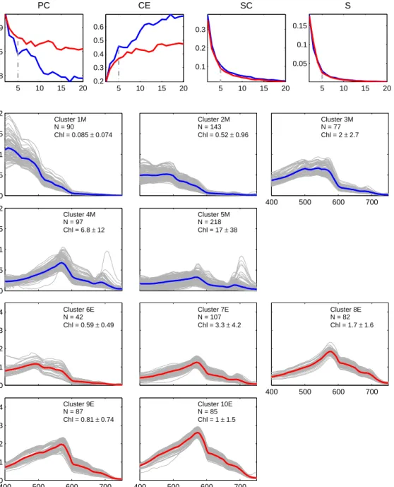
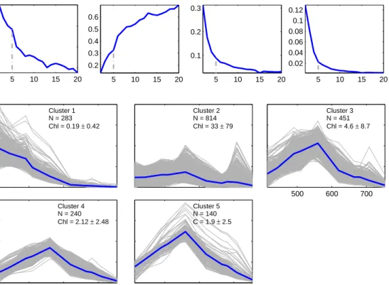
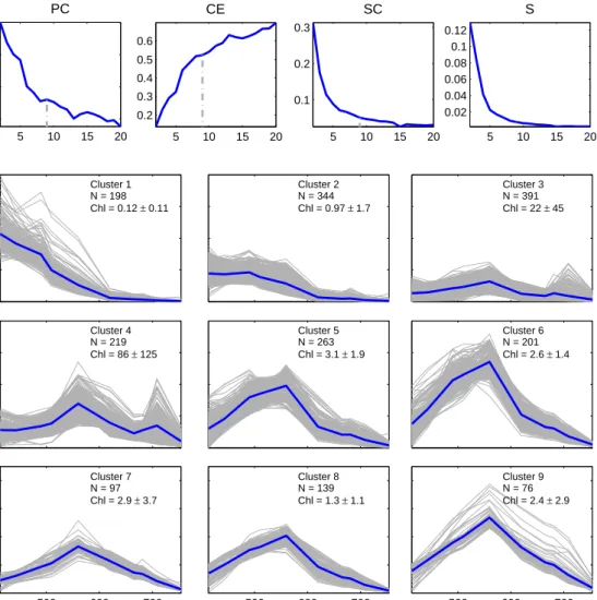
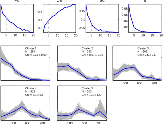
Since the optimal value for cis not known prior to clustering, a selection of four valid-ity functions were calculated for a range of cbetween 2 and 20 in order to determine the appropriate amount of clusters for the dataset. These included the Partition Coefficient, Classification Entropy, Partition Index and Separation Index as detailed below. Validity functions provide an evaluation of the performance of the clustering by means of a quant-itative measure of the quality of the outputs (Windham,1982) and the significance of the structure imposed on the data (Xie and Beni, 1991).
The Partition Coefficient (P C) (Bezdek, 1974) is an indicator of the separation of clusters and measures the overlap between clusters. The closer this value is to one the better the data were classified (Windham,1982). P C does not consider the data structure, is sensitive to the values ofcandm(Windham,1982) and thus has a tendency to decrease with increasing c(Xie and Beni, 1991). P C is defined as:
P C = 1 N c X i=1 N X j=1 (uij)2 (2.4)
where uij is the membership of thejth observation to theith cluster.
The Classification Entropy (CE) (Bezdek, 1974, 1975) measures the fuzziness of the cluster partition; a desirable outcome is close to zero. Similar toP C, theCE suffers from sensitivity to its input parameters (Windham, 1982) and has no direct connection to the geometric properties of the data (Xie and Beni, 1991). It is defined as:
CE =−1 N c X i=1 N X j=1 uijlog(uij) (2.5)
The Partition Index (SC) (Bensaid et al., 1996) is a measure of the compactness and separation of the clusters. A lower SC indicates a better partition, and it is defined as:
SC = c X i=1 PN j=1umijkxj −vik2 NiPck=1kvi−vkk2 (2.6)
whereNi is equal toPNj=1uij which is the fuzzy cardinality of each cluster. Normalization
byNi is performed to make SC insensitive to cluster sizes (Bensaid et al., 1996).
The Separation Index S (Xie and Beni, 1991), also known as the Xie-Beni Index, aims to quantify the ratio of the total variation within clusters and the minimum-distance separation of cluster centers; it favours clusters that are maximally separate from one another (Bensaid et al., 1996). S is directly related to the geometric properties of the clustering dataset and proportional to the overall average compactness and separation of clusters (Xie and Beni, 1991). S is defined as:
S = Pc i=1 PN j=1umijkxj −vik2 N ∗mini,kkvi−vkk2 (2.7)
The results from all the validity functions for each of the c from 2 to 20 were plotted, and taken into consideration when choosing the appropriate amount of clusters for each dataset. Rrs spectra were grouped into the class to which it had the highest membership;
all data related to a specific Rrs spectrum (e.g [Chl a], adg, aφ, bbφ, bbs) were also sorted
into the respective clusters to be used for further analysis. Satellite image classification
The image classification techniques are based on the concept of fuzzy logic (Zadeh,1965), and uses the methods of Moore et al. (2001, 2009, 2012, 2014). In terms of satellite imagery, the basic concept is that the observed reflectance spectrum from a pixel is given an index of similarity or membership to each cluster. The squared Mahalanobis distance Zi2 was used to quantify the closeness between the observed spectra and the cluster mean:
Zi2 = (R−Mi)tΣ−i 1(R−Mi) (2.8)
where R is the observed spectrum, Mi is the mean vector of the ith class, Σi is the
covariance matrix of the ith class, and t indicates the transpose of the vector (R−Mi).
The measure of the likelihood that a spectrum is in class iis given by the membership function fi :
fi = 1−Fn(Zi2) (2.9)
where Fn(Z2) is the cumulative χ2 distribution function with n degrees of freedom (in
describes the level of similarity between an observation and the mean vector of classi; if the observed spectrum is identical to a class mean, it will have membership value of 1. The membership function is otherwise not constrained and does not have to sum to one. The classification of MERIS images only used wavebands 2 to 10. The 412 nm band was not used during classification, as done in previous studies (Vantrepotte et al., 2012; Moore et al.,2014), since this band in MERIS data from the 3rd reprocessing is generally noisy (Smith et al., 2013; Zibordi et al.,2013; Cristina et al.,2014).
Determination of clustering database and final classes
Seven different input datasets were used during the clustering and classification scheme outlined in figure 2.1. The methodology involved a systematic process wherein the initial clustering was performed on thein situ data, whilst each subsequent step was augmented
with synthetic and/or extracted satellite data, or modified by division or normalization. In each step the relative clustering success was determined and compared to previous steps to establish the optimal clustering dataset and number of clusters for satellite image classification. These datasets are described in figure 2.2.
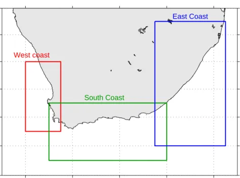
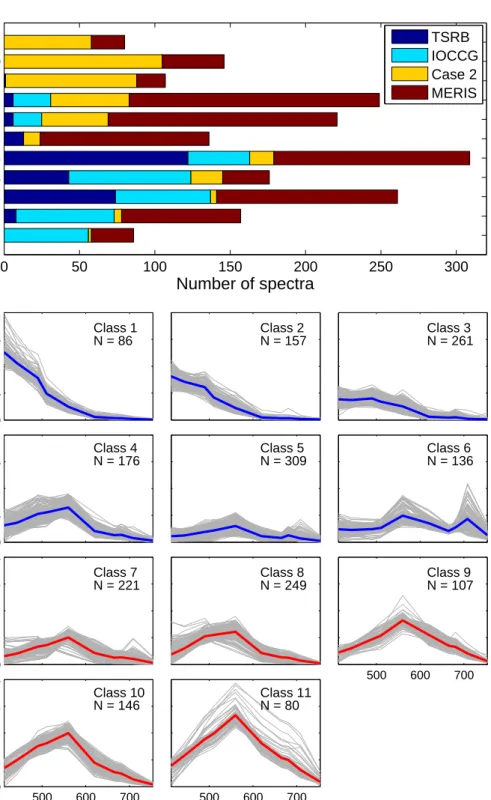
The validity functions shown in equations 2.4 to 2.7 were used to detect the optimal number of clusters for each dataset. Each dataset underwent FCM cluster analysis in order to calculate class statistics (mean and covariance matrix for each cluster), which were in turn used to classify a group of test images for three domains as represented in figure 2.3: west coast, south coast and east coast. These test images were spread over 10 years and included data from different months in an attempt to account for possible seasonal in-water and atmospheric changes which could have an impact on the classification. Ten images were selected from each domain (the dates and file names for each of the domains can be seen in tables C.1, C.2 and C.3). The average total class membership sum (A) was calculated for each image; A is defined as:
A= Pc i=1 Pn p=1fip Pn p=1p (2.10) where n is the number of valid pixels p in each image, whilst c is the number of clusters and fip is the membership function of thenth valid pixel to theith cluster. An Avalue of
close to or above 1 is desirable since it means that all or most spectra from the image were represented by one or more of the clusters of the particular dataset. The mean ( ¯A) and standard deviation ofAfrom all ten images were noted for each dataset and domain (table
Add data Add data Divide data Dataset 4M In Situ + IOCCG + Case 2 (Moderate Rrs) Hyperspectral N = 625 Dataset 4E In Situ + IOCCG + Case 2 (Elevated Rrs) Hyperspectral N = 403 Add data Add data Dataset 7 In Situ + IOCCG + Case 2 + MERIS (Normalized Rrs) Multispectral N = 1928 Dataset 5M In Situ + IOCCG + Case 2 + MERIS (Moderate Rrs) Multispectral N = 1125 Dataset 5E In Situ + IOCCG + Case 2 + MERIS (Elevated Rrs) Multispectral N = 803 Dataset 1 In Situ Hyperspectral N = 273 Dataset 2 In Situ + IOCCG Hyperspectral N = 623 Dataset 3 In Situ + IOCCG + Case 2 Hyperspectral N = 1028 Normalize data Dataset 6 In Situ + IOCCG + Case 2 + MERIS Multispectral N = 1928 Extracted satellite data Moderate Rrs N = 500 Elevated Rrs N = 400
Figure 2.2: Diagram describing each of the clustering datasets. Each block outlines the source data, spectral resolution, and the total number of spectra in each dataset. The grey arrows indicate the processes used to create subsequent datasets.
3.1 in the results); thus ¯A was used as a measure of the overall classification success of each dataset and cluster grouping per domain. A similar measure of classification success was used inMélin and Vantrepotte(2015), although they calculated their domain average of the total class membership using all available classified satellite data over the seven year study period. Several factors could affect the classification success of an image, which will be discussed later in chapters 3 and 4; however, applying iterations of different cluster sets over the same set of test images could give an indication of the improvement in the representativeness of the clustering database and the data groupings. High membership sums, and thus a highA value, indicates that one or many of the classes are represented in the database, whilst low membership indicates that the clusters are not parametrized