Sunspot
Time
Series
Forecasting
using
Deep
Learning
Mahmoud
Elgamal
Abstract:Inordertoforecastsolarcycle25, sunspotnumbers(SSN)from 1700 ∼ 2018 was used as a time series to predict the next eleven years. deep long short-term memory(LSTM) was exploited to do the forecast, first the dataset was split into training set(80%) and (20%) for the test set, the achieved accuracy led us to forecast the next eleven years. The result shows that the cycle will be from 2019 ∼ 2029 with peak at 2024.
1
Introduction
One interestingaspect of the Sun is its sunspots. Solar flares, coronal mass ejections,high-speed solarwind,and solarenergeticparticles areallformsof solar activity. All solar activity is drivenby the solar magnetic field[14]. Solar activity has important influences on allliving beings, and major tech-nologiesinthe world. As aresultof the changesinsolar activityata period of about 11 years, deviations in the near-Earth space in the interplanetary environment and the magnetosphere change the ionospheric plasma density with this period. Furthermore, changes in solar activity affect aero and space navigation,spaceflights, radars, high-frequency radio communications, and groundelectricallines. Thesechangesalso mayaffect climateandliving organisms onthe earth, including humans([1, 10, 11]). In order to estimate the sunspot cycle, sunspot number(SSN) is one of the main used indices, it is an important parameter in many scientific areas([13, 7]). The sunspot number is anactive field of research, because of its importance, difficulty of estimation, and possible applications basedon it.
A time series is a set of observations, each one being recorded at a spe-cific time. Time seriespredictionisa vitalresearch areainwhich forecasters collectand analyzehistoricalobservations toidentifyamodeltocapturethe underlying data generation process, this model will be used to predict the future values. Inthe lastdecadesArtificialneuralnetworks(ANN)proved to bea seriouscontenders tostatistical methods inforecasting. In ordertouse
ANN in forecasting tasks, it must compromise among three issues: solution complexity, forecast accuracy, and data characteristics[16].
Recurrent neural network(RNN) found to be the convenient one to achieve the above mentioned tasks, yet the majority weakness of RNN is vanish-ing/exploding gradient problem[3]. In [8, 12] this drawback was handled using long short-term memory(LSTM) algorithm as an extension to RNN. The paper is composed of: LSTM model section(2), Deep-LSTM model sec-tion(3), and simulation in section(4).
2
LSTM Model
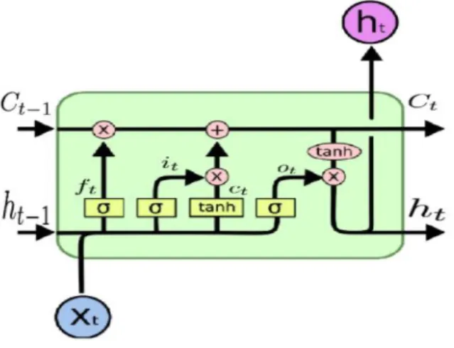
Recurrent neural networks(RNN)found to be convenient method in forecast-ing time series, as it compromises among solution complexity, forecast ac-curacy, and data characteristics[16]. RNN have the ability to store mem-ory since their current output is dependent on the previous computations. However, the major weakness of RNN is the vanishing/explosion gradient problem[5]. Long short-term memory(LSTM) were designed to overcome vanishing/explosion problem by introducing new gates which allow a better control over the gradient flow and enable better presentation of long range dependencies. Figure(1) shows the memory cell of LSTM with three gates: input gate, forget gate, and output gate.
Figure 1: LSTM cell structure.
The input sequence{x1, x2,· · · , xn} is input to RNN model using
where xt≡ input at time t,ht≡ current hidden state.
LSTM overcomes vanishing/explosion problem by introducing the gates and states of LSTM are computed as follows:
input gate: it=σ(W1i.xt+Whi.ht−1 +bi), (2) forget gate: ft=σ(W1f.xt+Whf.ht−1+bf), (3) output gate: ot=σ(W1o.xt+Who.ht−1+bo), (4) cell input: ¯ Ct= tanh(W1C.xt+WhC.ht−1 +bC), (5)
where W1i, W1f, W1o, W1C are the weight matrices connecting xt to the three
gates and the cell input,Whi, Whf, Who, WhC are the weight matrices connecting ht−1 to the three gates and the cell input, bi, bf, bo, bC are the bias terms of
the three gates and the cell input, σ represents the Sigmoid function and tanh represents the hyperbolic tangent function. Secondly, calculate the cell output state:
Ct=it∗C¯t+ft∗Ct−1, (6) where it, ft,C¯t, Ct−1 and Ct have the same dimension. Thirdly, calculate the
hidden layer output:
ht=ot∗tanh(Ct). (7)
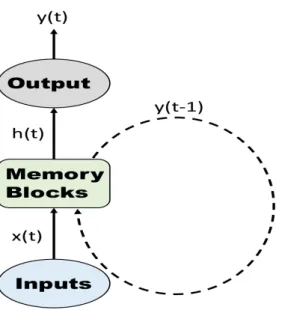
To predict the future value yt, we use the observed historical data xt as
the network input(see figure(2)). From the above LSTM calculations, ht is
obtained and hence the network output is
yt=W2.ht+b (8)
whereW2 is the weight matrix between the output layer and the hidden layer, b is the bias term of the output layer.
Figure 2: LSTM structure for time series prediction.
3
Deep LSTMs
Stacked LSTMs or Deep LSTMs were introduced by Graves[4], et al. in their application of LSTMs to speech recognition, beating a benchmark on a challenging standard problem. They found that the depth of the network was more important than the number of memory cells in a given layer to model skill. Stacked LSTMs are now a stable technique for challenging se-quence prediction problems. A Stacked LSTM architecture(figure(3)) can be defined as an LSTM model comprised of multiple LSTM layers. An LSTM layer above provides a sequence output rather than a single value output to the LSTM layer below. Specifically, one output per input time step, rather than one output time step for all input time steps.
To increase efficiency of the LSTM networks, several stacked blocks of LSTM were used in a similar way to deep recurrent network[2].
4
Experiments
The dataset of the sunspot number are freely available from world data center SILSO[15] for daily, monthly, and yearly in csv-format. The simulation run on yearly dataset from year 1700 till 2108, i.e., 318 years.
4.1
Forecasting Accuracy Errors
To measure forecast accuracy and performance evaluation, the commonly used measures are[6]:
• Root Mean Squared Error(RMSE) easy to interpret your model accu-racy written as:
RMSE = v u u t 1 n n X i=1 yi−yˆi 2
• Another commonly used one is Root Mean Square Percentage Er-ror(RMSPE) RMSPE = v u u t 1 n n X i=1 yi−yˆi yi 2 ×100
• MAPE refers to Mean Absolute Percentage Error, which is
MAPE = 100 n n X i yi−yˆi yi
where yi is the true value(observation) and ˆyi is the predicted value.
4.2
Results
The SSN dataset from 1700 ∼ 2018 was split into 80% for training set and (20% ≈ 64 years) for test set. Then we run the deep LSTM program with configurations in table(1) to get the result shown in figure(4)
Table 1: Deep LSTM configurations.
No. of layer No. of hidden units in each layer No. of Epochs RMSE RMSPE MAPE
Figure 4: SSN and their forecasts.
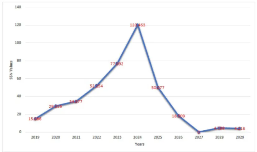
It is important to predict the next solar cycle, so the deep LSTM model run to predict the future eleven years and the results shown in figure(5) and table(2). It is clear that solar cycle 25 will have a peak SSN of 120 at year 2024.
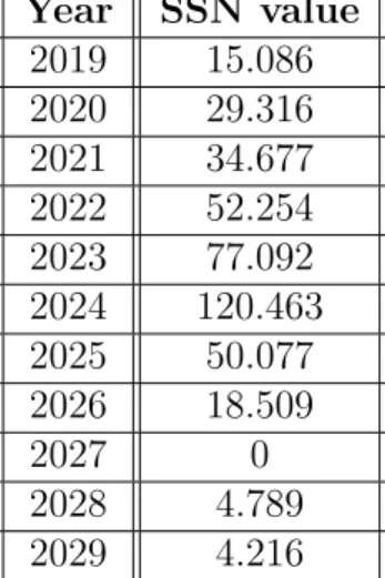
Table 2: SSN numbers and their predicted values. Year SSN value 2019 15.086 2020 29.316 2021 34.677 2022 52.254 2023 77.092 2024 120.463 2025 50.077 2026 18.509 2027 0 2028 4.789 2029 4.216
5
Conclusion
In this paper, solar cycle 25 was studied using deep LSTM, first data split into training/test sets with 80%/20% and after choosing the right parameters it was run to predict the next solar cycle.
References
[1] L. A. Aguirre, C. Letellier, and J. Maquet , Forecasting the Time Series of Sunspot Numbers, Solar Physics volume 249, pages103–120(2008). [2] j. Brownlee, Stacked Long Short-Term Memory Networks, 2019.
[3] Bayer, J. Simon, learning sequence representations, Technischen Univer-sit¨at M¨unchen, 2015.
[4] A. Graves, A. R. Mohamed, and G. Hinton, Speech recognition with deep recurrent neural networks. In Proc. International Conference on Acous-tics, Speech and Signal Processing 6645–6649 (2013).
[5] S. Hochreiter, “The Vanishing Gradient Problem During Learning Recur-rent Neural Nets and Problem Solutions”, International Journal of Un-certainty, Fuzziness and Knowledge-Based SystemsVol. 06, No. 02, pp. 107-116 (1998).
[6] R. J. Hyndman, and A. B. Koehler Another look at measures of forecast accuracy,International Journal of Forecasting 22 (2006) 679 – 688. [7] K.B. Kim, J.H. Kim, H.Y. Chang, Do Solar Cycles Share Spectral
Prop-erties with Tropical Cyclones that Occur in the Western North Pacific Ocean?, J. Astron. Space Sci. 35, 151, 2018.
[8] Pascanu, Razvan, T. Mikolov, On the difficulty of training recurrent neu-ral networks, Proceedings of the 30th International Conference on Ma-chine Learning(3), volume 28, 2013, pp. 1310-1318.
[9] J. Patterson, A. Gibson, Deep Learning. A Practitioner’s Approach; O’Reilly Media, Inc.: Sebastopol, CA, USA, 2017; pp. 150–158.
[10] W. D. Pesnell, Predictions of Solar Cycle 24, Solar Physics volume 252, pages209–220(2008).
[11] K. Petrovay, Solar Cycle Prediction, Living Reviews in Solar Physics volume 7, Article number: 6 (2010).
[12] J. Sutskever, Training recurrent neural networks, university of Toronto,PhD thesis, 2012.
[13] S. Sagir, S. Karatay, R. Atici, A. Yesil, O. Ozcan, The relationship between the Quasi Biennial Oscillation and Sunspot Number, Adv. Space Res. 55, 106.,2015.
[14] What is solar activity?, National Aeronautics and Space Administration, 2017.
[15] World Data Center for the production, preservation and dissemination of the international sunspot number, http://www.sidc.be/silso/datafiles, 2019.
[16] G. Zhang, B.E. Patuwo, M. Y. Hu, Forecasting with artificial neural net-works:: The state of the art, International Journal of Forecasting Volume 14, Issue 1, 1 March 1998, Pages 35-62.