Krill herd support vector regression and heterogeneous autoregressive leverage: evidence from forecasting and trading commodities

Stasinakis, C., Sermpinis, G., Psaradellis, I., and Verousis, T. (2016) Krill

herd support vector regression and heterogeneous autoregressive leverage:

evidence from forecasting and trading commodities. Quantitative Finance,

16(102), pp. 1901-1915. (doi:10.1080/14697688.2016.1211800)

This is the author’s final accepted version.

There may be differences between this version and the published version.

You are advised to consult the publisher’s version if you wish to cite from

it.

http://eprints.gla.ac.uk/122457/

Deposited on: 16 August 2016

Enlighten – Research publications by members of the University of Glasgow http://eprints.gla.ac.uk

1

Krill Herd Support Vector Regression and Heterogeneous Autoregressive Leverage: Evidence from Forecasting and Trading Commodities.

Charalampos Stasinakis* Georgios Sermpinis** Ioannis Psaradellis*** Thanos Verousis****

Abstract

In this study a Krill Herd - Support Vector Regression (KH-vSVR) model is introduced. The Krill Herd (KH) algorithm is a novel metaheuristic optimization technique inspired by the behaviour of krill herds. The KH optimizes the SVR parameters by balancing the search between local and global optima. The proposed model is applied to the task of forecasting and trading three commodity Exchange Traded Funds (ETFs) on a daily basis over the period 2012-2014. The inputs of the KH-vSVR models are selected through the Model Confidence Set (MCS) from a large pool of linear predictors. The KH-vSVR’s statistical and trading performance is benchmarked against traditionally adjusted SVR structures and the best linear predictor. In addition to a simple strategy, a time-varying leverage trading strategy is applied based on Heterogeneous Autoregressive (HAR) volatility estimations. It is shown that the KH-vSVR outperforms its counterparts in terms of statistical accuracy and trading efficiency, while the leverage strategy is found to be successful.

* University of Glasgow Business School, University of Glasgow, Adam Smith Building, Glasgow, G12 8QQ, UK ([email protected])

** University of Glasgow Business School, University of Glasgow, Adam Smith Building, Glasgow, G12 8QQ, UK ([email protected])

*** Institute for Risk and Uncertainty, University of Liverpool, Liverpool, L697ZH, UK ([email protected])

**** Newcastle University Business School, Newcastle University, NE14SE, UK

([email protected])

Keywords

2

1. Introduction

Commodities are in the centre of the interest for policy makers, market participants and academic researchers. After the rollercoaster in the commodity markets of 2007-2008, obtaining future expectations of commodity prices became a trivial task (Arezki et al., 2014; Chevallier et al., 2014). Hence the literature on commodity predictability is extensive and contradicting (see amongst others Chen et al. (2010), Dunis et al. (2013), Chinn et al. (2014) and Gargano and Timmermann (2014)).

Until the advent of commodities Exchange Trade Funds (ETFs) in 2003, commodity trading was thought to be exclusive to more “sophisticated” institutional investors through physical purchasing, future contracts and long-term agreements. The introduction of commodity ETFs after 2003 made the commodity markets more regulated, transparent and liquid (Mazzilli and Maister, 2006). These ETFs enabled ordinary investors to buy and sell commodities through regular brokerage accounts. Although, the advantages of ETF trading over “conventional trading” are well documented (Dolvin, 2010), the commodity ETF literature is limited. Most researchers focus on explaining why investors and portfolio managers would prefer to include commodities in their portfolios, rather than evaluating their trading performance per se (Narayan et al., 2013). Similarly, the forecasting applications mentioned above analyse commodities through their spot prices and not through commodity ETF prices. To the best of our knowledge, there are only a handful of studies that are forecasting ETF prices. Dunis et al. (2013) apply non-linear models to forecast and trade the SPDR Gold Shares Fund (GLD) in order to model the gold miner spread. In a similar study, Haugom et al. (2014) forecast the volatility in US oil market through the US Oil Fund (USO).

Financial series are very noisy and non-linear, which makes the calibration of financial models a difficult task. One popular way to overcome this is the application of heuristic optimization techniques (Gilli et al., 2008; Aguilar-Rivera et al., 2015). Metaheuristics are a superior class of heuristics, since they are less computationally demanding and can avoid local optima and over-fitting (Van Breedam, 2001). Their main advantage is that they achieve a trade-off between intensification (local search) and randomization (global search) by intelligent selection of random variables, without being problem dependent (Talbi, 2009). Most of metaheuristics are inspired by activities appearing in nature, like the evolution of species or swarm movement behavior (see amongst others Liang et al. (2006), Yang (2010), Yang and Gandomi (2012) and Li et al. (2014)). Krill Herd algorithm (KH) is a novel bio-inspired metaheuristic method proposed by Gandomi and Alavi (2012). The intuition of the algorithm is the herding behavior of krill individuals. Its objective functions are the minimum distances of krill from the food location and the location of the highest density of the herd. In that way, every krill’s position is approximated through a time-dependent function based on three motions, the movement induced by other individuals, the foraging motion and a random physical diffusion. In KH the

3

derivative information is not necessary because it uses a stochastic random search rather than a gradient search. Additionally, KH requires the fine tuning of only one parameter in contrast to other metaheuristics algorithms, such as the particle swarm optimization and the harmony search. Gandomi and Alavi (2012) and Wang et al. (2014) compare KH’s efficiency to the most popular metaheuristics optimization models. Their results suggest that KH presents a superior performance.

Support Vector Regressions (SVRs) are non-linear data-adaptive regression techniques, expanding the original classification models widely known as Support Vector Machines (SVMs). Their success in financial forecasting tasks is authenticated through numerous studies. For example, Tay and Cao (2001) apply SVMs and SVRs in forecasting time series and they conclude that these techniques outperform tradition neural network models. The SVRs’ performance is also examined in the study of Lu et al. (2009), who compare the forecasting results of SVR with random walks over daily stock prices. Their results confirm the SVRs’ superiority. Hsu et al. (2009) and Lin and Pai (2010) successfully use SVRs to forecast financial indices and business cycles respectively. Yeh et al. (2011) suggest that SVR performance is increasing when a multiple-kernel approach is adopted. Their proposed SVR structure is able to robustly forecast daily stock prices from the Taiwan Capitalization Weighted Stock Index. Rosillo et al. (2014a) and Rossillo et al. (2014b) apply SVMs in S&P 500 and VIX indices respectively. Their results indicate that the SVMs provide higher Sharpe ratios than naive or simple buy-and-hold strategies. Recently, Yao et al. (2015) compare SVR with several other statistical techniques, when applied to the task of predicting losses from corporate bond defaults. The authors conclude that SVR models substantially outperform all other statistical models in terms of both model fit and out-of-sample predictive accuracy.

The main drawback of the SVR is its parametrization process. On the one hand, forecasts are highly sensitive to the SVR’s parameters while on the other hand there is no formal theory behind their selection. In the relevant literature, researchers apply simple cross validation or grid search techniques. In this study, a KH algorithm is applied to the task. The hybrid Krill Herd - Support Vector Regression (KH-vSVR) algorithm should be able to exploit the merits of the KH optimization and provide superior forecasts. The performance of the proposed algorithm is benchmarked against two traditional SVR models optimized by 5 cross validation and grid search. To the best of our knowledge, the proposed hybrid SVR structure does not exist in the literature.

Except the SVR parameters, the practitioner needs to specify the inputs of the algorithm. This choice is usually based on objective criteria and the practitioner’s beliefs on the series under study. In this study, a large pool of potential inputs (individual forecasts) is generated in the in-sample period. The pool consists of linear predictors that are commonly used by technical analysts and traders (Park and Irwin, 2007) (see appendix A). In order to reduce the dimensions of the potential input vectors, the Model

4

Confidence Set (MCS) procedure proposed by Hansen et al. (2011) is applied. Once the optimal input vectors are selected, they are then fed to the SVR models. The best predictor in the in-sample will also act as benchmark to the SVR models.

All models are applied to the task of forecasting and trading three commodity ETFs on a daily basis over the period 2012-2014. The selected ETFs are the USO, GLD and iShares Silver Trust Fund (SLV) which track West Texas Intermediate oil, the gold bullion and the silver bullion price, respectively. ETFs offer to investors the opportunity to trade commodities with transaction costs below 0.50% per annum. The KH-vSVR forecasts and its benchmarks are evaluated through simple statistical measures, the Diebold-Mariano (DB) (1995) and the Pesaran-Timmermann (PT) (1992) test. The Giacomini-White (GW) (2006) specification tests if the generated forecasts are free from the data snooping bias. The financial evaluation of the algorithms under study is examined through a simple trading application and two basic trading measures (the annualized return and the information ratio). In order to further improve the profitability of our models, a time-adaptive leverage based on the Heterogeneous Autoregressive (HAR) model proposed by Corsi (2009) is introduced. The leverage is based on the notion that high volatility is associated with low returns.

In the empirical results, all models under study are capable of producing profitable forecasts. The KH-vSVR presents the best performance and outperforms its benchmarks in all statistical and trading measures retained. The trading performance of SVR models seems robust in the first months of the out-of-sample but it deteriorates in the second half of the 2014. Finally, we note the introduced leverage is successful as it increases the profitability of the models.

The rest of the paper is organized as follows. Section 2 provides a detailed description of the dataset while a theoretical background on the SVR is given in Section 3. The KH-vSVR algorithm explanation follows in Section 4. Its benchmarks and the SVR input selection process is outlined in Section 5. The statistical and trading performance of all models is presented in sections 6 and 7 respectively, while the concluding remarks are provided in Section 8. The appendix includes the summary of the SVR potential inputs, the technical characteristics of KH and the mathematical formulas for the statistical and trading measures retained.

2. Dataset

ETFs enable investors to trade assets with very low transaction costs. Their advantages for traders are well documented (see amongst others Avellaneda and Lee (2010), Dolvin (2010) and Marshall et al. (2013)). This study is focusing on three commodity ETFs, namely the United States Oil fund (USO), the SPDR Gold Shares (GLD) and the iShares Silver Trust (SLV). USO, GLD and SLV track the price

5

movements of oil, gold and silver respectively. All three ETFs are characterised by high liquidity and high volume of assets. Their details are presented in Table 1 below.

Table 1: The ETFs under study

ETF(TICKER) TRACKING EXPENSE RATIOS

United States Oil Fund (USO) Price of West Texas Intermediate light, sweet crude oil 0.45% per annum SPDR Gold Shares Fund(GLD) Price of gold bullion 0.40% per annum iShares Silver Trust Fund (SLV) Price of silver bullion 0.50% per annum

In this study, all models are applied in the task of forecasting the one day ahead logarithmic returns of the three ETFs. The descriptive statistics of the return series are shown in the following table:

Table 2: Descriptive statistics

We note that the three returns series exhibit slight negative skewness and positive kurtosis. The Jarque-Bera statistic confirms that the commodities return series under study are non-normal at the 99% confidence level. The Augmented Dickey-Fuller (ADF) reports that the null hypothesis of a unit root is rejected at the 99% confidence level for all ETFs.

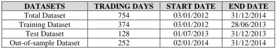
The period under study and the relevant datasets are presented in Table 3.

Table 3: The total dataset

Note: The in-sample period is the sum of the training and test datasets.

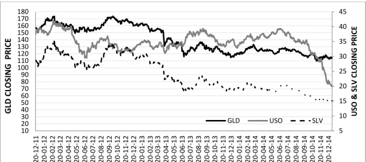
All models are optimized in the in-sample and their forecasts are evaluated in the out-of-sample. Figure 1 presents the performance of the three ETFs during the period of 3rd January 2012 to 31st December 2014. TICKER USO GLD SLV Mean -0.000831 -0.000386 -0.000771 Standard deviation 0.013981 0.011078 0.017559 Skewness -0.290346 -0.987861 -0.601902 Kurtosis 6.700746 11.45286 9.498665 Jarque-Bera (p value) 0.0000 0.0000 0.0000 ADF (p value) 0.0000 0.0000 0.0000

DATASETS TRADING DAYS START DATE END DATE

Total Dataset 754 03/01/2012 31/12/2014 Training Dataset 374 03/01/2012 28/06/2013 Test Dataset 128 01/07/2013 31/12/2013 Out-of-sample Dataset 252 02/01/2014 31/12/2014

6

Figure 1: The commodity ETFs under study

All models are optimized in the in-sample and their forecasts are evaluated in the out-of-sample.

3. Theoretical Background

Support Vector Machines (SVMs) are common classification techniques applied in machine learning and data mining. They apply the structural risk minimization principle in order to obtain good generalization on a limited number of learning patterns. Support Vector Regression (SVR), introduced byVapnik (1995), is one class of SVMs. SVRs are established as a robust technique for constructing data-driven and non-linear empirical regression models (Witten and Frank, 2005).

3.1 SVR

Considering the training data {(x1,y1), (x2,y2)…, (xn, yn)}, where xi∈ ⊆X R y, i∈ ⊆Y R i, =1...n and n

the total number of training samples, then the SVR function can be specified as:

( ) T ( )

f x =w ϕ x +b (1) φ(x) is the non-linear function that maps the input data vector x into a feature space where the training data exhibit linearity (see Figure 2c) while w and b are estimated by minimizing the regularized risk function: 5 10 15 20 25 30 35 40 45 10 20 30 40 50 60 70 80 90 100 110 120 130 140 150 160 170 180 20 -12 -11 20 -01 -12 20 -02 -12 20 -03 -12 20 -04 -12 20 -05 -12 20 -06 -12 20 -07 -12 20 -08 -12 20 -09 -12 20 -10 -12 20 -11 -12 20 -12 -12 20 -01 -13 20 -02 -13 20 -03 -13 20 -04 -13 20 -05 -13 20 -06 -13 20 -07 -13 20 -08 -13 20 -09 -13 20 -10 -13 20 -11 -13 20 -12 -13 20 -01 -14 20 -02 -14 20 -03 -14 20 -04 -14 20 -05 -14 20 -06 -14 20 -07 -14 20 -08 -14 20 -09 -14 20 -10 -14 20 -11 -14 20 -12 -14 US O & S LV CL OS IN G P RICE GL D C LO SIN G PR IC E GLD USO SLV

7 2 1 1 1 ( ) ( , ( )) 2 n i i i R C C L y f x w n = ε =

∑

predicted value at the same period. The ε-sensitive loss Lε function (see Figure 2b) is defined as: 0 | ( ) | ( , ( )) , | ( ) | i i i i i i if y f x L y f x y f x if other ε _ε ε − ≤ ε  =_ ≥ 0 − −  (3)

Equation (3) identifies the predicted values that have at most ε deviations from the actual values yi,

while the ε parameter defines a ‘tube’ (see Figure 2a). The two variables,

ξ

i

ξ represent the distance of the actual values from the upper and lower bound of the ‘tube’ respectively.

Figure 2: a) The ε-tube b) The plot of the ε-sensitive loss function c) The mapping procedure by φ(x)

The goal is to solve the following argument:

Minimize * 2 1 1 ( ) 2 n i i i C ξ ξ w = + +

∑

The quadratic optimization problem of equation (4) is transformed in a dual problem and its solution is based on the introduction of two Lagrange multipliers _, *

i i

a a and mapping with a kernel function

( , )i K x x : * 1 ( ) ( ) ( , ) n i i i f x a a K x x b i= =

∑

8

The application of the kernel function transforms the original input space into one with more dimensions, where a linear decision border can be identified. In this study, the Gaussian Radial Basis Function (RBF) for all SVRs is applied. A RBF kernel is in general specified as:

2

( , )_i exp( _i ), 0

K x x = −γ x −x γ >

(6)

where, γ is the variance of the kernel function. RBF’s requires only one parameter to be optimized (the γ) while it provides good forecasting results in similar SVR applications (Lu et al., 2009; Yeh et al., 2011).

Factor b in equation (5) is computed following the Karush-Kuhn-Tucker conditions. A detailed mathematical explanation of the solution can be found in Vapnik (1995). Support Vectors (SVs) are called all the xi that contribute to equation (5), thus they lie outside the ε-tube, whereas non-SVs lie

within the ε-tube. Increasing ε leads to less SVs’ selection, whereas decreasing it results to more ‘flat’ estimates. The norm term w2characterizes the complexity (flatness) of the model and the term

* 1 ( ) n i i i ξ ξ =  ₊    



∑

of the parameter C satisfies the need to trade model complexity for training error and vice versa (Cherkassky and Ma, 2004).

The v-SVR algorithm can be used to make the optimization task easier, by encompassing the ε parameter in the optimization process and controls it with a new parameterv∈(0,1). In v-SVR the optimization problem transforms to:

Minimize * 2 1 1 1 ( ) 2 n i i i C v w n ε ξ ξ =  _{+ +} ₊   

∑

The methodology remains the same as in ε-SVR and the solution takes a similar form:

* 1 ( ) ( ) ( , ) n i i i f x a a K x x b i= =

∑

Based on the ‘v-trick’, as presented by Schölkopf et al. (1999), increasing ε leads to the proportional

increase of the first term of *

1 1 ( ) n i i i v n ε ξ ξ =  _{+ +}   



∑

fraction of points outside the ε-tube. So v can be considered as the upper bound on the fraction of errors. On the other hand, decreasing ε leads again to a proportional change of the first term, but also the second term’s change is proportional to the fraction of SVs. That means that ε will shrink as long

9

as the fraction of SVs is smaller than v, therefore v is also the lower band in the fraction of SVs. For a more detailed mathematical analysis of the above solutions see Vapnik (1995).

The SVR performance is highly sensitive to the selected SVR parameters. Although v-SVR makes this process less computationally demanding compared to ε-SVR, the practitioner still needs to fine tune the C, v and kernel function parameter (in this case γ). Researchers commonly apply statistical approaches such as grid search (v-SVR1) and 5-fold cross validation (v-SVR2) to tackle this problem (see amongst others Duan et al. (2003), Min and Lee (2005) and Ding et al. (2008))

4. Krill Herd Support Vector Regression (KH-vSVR)

In this Section, we propose a hybrid Krill Herd – Support Vector Regression that embodies a KH algorithm for optimal parameter selection to the v-SVR process, as shown in Section 3. The KH algorithm, as presented by Gandomi and Alavi (2012), is an innovative metaheuristic optimization technique that simulates the herding behavior of the Antarctic krill. More specifically, the algorithm is inspired by the individual responses of krill, when sea predators are attacking the herd. When this happens, the krill herd density decreases because of the krill dispersion from the attack. After the attack the krill gather again through a mean-reversion process. The main element of this process is that herd density will start increasing again by krill individuals sensing nearby krill, without deviating much from the optimal path to reach food, as set before the attack.

Within this framework, Gandomi and Alavi (2012) propose that the position (P) of each krill in the search space is influenced by the movement induced by other krill (M), the foraging action (F) and the random diffusion (RD). All these motions can be summarized in one Lagrangian formulation for every krill j: j j j j dP M F RD dt = + + (9)

The new movement motion M t+1 of each krill j is calculated as:

1 max arg t t j j M loc t j j j M M eff k

eff eff eff

+  = + M      = +     (10) Where:

• Mmax: the maximum induced speed

• k_M∈[0,1]: the inertia weight of the motion

• t

j

10

• eff_j: the direction of the motion

• loc

j

eff , targ

j

eff : the local effect by neighbor krill and the target direction effect by the best individual krill.

Gandomi and Alavi (2012) suggest that the local search of the algorithm is based on an attractive/repulsive tendency between individual krills. The neighbor krills are identified through a sensing distance from the jth one:

_{, k '} ' 1 (1 / N ) k N s j j j j d P P = =

∑

The new foraging motion F t+1 of every krill j is also calculated on the basis of two factors, namely the food location and its previous experience in locating a correct food position:

1 t t j F j F j food best j j j F V floc k F

floc floc floc

+  = +      = +     (12) where:

• VF: the foraging speed

1

• k_F∈[0,1]: the inertia weight of the motion

• t

j

F : the previous foraging motion

• floc_j: the location of the food

• food

j

floc , best

j

floc : the food attractive and the effect from the best food-locating jth krill so far The food attraction is defined to provide global optima for the krill swarm. The third motion RD of krills is calculated as a maximum diffusion speed RDmaxand a random directional vector δ with values between 1 and -1. In other words:

RD=RDmaxδ (13)

Equations (10) and (12) suggest the future krill motion towards the optimal position by performing two parallel local and global strategies, something that makes the KH algorithm very robust. Krill continue their local search until the herd density increases. This is approximated with equation (10). Once the density is increased, more and more krill orientate to food rather than the nearby krill as per equation (12). These two strategies provide the fitness values for several effective factors that induce an attractive/repulsive motion response to each krill. The equation (18) performs a random search in the

1

The maximum induced speed of equation (15) and the foraging speed of equation (17) are set to 0.01 and 0.02 ms-1

11

proposed search space, diffusing any potential biased motion responses to the herd (either towards food locations or neighboring sensed krill). For more details on the approximation of these values, please refer to the extensive mathematical steps of Gandomi and Alavi (2012). Based on the above, the position Pj of each krill is a time t+Δt is given as:

(

)

∑

• NP: the number of parameters optimized (in our case NP=3)

• UpB LowB_r, _r: the upper and lower bounds of the parameters

The Δt practically is the only parameter that needs fine tuning. This is the striking advantage of the method compared to other more complicated metaheuristics approaches. In the KH-vSVR optimization, the practitioner needs to predefine three parameters (C, v and γ). Τhe potential three-dimensional search space is defined by the range of the bounds of each parameter. Setting Zcr at values

lower than 1, allows a careful search of the space by the krill individuals. In addition, kM and kF are

initially set high (0.9). The reason for that is that the krill behavior suggests that herd individuals at an initial point (predator attack) tend to focus on exploration of the search space and then its exploitation. Based on the suggestion of Gandomi and Alavi (2012) these parameters should linearly be decreased to 0.1 at the end in order to encourage the krill to start exploiting the search space. Finally, two genetic reproduction mechanisms (mutation and crossover) are implemented in order to further improve the performance of the krill positions.

The KH algorithm is optimized based on a fitness function. In this application, the fitness function aims to minimize the RMSE:

Fitness=1 / (1+RMSE) (15)

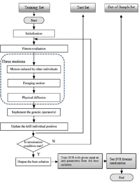
The aim of the algorithm is to maximize equation (15). The KH-vSVR algorithm is trained in the training sub-period and its performance is evaluated in the test sub-period. Figure 4 below provides the flowchart of the proposed methodology, while the training specification and the pseudo-code of the KH algorithm is given in appendix Section B.

12

Figure 4: KH-vSVR flowchart

5. Input selection and benchmark models

The SVR inputs are selected from a pool of potential linear predictors generated in the in-sample. This set of inputs includes Simple Moving Averages (SMAs), Exponential Moving Averages (EMAs), Autoregressive terms (ARs), Autoregressive Moving Average models (ARMAs), Rate of Change Indicators (ROCs) and a Pivot Point Indicator (PPI). These predictors create a pool of four hundred and seventy individual (470) models in total for each of the three ETF series. All these models have been successfully applied in financial forecasting applications and are commonly used by technical analysts (Park and Irwin, 2007). The proposed models will combine the best predictors in order to generate superior out-of-sample performance. A short summary of these individual forecasting models is provided in Appendix A.

In order to cope with the dimension of the input vector, we perform a statistical procedure to select an optimal set of informationally efficient set of inputs. This process is the MCS test proposed by Hansen

13

et al. (2011). The test selects a random data-dependent set of best forecasting models, considering that there can be information limitations in the provided dataset. The MCS test is able to deduce superior predictors from a full set of models, given specific criteria and confidence levels. In this research, the criterion is the MSE while the confidence level is set at 90%. The relaxed will allow us to deduct the best forecasters from the predictors’ pool in the in-sample and apply them as SVR inputs. Higher confidence level would have limit the input set to only 1 or 2 models while a lower level would have included inputs not informationally efficient. The inputs sets are presented in Table 4.

Table 4: SVR sets of inputs

Note: The inputs highlighted with bold present the best individual in-sample statistical performance in terms of RMSE.

ETF SELECTED INPUTS TOTAL

USO SMA (7), AR(3), AR(5), ARMA (1, 4), ARMA (2, 6), ARMA (2, 8), ROC(5) 7

GLD SMA(12), EMA(5), AR(6), AR(8), ARMA( 1, 7), ARMA(4, 11) 6

SLV SMA(3), SMA(5), SMA(8), EMA(5), EMA(9), AR(4), AR(7), AR(10), ARMA (1, 9), ARMA(3,14) 10

The above sets will act as inputs to the KH-vSVR, v-SVR1 and the v-SVR2 models. The best predictor will also be included in the statistical and trading evaluation. It will allow us to establish if the SVR models actually improve the forecasting performance and to which extent. The best predictors for the the USO, GLD and SLV series are an ARMA(1,4), a SMA(12) and an ARMA(1,9) respectively.

In terms of the benchmark models applied in this study, the best individual predictors are used as a starting point. Those models, as expected, are included in the final SVR inputs selected through the MCS test. Using the best individual predictors as a benchmark allows us to establish if the forecast combinations actually further improve statistical accuracy, as proposed by Timmermann (2006). Then, two SVR forecast combination models, v-SVR1 and the v-SVR2, are compared with the proposed KH-vSVR algorithm.

6. Statistical evaluation

This Section provides the statistical performance of all models under study. Initially, the statistical accuracy of the obtained forecasts is evaluated based on the RMSE (see appendix C) and the Pesaran-Timmermann (PT) (1992) test. The PT test is used to examine whether the directional movements of the real and forecast values are in step with one another. The null hypothesis is that the model under study has no power on forecasting the relevant ETF return series. The in-sample and out-of-sample results are summarized in Table 5.

14

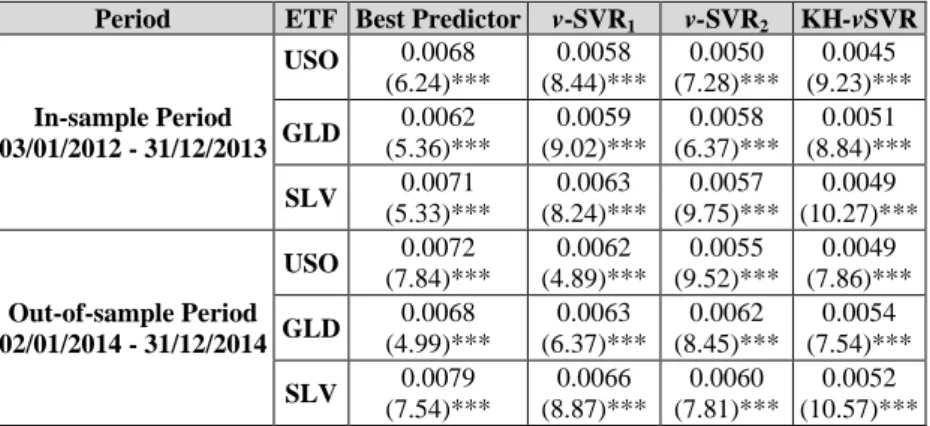
Table 5: In-sample and out-of-sample statistical performance

Note: The table reports the RMSE values of each SVR forecast, while the PT statistics are in the parenthesis. ARMA(1,4), SMA(12) and ARMA(1,9) are the best predictors for USO, GLD and SLV series respectively. *** denotes that the null hypothesis is rejected at 1% significance level.

The above results show that the models’ statistical ranking is consistent across all ETFs series and periods under study. The proposed KH-vSVR is found to have the best statistical results compared to all models. The v-SVR2 is the second best model in terms of the statistical measures retained. All SVR models outperform the best predictor in each commodity ETF under study. The PT statistics indicate that all models are capable of capturing the directional movements of the three ETF return series in-sample and out-of-in-sample. Based on the above, the KH-vSVR is the superior model in terms of statistical efficiency.

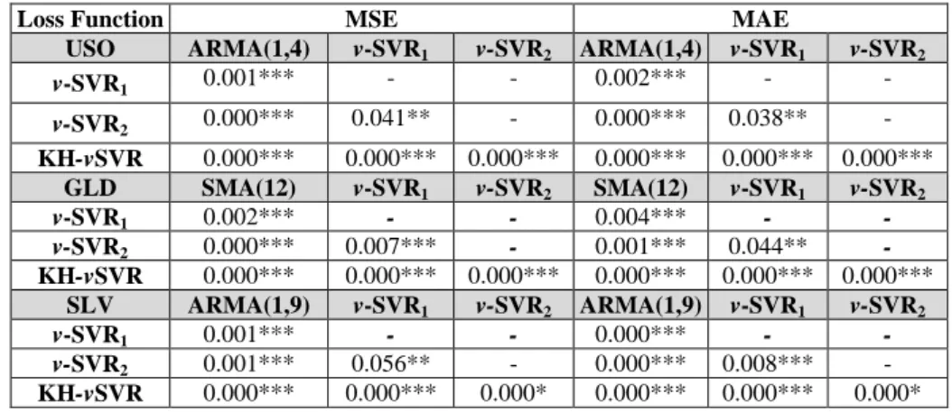
In order to further verify this outcome, the Diebold Mariano (DM) (1995) test is computed. The DM statistic tests the null hypothesis of equal predictive accuracy between two forecasts. In this exercise, the DM test is applied to couples of out-of-sample forecasts (KH-vSVR vs. other benchmark model) using the MSE and MAE loss functions. A negative realization of the DM value indicates that the KH-vSVR forecast is more accurate than the competing forecast. Table 6 summarizes the results for the DM statistic.

Table 6: Summary results of DM statistic for MSE and MAE loss functions.

Note: The values in the parentheses are the calculated DM statistics. *** denotes that the null hypothesis is rejected at 1% significance level. The results refer to the out-of-sample period (02/01/2014 – 31/12/2014).

Period ETF Best Predictor v-SVR1 v-SVR2 KH-vSVR

In-sample Period 03/01/2012 - 31/12/2013 USO 0.0068 (6.24)*** 0.0058 (8.44)*** 0.0050 (7.28)*** 0.0045 (9.23)*** GLD 0.0062 (5.36)*** 0.0059 (9.02)*** 0.0058 (6.37)*** 0.0051 (8.84)*** SLV 0.0071 (5.33)*** 0.0063 (8.24)*** 0.0057 (9.75)*** 0.0049 (10.27)*** Out-of-sample Period 02/01/2014 - 31/12/2014 USO 0.0072 (7.84)*** 0.0062 (4.89)*** 0.0055 (9.52)*** 0.0049 (7.86)*** GLD 0.0068 (4.99)*** 0.0063 (6.37)*** 0.0062 (8.45)*** 0.0054 (7.54)*** SLV 0.0079 (7.54)*** 0.0066 (8.87)*** 0.0060 (7.81)*** 0.0052 (10.57)***

ETF Loss Function Best Predictor v-SVR1 v-SVR2

USO MSE (−9.22)*** (−7.33)*** (−5.86)*** MAE (−7.32)*** (−6.14)*** (−5.75)*** GLD MSE (−8.41)*** (−7.21)*** (−3.28)*** MAE (−9.05)*** (−7.53)*** (−4.87)*** SLV MSE (−6.57)*** (−6.28)*** (−5.86)*** MAE (−8.19)*** (−7.27)*** (−6.37)***

15

Based on the above table’s results, the null hypothesis of equal predictive accuracy is rejected for all comparisons and for both loss functions at 1% significance level. Moreover, the statistical superiority of the KH-vSVR forecasts is validated, as all the DM statistic realizations are negative. Finally, v-SVR2 is found to have the closest forecasts to the proposed algorithm.

The validity of the forecasting models is evaluated through the unconditional Giacomini-White (GW) (2006) test for the out-of-sample predictive ability testing. The null hypothesis of the GW test represents the equivalence in forecasting accuracy between two forecasting techniques, according to a general loss function. The sign of the test statistic specifies which model performs better. A positive realization of the GW test statistic indicates that the second model is more accurate (produces smaller average loss) than the first one (larger average loss), whereas a negative resolution specifies the opposite. The test is calculated based on the MSE and MAE loss functions. Table 7 below presents the outcomes of the GW test.

Table 7: Giacomini-White test statistics for the MSE and MAE loss functions.

Note: The table displays the p-values of the statistic under the null hypothesis that the column model shows equivalent performance compared with each row model for every ETF and loss function separately. ***, ** denote a rejection of the null hypothesis at the 1% and 5% significance level respectively. The results refer to the out-of-sample period (02/01/2014 – 31/12/2014)

The above results further authenticate our initial statistical findings. The null hypothesis of the GW test is rejected in all cases at the 5% and 1% significance levels for both MSE and MAE loss functions. That suggests that the individual best forecasts are statistically inferior to the SVR forecast combinations. Based on Tables 5, 6 and 7, we note that the v-SVR2 provides significantly better forecasts than v-SVR1. This suggests that using 5-fold cross-validation can lead to higher accuracy in the SVR process compared to the grid search method. The KH-vSVR is found to be statistically superior in all cases and comparisons with the other models. Implementing the GW test amplifies the success of the DM test, since it suggests that the DM test validity holds regardless of the models being

Loss Function MSE MAE

USO ARMA(1,4) v-SVR1 v-SVR2 ARMA(1,4) v-SVR1 v-SVR2

v-SVR1 0.001*** - - 0.002*** - - v-SVR2 0.000*** 0.041** - 0.000*** 0.038** - KH-vSVR 0.000*** 0.000*** 0.000*** 0.000*** 0.000*** 0.000*** GLD SMA(12) v-SVR1 v-SVR2 SMA(12) v-SVR1 v-SVR2 v-SVR1 0.002*** - - 0.004*** - - v-SVR2 0.000*** 0.007*** - 0.001*** 0.044** - KH-vSVR 0.000*** 0.000*** 0.000*** 0.000*** 0.000*** 0.000*** SLV ARMA(1,9) v-SVR1 v-SVR2 ARMA(1,9) v-SVR1 v-SVR2 v-SVR1 0.001*** - - 0.000*** - - v-SVR2 0.001*** 0.056** - 0.000*** 0.008*** - KH-vSVR 0.000*** 0.000*** 0.000* 0.000*** 0.000*** 0.000*

16

nested or non-nested. In that sense, GW test offers a solid protection from data snooping bias in the statistical results of this study.

7. Trading evaluation

Further to the above statistical evaluation, the utilized models are compared also in terms of trading efficiency. It is interesting to establish whether the statistical accuracy of the proposed methodology is consistent with trading profitability. Section 7.1 presents the trading performance of all models without leverage. In Section 7.2 a time-varying leverage trading strategy is introduced based on HAR volatility estimations aiming to increase the profitability of all models.

7.1. Trading performance without leverage

In this application, the trading performance of our models is evaluated with a simple trading strategy. The position is ‘long’ and ‘short, when the forecast return is positive and negative respectively. A ‘long’ or ‘short’ position means that we buy or sell respectively the ETF under study at the current price. Transaction costs can impede the success of daily trading strategies (Wyart et al., 2008). As mentioned before, ETFs offer investors the opportunity to trade with low transaction costs, especially when the selected ETFs are highly liquid as USO, GLD and SLV. Table 1 provides the expense ratios for the three commodity ETFs examined. The in-sample and out-of-sample performance of the models is presented in the Table 8. The trading performance measures are given in appendix C.

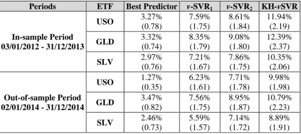
Table 8: Out-of-sample Trading Performance of every model for each ETF

Note: The table reports the annualized return after transaction costs of every model and its respective information ratio in the parenthesis. ARMA(1,4), SMA(12) and ARMA(1,9) are the best predictors for USO, GLD and SLV series respectively.

As expected, the above table results show that all models perform better in-sample than out-of-sample. The trading efficiency ranking coincides with the statistical one presented in Section 6. The KH-vSVR

Periods ETF Best Predictor v-SVR1 v-SVR2 KH-vSVR

In-sample Period 03/01/2012 - 31/12/2013 USO 3.27% (0.78) 7.59% (1.75) 8.61% (1.84) 11.94% (2.19) GLD 3.32% (0.74) 8.35% (1.79) 9.08% (1.80) 12.39% (2.37) SLV 2.97% (0.76) 7.21% (1.67) 7.86% (1.75) 10.35% (2.06) Out-of-sample Period 02/01/2014 - 31/12/2014 USO 1.27% (0.35) 6.23% (1.61) 7.71% (1.78) 9.98% (1.98) GLD 3.47% (0.82) 7.56% (1.75) 8.95% (1.87) 10.79% (2.23) SLV 2.46% (0.73) 5.59% (1.57) 7.14% (1.72) 8.89% (1.91)

17

delivers the best trading performance for all series and periods under study. On average, the proposed algorithm achieves 9.89% annualized returns and 2.04 information ratio after transaction costs in the out-of-sample period. That indicates that the suggested trading strategy benefits from the application of the KH optimization to the simple SVR process. The second best model in terms of the same trading performance measures is the v-SVR2, which presents on average out-of-sample profits and information ratio after transaction costs at the level of 7.93% and 1.79 respectively. The grid search based SVR achieves 1.47% lower profits and 0.15 lower information ratios on average, after accounting for transaction expenses. Although the best individual predictors achieve some profitability, they are always outperformed by the SVR forecast combination techniques. In terms of the commodities under study, trading GLD proves to be more profitable under the strategy without leverage. GLD trading yields on average 1.40% and 1.67% higher net profits from USO and SLV respectively.

The models’ profitability micro-structure can also be seen by the monthly decomposition of the annualized returns during the out-of-sample period. These results are provided in Table 9 below.

Table 9: Monthly Out-of-sample Trading Performance

Note: The table reports the monthly annualized returns after transaction and leverage costs of each model and ETF under study. In bold are the results that do not coincide with the previous statistical and trading ranking of the models. The last column to the right shows the total average annualized returns after transaction costs as per Table 8.

The results of Table 9 support the previous findings, since the monthly profitability of the models is in its vast majority consistent with the yearly one. The proposed methodology continues to outperform

Year 2014

ETF Models Jan Feb Mar Apr May Jun Jul Aug Sep Oct Nov Dec Average

USO ARMA(1, 4) -0.13% 1.99% 0.87% 4.90% -1.57% 4.39% 3.02% 0.63% -0.27% 0.69% -0.17% 0.87% 1.27% v-SVR1 6.47% 9.84% 10.51% 9.58% 9.18% 9.08% 7.85% -1.26% 5.63% 4.85% 4.11% -1.12% 6.23% v-SVR2 4.74% 10.85% 12.22% 9.02% 11.92% 6.57% 8.95% 8.87% 8.84% 7.42% 7.25% 6.72% 7.71% KH-vSVR 13.84% 14.75% 14.55% 13.86% 13.84% 14.47% 8.79% 9.97% 9.86% 10.57% 9.68% 9.12% 11.94% GLD SMA(12) 3.85% -1.12% 6.68% 7.52% 4.89% 3.86% 3.84% 3.28% 3.28% 2.74% 1.88% 0.97% 3.47% v-SVR1 3.75% 10.47% 10.96% 11.21% 10.25% 8.86% 8.21% 7.63% 7.25% 6.53% 5.77% -0.14% 7.56% v-SVR2 6.32% 9.86% 13.27% 10.85% 12.39% 11.56% 7.53% 9.57% 6.41% 7.21% 7.05% 5.36% 8.95% KH-vSVR 11.23%12.67% 13.55% 12.25% 13.75% 12.64% 9.84% 8.44% 9.23% 9.41% 8.84% 7.58% 10.79% SLV ARMA(1, 9) 3.58% 2.25% -2.12% 6.53% 3.84% 6.86% 3.58% 2.68% 0.94% 1.96% -0.07% -0.54% 2.46% v-SVR1 4.34% 9.84% 7.88% 7.28% 8.17% 7.23% 6.14% 5.34% 4.21% 1.44% 3.42% 1.74% 5.59% v-SVR2 6.13% 8.53% 9.67% 8.86% 10.25% 7.51% 7.32% 7.23% 6.51% 5.95% 4.22% 3.53% 7.14% KH-vSVR 8.74% 9.30% 10.74% 9.04% 12.67% 9.37% 8.74% 8.83% 7.52% 7.59% 7.84% 6.32% 8.89%

18

the two SVR counterparts with some rare exceptions (in July for USO and in August for GLD). The results of the individual models remain inferior (in most cases) and seem more erratic compared to those of the SVR forecast combinations. All models’ profits exhibit a time-varying eroding behaviour. The returns of KH-vSVR are higher and their decay smoother, which could be attributed to the success of the KH optimization. In summary, the empirical evidence of this Section suggests that the KH-vSVR is the best model in terms of trading efficiency. It would be interesting to see if this is the also the case once the leverage trading strategy of the next Section is applied.

7.2 Trading performance with HAR volatility leverage

In order to further improve the trading performance of all models, a time-varying leverage strategy is introduced. Its purpose is to avoid trading when volatility is very high, while at the same time exploit days when the volatility is relatively low. The positions, as in the previous section, are ‘long’ and ‘short, when the forecast returns are positive and negative respectively.

The volatility estimations of this study are based on the HAR model proposed by Corsi (2009). The intuition of the model is that the behaviour of traders is heterogeneous, when it comes to their trading frequency. Thus, interactions between short, medium and long-term market agents lead to a daily, weekly and monthly volatility component (partial volatilities)2. At each level of this volatility cascade, the underlying volatility component consists not only of its past observation but also of the expectation of longer horizon partial volatilities. The proposed model is defined as an additive linear structure of first-order autoregressive partial volatilities able to capture long-range dependence:

( ) ( ) ( ) ( ) ( ) ( )

(

)

lriv=β′+β′ lriv₋ +β′ lriv₋ +β′ lriv₋ +e e N σ (16)

where 𝑙𝑙𝑙𝑙(ℎ�) = 1

ℎ�∑ℎ�𝚥̂=1𝑙𝑙𝑙𝑙𝑡−𝚥̂+1 and ℎ� = (1,5,22) ′ is an index vector that depicts the daily, weekly

and monthly components of the volatility cascade.

As a first step, the previous HAR model specification is used to forecast the one day ahead realized volatility in the test and out-of-sample datasets for all ETFs (see appendix D for HAR pseudo-code). Then, following Dunis and Miao (2006), these two periods are split into six sub-periods, ranging from periods with extremely low volatility to periods experiencing extremely high volatility. Periods with different volatility levels are classified as following: firstly the average (μ) difference between the actual volatility in day t and the forecasted for day t+1 and its ‘volatility’ (measured in terms of

2

Intraday traders, speculators and hedge funds are examples of short-term agents. Commercial banks can be though as medium-term agents, while pension funds and insurance companies are long-term agents.

19

standard deviation σ) are calculated. Those periods where the difference is below μ+1σ are classified as ‘Lower high vol. periods’. Similarly, ‘Medium high vol.’ (between μ+σ and μ+2σ) and ‘Extremely high vol.’ (above μ+2σ) periods can be defined. Periods with low volatility are also defined following the same 1σ and 2σ approach, but with a minus sign. For each sub-period a leverage value is assigned starting with 0 for periods of extremely high volatility to a leverage of 2.5 for periods of extremely low volatility (leverage increases by 0.5 for each period with different levels of volatility). The leverage factors are time-varying since the parameters μ and σ are updated every one month by rolling forward the estimation period. For instance, μ and σ of the first month in the out-of-sample period are computed based on the six months of the test sub-period. The parameters of the following month are calculated based on the last five months of the test sub-period and the first month of the out-of-sample period.

In this case the cost of leverage should be accounted along with the transaction costs. This corresponds to interest payments for using additional capital. The cost of leverage is calculated at 0.56 % per annum3. The out-of-sample results derived from the above strategy are presented in Table 10 below.

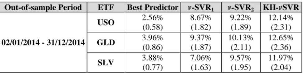
Table 10: Out-of-sample Trading Performance of every model for each ETF with leverage

Note: The table reports the annualized return after transaction and leverage costs of every model and its respective information ratio in the parenthesis. ARMA(1,4), SMA(12) and ARMA(1,9) are the best predictors for USO, GLD and SLV series respectively.

The implementation of the time-varying HAR leverage appears to be successful for all models. Across all ETFs and models, the profitability and the information ratios increase on average by 1.76% and 0.15 respectively. The KH-vSVR outperforms all benchmark models for all series. Within the leverage strategy, it achieves on average annualized returns of 12.25% and information ratio of 2.24 after accounting for transaction and leverage costs. These are significantly higher than the results attained without leverage (9.89% and 2.04). The trading ranking of the models remains the same after the application of the strategy. The v-SVR2 continues to outperform the v-SVR1, presenting on average 1.27% higher profits and 0.21 higher information ratio. The individual models’ trading performance is also positively affected by the time-varying leverage, but their profitability remains by far the lowest.

3

Interest costs are calculated by considering a 0.56% interest rate p.a. (the Euribor rate at the time of calculation) divided by 252 trading days. In reality, leverage costs are also applied during non-trading days so that we should calculate the interest costs using 360 days per year. But for the sake of simplicity, we use the approximation of 252 trading days to spread the leverage costs of non-trading days equally over the trading days. This approximation prevents us from keeping track of how many non-trading days we hold a position.

Out-of-sample Period ETF Best Predictor v-SVR1 v-SVR2 KH-vSVR

02/01/2014 - 31/12/2014 USO 2.56% (0.58) 8.67% (1.82) 9.22% (1.89) 12.14% (2.31) GLD 3.96% (0.86) 9.37% (1.87) 10.13% (2.11) 12.65% (2.36) SLV 3.88% (0.77) 7.06% (1.63) 9.57% (1.95) 11.97% (2.04)

20

It is interesting to note that trading gold with leverage now yields 0.88% and 0.91% higher returns from trading oil and silver respectively. These differences are lower from the equivalent values from the previous Section (1.40% and 1.67%). As before, Table 12 presents the monthly annualized returns after transaction and leverage costs during the out-of-sample period.

Table 11: Monthly Out-of-sample Trading Performance after leverage

Note: The table reports the monthly annualized returns after transaction and leverage costs of each model and ETF under study. In bold are the results that do not coincide with the previous statistical and trading ranking of the models. The last column to the right shows the total average annualized returns after transaction costs as per Table 11.

The above final results indicate that the leverage strategy pays dividends also when the microstructure of the returns is examined. The profits after transaction and leverage expenses appear boosted in most months of the out-of-sample period. The KH-vSVR trading superiority is once more confirmed over all benchmarks during all months. The SVR method provides higher profitability when 5-fold cross-validation is applied, except in only four cases across all months and ETFs. The application of leverage enhances the performance of the best predictors. However, using the forecast combinations of the three SVR methods yields consistently higher net profits The overall monthly decomposition of the obtained returns not only authenticates the findings of the previous Section but it also confirms the success of the HAR-based leverage strategy. It is interesting to note that under the leverage strategy, monthly losses are barely observable in contrast to the results of Table 9.

The empirical evidence presented in all sections allows us to conclude that the proposed KH-vSVR is a robust model for forecasting and trading the three exchange traded commodities under study. The

Year 2014

ETF Models Jan Feb Mar Apr May Jun Jul Aug Sep Oct Nov Dec Average

USO ARMA(1, 4) 3.34% 3.66% 2.12% 5.12% 1.44% 5.39% 3.32% 1.88% 1.78% 2.02% -0.45% 1.13% 2.56% v-SVR1 8.15% 9.55% 12.32% 9.86% 11.54% 10.86% 12.37% 6.96% 6.67% 6.31% 5.49% 3.97% 8.67% v-SVR2 9.36% 10.98% 11.53% 10.37% 10.42% 11.05% 13.26% 7.41% 6.98% 7.38% 6.38% 5.53% 9.22% KH-vSVR 12.67% 13.64% 13.68% 12.97% 14.54% 13.99% 14.55% 12.27% 10.08% 9.22% 8.84% 9.26% 12.14% GLD SMA(12) 2.85% 1.26% 5.64% 8.24% 5.65% 4.38% 4.66% 3.94% 3.03% 4.55% 2.06% 1.23% 3.96% v-SVR1 4.55% 9.64% 13.01% 12.34% 10.45% 12.42% 10.18% 9.68% 9.20% 7.61% 8.14% 5.25% 9.37% v-SVR2 5.58% 10.24% 13.16% 13.29% 12.85% 12.60% 11.45% 10.34% 10.02% 8.87% 8.62% 4.55% 10.13% KH-vSVR 11.27%13.65% 14.27% 15.99% 13.72% 14.25% 11.98% 11.85% 13.38% 11.54% 10.58% 9.34% 12.65% SLV ARMA(1, 9) 5.64% 5.41% 4.34% 4.53% 5.41% 5.86% 3.58% 3.84% 2.52% 2.01% 1.86% 1.52% 3.88% v-SVR1 9.86% 8.60% 9.52% 8.62% 7.41% 6.50% 6.79% 6.45% 6.00% 5.67% 4.21% 5.06% 7.06% v-SVR2 8.85% 10.34% 11.24% 10.00% 12.13% 10.84% 10.63% 9.73% 8.35% 6.39% 8.81% 7.52% 9.57% KH-vSVR 10.24% 13.34% 14.65% 14.64% 14.65% 12.85% 11.98% 11.42% 10.85% 10.12% 9.85% 9.05% 11.97%

21

decreasing time-varying pattern of the returns is observed through all applied methods with or without leverage. This is in line to some extent with the Adaptive Market Hypothesis (AMH) as proposed by Lo (2004). The AMH implies that trading strategies may become unsuccessful for a time and then return to profitability, when environmental conditions become more conducive to such strategies. The more these strategies are exploited by market participants, the less successful they become (Urquhart and Hudson, 2013; Kim and Shamsuddin, 2015). The time-adaptive HAR volatility leverage of this study accounts for the heterogeneity in the market agents and in a sense captures traders’ behavioural biases that are implied by AMH. However, in the future it would be interesting to evaluate the models’ performance with rolling window forecast estimations and over different horizons in order to further robe for more findings supporting the AMH. Here it should be noted that this study could be further extended with the inclusion of non-linear predictors in the SVR input pool or the experimentation with more sophisticated kernel and fitness functions.

7. Conclusions

The motivation for this work is to introduce the hybrid KH-vSVR model. The KH algorithm is a novel metaheuristic optimization technique inspired by the behaviour of krill herds. Compared to previous studies, this research contributes to the literature in various ways. Firstly, to the best of our knowledge KH-vSVR is the only hybrid structure that combines KH optimization in the SVR process. The KH is used to optimize the v-SVR parameters by balancing the search between local and global optima. Secondly, the inputs of the SVR models are selected through the statistically stable MCS technique that involves a large pool of linear predictors. With this process, the practitioner manages to exploit the predictors with the higher information capacity and reduce the dimensions of the input vector, without turning to atheoretical and time-consuming techniques like cross-validation or grid search. Finally, this work is contributing to the limited literature on commodity ETFs’ performance.

The proposed model is applied to the task of forecasting and trading three highly liquid oil, gold and silver ETFs on daily basis over the period 2012-2014. A simple trading application is used to initially evaluate the models over the out-of-sample period. Then, a more sophisticated time-varying leverage trading strategy based on HAR volatility estimations is used to further authenticate the obtained results. The empirical evidence suggests that the KH-vSVR is superior compared to its counterparts in terms of statistical accuracy and trading efficiency. This validates that KH algorithm is robustly optimizing the SVR parameters. The v-SVR2 is the second best model in this study, which indicates that using 5-fold cross-validation in the parametrization process is more robust than the grid search method. The HAR strategy captures the time-varying nature of the return’s volatility and increases profitability for all models. This study could be further expanded in the future by applying a

rolling-22

window approach in the KH-vSVR specification. This would enable the practitioner to evaluate the models performance when market trends shift. Another potential addition to our analysis could be the evaluation of the inverse ETF market for the short positions of the trading exercises. In conclusion, this work provides insights to commodity investors and motivates researchers, practitioners and academics to explore more sophisticated SVR optimization techniques and input selection processes.

References

Aguilar-Rivera, R., Valenzuela-Rendón, M. & Rodríguez-Ortiz, J.J. (2015). Genetic algorithms and Darwinian approaches in financial applications: A survey. Expert Systems with Applications, 42(21), pp.7684-7697.

Arezki, R., Loungani, P., van der Ploeg, R. & Venables, A. J. (2014). Understanding international commodity price fluctuations. Journal of International Money and Finance, 42, pp. 1-8.

Avellaneda, M., & Lee, J.H. (2010). Statistical arbitrage in the US equities market. Quantitative Finance, 10 (7), pp. 761-782.

Chen, Y., Rogoff, K. & Rossi, B. (2010). Can exchange rates forecast commodity prices? Quarterly Journal of Economics, 125(3), pp. 1145–1194.

Cherkassky,V. & Ma,Y. (2004). Practical selection of SVM parameters and noise estimation for SVM regression, Neural Networks, 17 (1),pp. 113-126.

Chevallier, J., Gatumel, M. & Ielpo, F. (2014). Commodity markets through the business cycle, Quantitative Finance, 14(9) pp.1597-1618.

Chinn, M.D. & Coibion, O. (2014). The predictive content of commodity futures. Journal of Futures Markets, 34(7), pp. 607-636.

Cleveland, W.S. & Devlin, S.J. (1988). Locally Weighted Regression: An Approach to Regression Analysis by Local Fitting, Journal of the American Statistical Association, 83 (403), pp. 596-610.

Corsi, F., (2009). A simple approximate long memory model of realized volatility, Journal of Financial Econometrics, 7, pp. 174–196.

Diebold, F.X. & Mariano, R.S. (1995) Comparing Predictive Ability, Journal of Business & Economic Statistics, 13 (3), pp. 253-263

Ding, Y., Song, X. & Zen, Y. (2008). Forecasting financial condition of Chinese listed companies based on support vector machine. Expert Systems with Applications, 34(4), pp. 3081-3089.

Dolvin, D. (2010). S&P ETFs: arbitrage opportunities and market forecasting, The Journal of Index Investing, 1(1), pp. 107–116.

Duan, K., Keerthi, S.S. & Poo, A.N. (2003). Evaluation of simple performance measures for tuning SVM hyperparameters, Neurocomputing, 51, pp. 41-59.

Dunis, C.L. & Miao, J. (2006). Volatility filters for asset management: an application to managed futures, Journal of Asset Management, 7 (3), pp. 179–189.

Dunis, C.L., Laws, J., Middleton, P.W. & Karathanasopoulos, A. (2013). Nonlinear forecasting of the gold miner spread: An application of correlation filters. Intelligent Systems in Accounting, Finance and Management, 20(4), pp. 207-231.

Gandomi, A.H. & Alavi, A.H. (2012). Krill herd: A new bio-inspired optimization algorithm, Communications in Nonlinear Science and Numerical Simulation, 17 (12), pp. 4831-4845.

Gargano, A. & Timmermann, A. (2014). Forecasting commodity price indexes using macroeconomic and financial predictors. International Journal of Forecasting, 30(3), pp. 825-843.

Giacomini, R. & White, H. (2006). Tests of conditional predictive ability, Econometrica, 74(6), pp. 1545–1578. Gilli, M., Maringer, D & Winker, P. (2008). Applications of heuristics in finance. In: Handbook On Information

Technology in Finance, Seese, D., Weinhardt,C. & Schlottman, F. (Eds.), International Handbooks on Information Systems. Springer, Germany, pp. 635–653.

23

Hansen, P.R, Lunde, A. & Nason, J.M. (2011). The Model Confidence Set, Econometrica, 79 (2), pp. 453-497. Haugom, E., Langeland, H., Molnár, P., & Westgaard, S. (2014). Forecasting volatility of the US oil market.

Journal of Banking & Finance, 47, pp. 1-14.

Hsu, S.H., Hsieh, J.J.P.A., Chih, T.C. & Hsu, K.C. (2009). A two-stage architecture for stock price forecasting by integrating self-organizing map and support vector regression, Expert Systems with Applications, 36 (4), pp. 7947-7951.

Kim, J.H. & Shamsuddin, A. (2015). A closer look at return predictability of the US stock market: evidence from new panel variance ratio tests, Quantitative Finance, 15(9), pp. 1501-1514.

Li, X., Zhang, J., Yin, M. (2014). Animal migration optimization: an optimization algorithm inspired by animal migration behavior, Neural Computing and Applications, 24 (7-8), pp. 1867-1877.

Liang, J.J., Qin, A.K., Suganthan, P.N. & Baskar, S. (2006). Comprehensive learning particle swarm optimizer for global optimization of multimodal functions, IEEE Transactions on Evolutionary Computations, 10 (3), pp. 281–295.

Lin, K.P. & Pai, P.F. (2010). A fuzzy support vector regression model for business cycle predictions, Expert Systems with Applications, 37 (7), pp. 5430-5435.

Lo, A.W. (2004). The adaptive markets hypothesis, Journal of Portfolio Management, 30, pp. 15–29.

Lu, CJ., Lee, TS., Chiu, CC. (2009). Financial time series forecasting using independent component analysis and support vector regression, Decision Support Systems, 47 (2), pp. 115-125.

Marshall, B.R., Nguyen, N.H & Visaltanachoti, N. (2013). ETF arbitrage: Intraday evidence, Journal of Banking & Finance, 37 (9), pp. 3486-3498.

Mazzilli, P.J., & Maister, D. (2006). Exchange-Traded Funds: Six ETFs Provide Exposure to Commodity Markets. ETF and Indexing, 1, pp. 26-34.

Min, J.H., & Lee, Y.C. (2005). Bankruptcy prediction using support vector machine with optimal choice of kernel function parameters, Expert systems with applications, 28(4), pp. 603-614.

Narayan, P.K., Narayan, S. & Sharma, S.S. (2013). An analysis of commodity markets: What gain for investors? Journal of Banking & Finance, 37(10), pp. 3878-3889.

Park, C.H. and Irwin, S.H. (2007). What do we know about profitability of technical analysis?, Journal of Economic Surveys, 21 (4), pp. 786–826.

Pesaran, M.H. & Timmerman, A.G. (1992). A Simple Nonparametric Test of Predictive Performance, Journal of Business and Economic Statistics, 10(4), pp. 461-465.

Rosillo, R., Giner, J. & De la Fuente, D. (2014a). Stock market simulation using support vector machines. Journal of Forecasting, 33(6), pp.488-500.

Rosillo, R., Giner, J. and De la Fuente, D. (2014b). The effectiveness of the combined use of VIX and Support Vector Machines on the prediction of S&P 500. Neural Computing and Applications, 25(2), pp.321-332.

Schölkopf, B., Bartlett, P., Smola, A., Williamson, R. (1999). Shrinking the tube: a new support vector regression algorithm, In: KEARNS, M. J., (ed.), Advances in neural information processing systems 11. Cambridge, Mass, MIT Press, pp. 330-336.

Talbi, E.G. (2009). Metaheuristics: from design to implementation. Hoboken, New Jersey, USA: John Wiley & Sons.

Tay, F.E., & Cao, L. (2001). Application of support vector machines in financial time series forecasting. Omega, 29(4), pp. 309-317.

Timmermann, A. (2006). Forecast Combinations, In: Handbook of Economic Forecasting, Elliott, G. Granger, C.W.J. &. Timmermann, A. (Eds), 1, pp. 135-196.

Urquhart, A. & Hudson, R. (2013). Efficient or adaptive markets? Evidence from major stock markets using very long run historic data, International Review of Financial Analysis, 28, pp. 130-142.

Van Breedam, A. (2001). Comparing descent heuristics and metaheuristics for the vehicle routing problem, Computers & Operations Research, 28 (4), pp. 289-315.

Vapnik, V. (1995). The nature of statistic learning theory, Springer-Verlag, New York.

Wang, G., Guo, L., Wang, H., Duan, H., Liu, L., & Li, J. (2014). Incorporating mutation scheme into krill herd algorithm for global numerical optimization. Neural Computing and Applications, 24(3-4), 853-871.

24

Witten, I.H. & Frank, E. (2005). Data Mining: Practical machine learning tools and techniques, 2nd Edition, Morgan Kaufmann Publishers.

Wyart, M., Bouchaud, J.P., Kockelkoren, J., Potters, M. & Vettorazzo, M. (2008). Relation between bid–ask spread, impact and volatility in order-driven markets, Quantitative Finance, 8(1), pp. 41-57.

Yang, X.S. & Gandomi, A.H. (2012). Bat algorithm: a novel approach for global engineering optimization, Engineering Computations, 29 (5), pp. 464–483.

Yang, X.S. (2010). Firefly algorithm nature-inspired metaheuristic algorithms. United Kingdom: Luniver Press. Yao, X., Crook, J., & Andreeva, G. (2015). Support vector regression for loss given default modelling.

European Journal of Operational Research, 240(2), pp.528-538.

Yeh,CY., Huang,CW. & Lee, SJ. (2011). A multiple-kernel support vector regression approach for stock market price forecasting, Expert Systems with Applications, (3), pp.2177-2186.

Appendix

A. Predictors’ pool

This appendix Section gives a short description of the linear models used to populate the individual forecast pool. The linear models used are SMA, EMA, AR, ARMA, ROC and PPI. Their specifications are provided in the following Table A.1. In total, the linear models’ forecasts sum up to 470.

Table A.1: Individual predictors’ specifications

LINEAR MODELS DESCRIPTION TOTAL INDIVIDUAL

FORECASTS SMA (q) 1 ( ) (_{t t} ... _{t q}) / E R = R₋ + +R₋ q Where: • q=3...25 23 EMA (q') q' 1 1 2 ' q' 1 (1 ') ... (1 ') ( ) ' (1 ') ... (1 ') t t t q t R a R a R E R a a a − − − − − + − + + − = + − + + − Where: • q'=3...25

• a'=2/(1+Ndays), Ndays is the number trading days

23 AR (q'') 0 1 '' ( _t) _{i t i} i q E R β β_′R_−′ ′= = +

∑

• β β₀, i′ the regression coefficients

20 ARMA (m', n') 0 0 1 1 ( ) m n t j t j k t k j k E R ϕ ϕ R a w a ′ ′ ′ − ′ ′ − ′ ′= ′= = +

∑

∑

• ϕ ϕ₀, _j′ the regressioncoefficients • a a₀, _{t k−′} the residual terms

• w_k′ the weights of the residual terms

380 ROC (p') 1 ' ( _t) 100[1 ( _t / _{t p})] E R = − R₋ R₋ Where: • p'=3,..,25 23

25 PPI 1 1 1 1 1 1 1 ( ) / 3 ( ) ( ) / t t t t t t t t PivotP H L CP E R PivotP CP CP − − − − − − − = + +    _{= −}    Where: • 1 t

PivotP− the pivot point for t-1

•

1, 1, 1

t t t

H− L− CP− the high, low and closing price for t-1

1

B. KH parameters and training characteristics

The Table B.1 summarizes the training characteristics of the KH algorithm for the three ETFs under study.

Table B.1: KH training characteristics

Figure B.1 presents the pseudo-code for the KH algorithm.

Figure B.1: KH algorithm pseudo-code

C. Statistical and trading performance measures.

The statistical and trading performance measures are calculated as shown in Table C.1.

Table C.1: Statistical and Trading Performance Measures

STATISTICAL PERFOMANCE DESCRIPTION

ETF USO GLD SLV

Population Size 75 80 65

Δt , Zcr 19.12, 0.47 20.45, 0.35 19.53, 0.74

Foraging Speed 0.02 ms-1 0.02 ms-1 0.02 ms-1

Maximum Motion Speed 0.01 ms-1 0.01 ms-1 0.01 ms-1

Maximum Diffusion Speed [0.002, 0.010] ms-1 _{[0.002, 0.010] ms}-1 _{[0.002, 0.010] ms}-1

Inertia Weights [0,1] [0,1] [0,1]

Optimized Variables 3 (C, ν, γ) 3 (C, ν, γ) 3 (C, ν, γ)

Fitness Functions 1 / (1+RMSE) 1 / (1+RMSE) 1 / (1+RMSE)

BEGING

Step 1: Initialization

Initialize the generation counter GEN, the population of Nk krill randomly, VF, Dmax and RDmax. Step 2: Fitness calculation

Calculate fitness for each krill according to its initial position Pj.

Step 3: While GEN < maximum generation criterion

Sort the population according to their fitness.

For j=1: Nk (all krill) do

Perform the following motion calculations: Motion induced by other individuals (Mj)

Foraging motion (Fj)

Random Diffusion motion (RDj)

Implement the genetic operators.

Update the krill position in the search space.

Calculate fitness for each krill according to its new position.

End for j

GEN=GEN+1

Step 4: End While END