Online Learning in Bandit Problems

(1)

Online Learning in Bandit Problems

by Cem Tekin

A dissertation submitted in partial fulfillment of the requirements for the degree of

Doctor of Philosophy (Electrical Engineering: Systems)

in The University of Michigan 2013

Doctoral Committee:

Professor Mingyan Liu, Chair Professor Satinder Singh Baveja Professor Demosthenis Teneketzis Assistant Professor Ambuj Tewari

(2)

c

(3)

(4)

ACKNOWLEDGEMENTS

My years in Ann Arbor have been a valuable experience for me. During these years I have seen tremendous improvement in my problem solving and critical thinking skills. Apart from my hard work and commitment, I owe this to the admirable people I met in the University of Michigan.

First and foremost, I would like to thank my advisor, Professor Mingyan Liu, who has been a great mentor for me. I appreciate her wonderful personality, broad technical knowledge and generous support. It was her interest in my research and her motivation that led me to explore many interesting and challenging problems that forms this thesis. I have enjoyed and learned a lot from our discussions which have made a big impact on my career.

I would also like to thank Professor Demosthenis Teneketzis for being in my com-mittee, and for being an excellent teacher. The many courses I have taken from him not only broadened my technical knowledge, but also extended my vision. I would also like to express my gratitude to my committee members Professor Satinder Singh and Professor Ambuj Tewari. Their interest in my research and their expertise in learning problems has been a great incentive for me to write this thesis. Additionally, thanks to all the professors and colleagues from whom I learned a lot.

Finally, my very special thanks to my parents H¨ulya Tekin and Nuh Tekin for their lifelong support and love. They always believed in me and encouraged me to pursue my goals. Without their guidance and help I would not be at the point where I am today.

(5)

LIST OF FIGURES

Figure

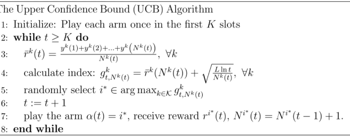
2.1 pseudocode for the UCB algorithm . . . 46

2.2 pseudocode for the UCB-M algorithm . . . 48

2.3 regrets of UCB and Anantharam’s policy . . . 53

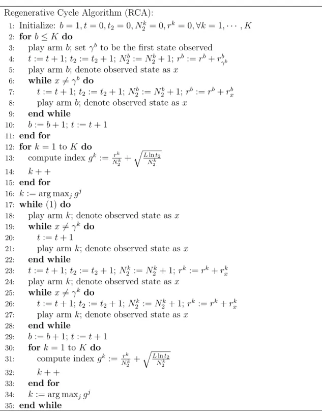
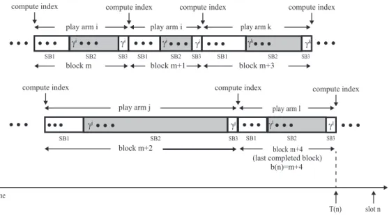
3.1 example realization of RCA . . . 60

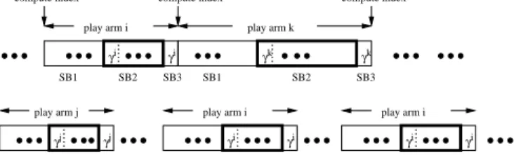
3.2 the block structure of RCA . . . 60

3.3 pseudocode of RCA . . . 62

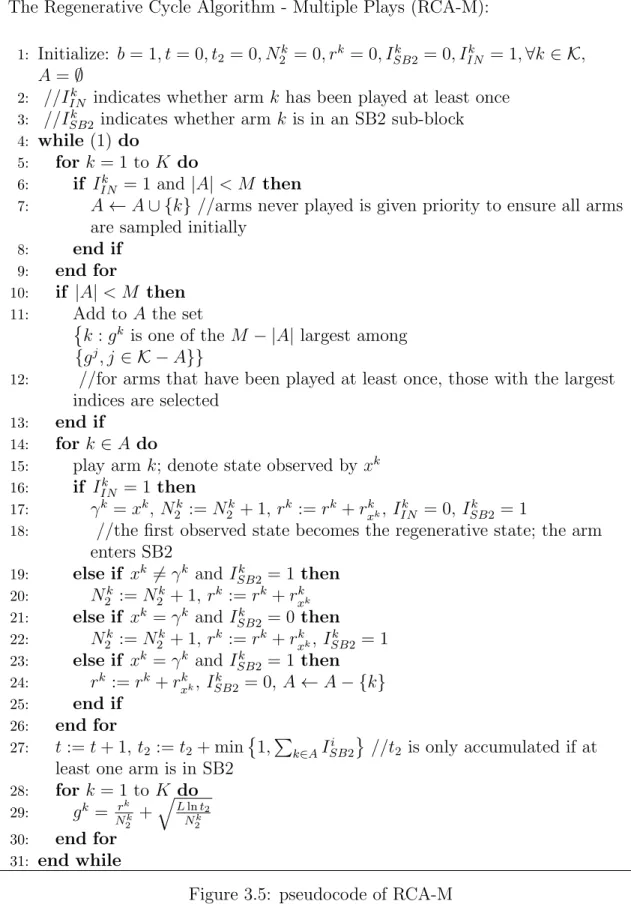
3.4 example realization of RCA-M with M = 2 for a period of n slots . 65 3.5 pseudocode of RCA-M . . . 66

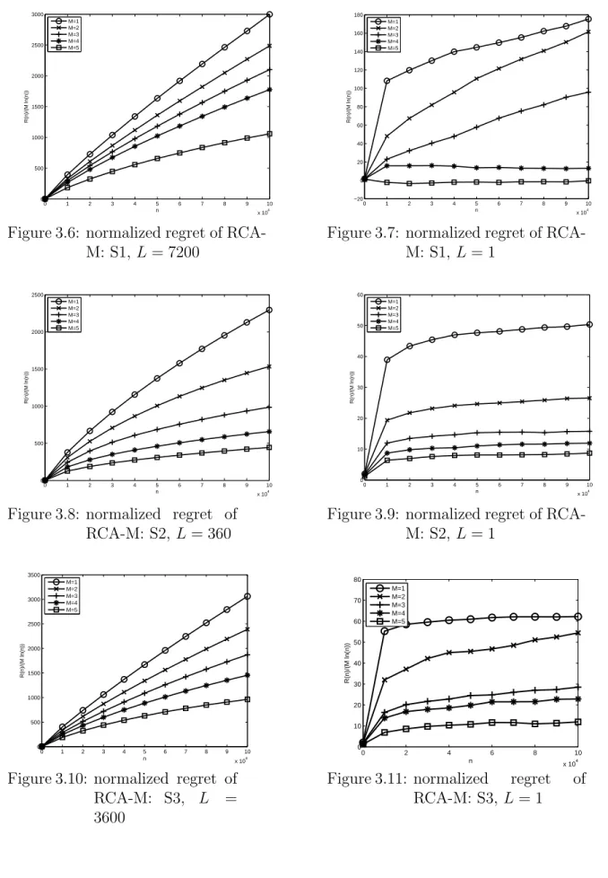
3.6 normalized regret of RCA-M: S1, L= 7200 . . . 70

(10)

3.14 regret of UCB, M = 1 . . . 71

3.15 regret of UCB, M = 1 . . . 71

3.16 regret of RCA with modified index . . . 71

4.1 pseudocode for the Average Reward with Estimated Probabilities (AREP) . . . 89

4.2 Partition of C on Ψ based on P and τtr. Gl is a set with a single information state and Gl0 is a set with infinitely many information states. . . 94

4.3 -extensions of the sets in Gτtr on the belief space. . . 95

5.1 policy Pk τ . . . 116

5.2 Guha’s policy . . . 116

5.3 procedure for the balanced choice of λ. . . 116

5.4 pseudocode for the 1-threshold policy . . . 117

5.5 pseudocode for the Adaptive Balance Algorithm (ABA) . . . 123

6.1 pseudocode of DRCA . . . 137

6.2 regret of DRCA with 2 users . . . 143

7.1 pseudocode of Exp3 . . . 160

7.2 pseudocode of RLOF . . . 166

7.3 pseudocode of DLOE . . . 179

7.4 pseudocode of DLC . . . 195

8.1 acceptance region of bundle (x1, . . . , xm) forUB(x, θ) =h(a(x−θ)++ b(θ−x)+_{) . . . .} ₂₁₁

8.2 acceptance region of bundle (x1, . . . , xm) forUB(x, θ) = −a(θ−x)+−x212 8.3 pseudocode of TLVO . . . 214

(11)

8.4 bundles of m contracts offered in exploration steps l = 1,2, . . . , l0 in an exploration phase . . . 225 8.5 pseudocode of the exploration phase of TLFO . . . 226

(12)

LIST OF TABLES

Table

2.1 frequently used expressions . . . 45

2.2 parameters of the arms for θ = [7,5,3,1,0.5] . . . 53

3.1 frequently used expressions . . . 61

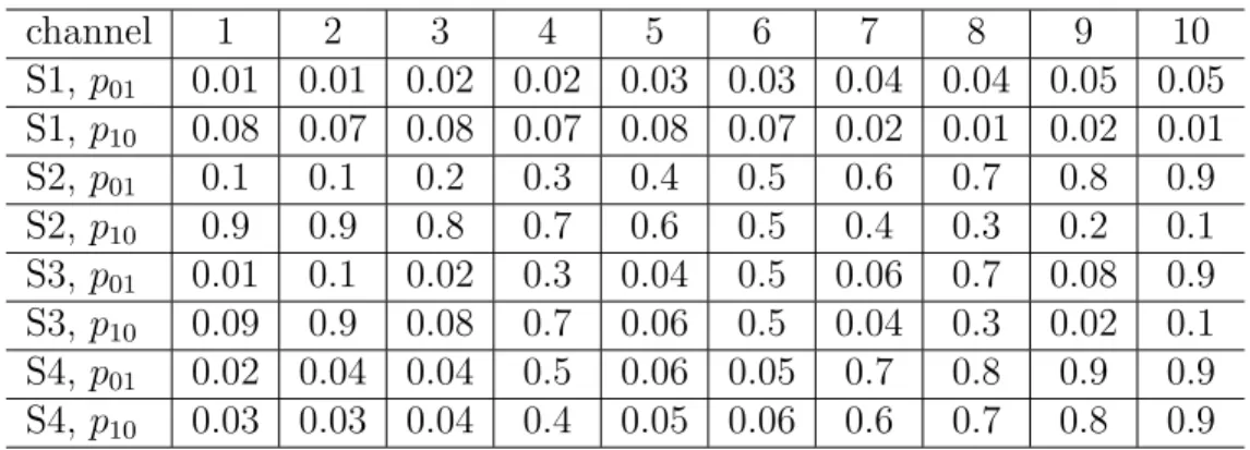
3.2 transition probabilities of all channels . . . 69

(13)

LIST OF APPENDICES

Appendix

A. Results from the Theory of Large Deviations . . . 234

B. Proof of Lemma II.2 . . . 238

C. Proof of Lemma III.1 . . . 243

D. Proof of Theorem III.2 . . . 246

E. Proof of Theorem III.3 . . . 250

F. Proof of Lemma IV.13 . . . 258

G. Proof of Lemma IV.17 . . . 261

H. Proof of Lemma IV.18 . . . 264

I. Proof of Lemma IV.19 . . . 268

J. Proof of Lemma IV.20 . . . 269

K. Proof of Lemma VI.1 . . . 271

L. Proof of Lemma VI.3 . . . 273

(14)

ABSTRACT

Online Learning in Bandit Problems by

Cem Tekin

Chair: Mingyan Liu

In a bandit problem there is a set of arms, each of which when played by an agent yields some reward depending on its internal state which evolves stochastically over time. In this thesis we consider bandit problems in an online framework which involves sequential decision-making under uncertainty. Within the context of this class of prob-lems, agents who are initially unaware of the stochastic evolution of the environment (arms), aim to maximize a common objective based on the history of actions and ob-servations. The classical difficulty in a bandit problem is the exploration-exploitation dilemma, which necessitates a careful algorithm design to balance information gath-ering and best use of available information to achieve optimal performance. The motivation to study bandit problems comes from its diverse applications including cognitive radio networks, opportunistic spectrum access, network routing, web ad-vertising, clinical trials, contract design and many others. Since the characteristics of agents for each one of these applications are different, our goal is to provide an agent-centric approach in designing online learning algorithms for bandit problems.

When there is a single agent, different from the classical work on bandit problems which assumes IID arms, we develop learning algorithms for Markovian arms by

(15)

considering the computational complexity. Depending on the computational power of the agent, we show that different performance levels ranging from optimality in weak regret, to strong optimality can be achieved.

Apart from classical single-agent bandits, we also consider the novel area of multi-agent bandits which has informational decentralization and communication aspects not present in single-agent bandits. For this setting, we develop distributed online learning algorithms that are optimal in terms of weak regret depending on commu-nication and computation constraints.

(16)

CHAPTER I

Introduction

1.1

Description and Applications of Bandit Problems

The bandit problem is one of the classical examples of sequential decision making under uncertainty. There is a set of discrete time stochastic processes (also referred to as arms) with unknown statistics. At any discrete time step (t = 1,2, . . .), each arm is in one of a set of states where the state process is generally assumed to be an independent and identically distributed (IID) or Markovian process. There is a set of players (agents), each selecting an arm at each time step in order to get a reward depending on the state of the selected arm. The evolution of the state of an arm may be independent of the actions of the agents or it may depend on the actions of the agents who select that arm. An agent has partial information about the system, which means that at any time step t, the agent only knows a subset of what has happened up to time t, and is limited to base its decision at time t on its partial information.

As an example, at any time step t, an agent can only observe the state of the arm it selects but not the states of the other arms. Another example is a multi-agent system in which an agent cannot observe the actions of other agents, or can only observe the actions of agents that are located close to it.

(17)

various performance objectives by taking into consideration a series of constraints inherent in the system.

Constraints inherent in the system include decentralization, limited computational power of the agents, and strategic behavior. We study various degrees of decentral-ization ranging from no communication between the agents at any time to full com-munication between the agents, in which each agent knows all the past observations and actions of all the agents at any time. Computational power of the agents bounds the computational complexity of the algorithms we design for the agents. Strategic behavior makes an agent act in a selfish way to maximize its own total reward, which may not coincide with the actions that will maximize the collective performance of all agents.

While the details are different under different constraints, general idea is to balance exploration and exploitation, i.e., reducing the uncertainty about the statistics of the underlying stochastic process and state of the system by playing the infrequently se-lected arms, and exploiting the best arms sese-lected according to an optimality criterion based on estimates of the statistics and the state of the system.

Our motivation to study bandit problems comes from its strength in modeling many important sequential decision making scenarios such as those occur in commu-nication networks, web advertising, clinical trials and economics. Several applications of bandit problems are given below.

1.1.1 Random Access in Fading Channels

Consider a network of M decentralized agents/users and K arms/channels. Each user can be seen as a transmitter-receiver pair. Let Sk _{be the set of fading states of} channel k. At each time step channel k is in one of the fading states s ∈ Sk _which evolves according to an IID or Markovian process with statistics unknown to the users. If user i is the only one using channelk at timet with the channel in fading state s,

(18)

then it gets a certain (single-user) channel quality given by someqk(s), where without loss of generalityqk :Sk→[0,1]; for instance this could be the received SNR, packet delivery ratio or data throughput. When there are n users simultaneously using the channel, then under a collision model in each time step each user has a probability _n1 of obtaining access, which results in a channel quality/reward of

rk(s, n) = 1

nqk(s) .

Although the system is decentralized, each user knows the number of users on the channel it selects by using some signal detection method such as an energy detector or a cyclostationary feature detector. The goal of the users is to maximize the total cumulative expected reward of all users up to any finite time horizon T.

1.1.2 Cognitive Radio Code Division Multiple Access

Consider a network ofM decentralized (secondary) agents/users andK (licensed) arms/channels. Primary users who are the licensed users of the channels have the priority in using the channels. Let s ∈ {0,1} denote the primary user activity on channel k: s= 1 if there is no primary user on channel (or channel is available) and

s = 0 otherwise. A secondary user is only allowed to access the channel if s = 1. The primary user activity on channel k is modeled as a two-state Markov chain with state transition probabilities pk

01 and pk10 unknown to the users. Multiple secondary users share access to the channel using code division multiple access (CDMA). When channel k is not occupied by a primary user, the rate a secondary user igets can be modeled as (see, e.g. Tekin et al.(2012)),

log 1 +γ h k iiPik No+P_j6=ih k jiPjk ! ,

(19)

where hk

ji is the channel gain between the transmitter of user j and the receiver of user i, Pk

j is the transmit power of user j on channel k, No is the noise power, and

γ > 0 is the spreading gain. If we assume the rate function to be user-independent, i.e.,hk

ii= ˆhk,∀i∈ M,hkji = ˜hk,∀i6=j ∈ M,Pik =Pk,∀i∈ M, which is a reasonable approximation in a homogeneous environment, then we obtain

rk(s, n) = slog 1 +γ ˆ hk_Pk i No+ (n−1)˜hkPk ! .

The goal of the users is to maximize the total cumulative reward by minimizing the number of wasted time slots due to primary user activity, and minimizing the congestion due to multiple secondary users using the same channel.

1.1.3 Adaptive Clinical Trials

Clinical trials are one of the main motivations in development of bandit problems. In an adaptive clinical trial several treatments are applied to patients in a sequential manner, and patients are dynamically allocated to the best treatment. Consider K

treatments/arms which represent K different doses of a drug. Consider a population P for which this drug is going to be used. P may be the citizens of a country, or it can be the set of people with a specific health condition such as diabetes. The effectiveness of a dose can vary from patient to patient in population P depending on genetic factors, lifestyle, etc. Let S be the space of genetic factors, lifestyle preferences, etc., that determines the effectiveness of the drug. Then, for any s∈ S, the effectiveness of dose K is given byrk₍_s_{). Let} _F _{be the distribution of population} _P _over _S_{. Then} the effectiveness of dose k is

µk =

Z

(20)

F may be unknown since S can be very large, and not all the people in population P is categorized based on the factors that determine the effectiveness of the drug. S

may be even unknown since all factors that determine the drug efficiency may not be discovered yet. Consider a subset PT of population P, which will participate in a clinical trial. We assume that PT represents the characteristics of P well, i.e., the distribution of PT over S is also (approximately) F. Patients in PT are randomly ordered, and sequentially treated. At each time step one of the doses is given to a patient, then its efficiency is observed at the end of that time step. The goal of the clinical trial is to find the most effective dose for population P while minimizing the number of patients in PT that are given less effective doses.

1.1.4 Web Advertising

A significant portion of the revenues of Internet search engines such as Google, Yahoo! and Microsoft Bing come from advertisements shown to a user based on its search query. Usually, the search engine shows a list of results based on the query with the top result being an advertisement related to that query. If the user clicks on the ad, then the search engine receives a payment from the advertiser. Assume that the search engine has K different ads/arms for a specific query. Let P denote the set of internet users that use the search engine in a specific country. The search engine does not know the percentage of users in P which will click on ad k if it is shown for query q. Moreover, this percentage can change over time, due to changing trends, consumer behavior, etc. The goal of the search engine is to display ads in a way that will maximize the number of clicks, hence the revenue. The search engine can maximize the number of clicked ads by balancing exploration of potentially relevant ads and exploitation of estimated best ads.

(21)

1.1.5 Online Contract Design

Consider a seller, who offers a set of m contracts xt = (x1, x2, . . . , xm)t ∈ X at each time step t to sequentially arriving buyers, where X is the set of feasible offers. Without loss of generality, we assume that X includes all offers x= (x1, x2, . . . , xm) for which xi ∈ (0,1] and xi ≤ xi+1 for all i. Let θt be the type of buyer arriving at time t, which is sampled from a distribution F that is unknown to the seller. Based on its type, the buyer will accept a single contract inxt or it may reject all contracts inxt. The preference of a typeθbuyer is given in terms of its utility functionUB(x, θ) which is the payoff the buyer receives when it accepts contract x. In this problem, the seller knows UB(x, θ), but it does not know the buyer’s type θ or its distribution

F. At timet, the seller receives a payoffUs(xt) =us(x) if the buyer accepts contract

x∈ xt. For a set of contracts x, E[Us(x)] depends on UB(x, θ) and the distribution of buyers type F. The goal of the seller is to maximize its expected payoff up to T

which is

T

X

t=1

E[Us(xt)].

This contract design problem is equivalent to the following bandit problem: Each

x = (x1, x2, . . . , xm) ∈ X is an arm. At each time step the seller selects one of the arms x∈ X, and receives a random reward Us(x). Let

x∗ = arg max

x∈X

E[Us(x)],

be the arm (or set of arms) that gives the highest expected reward to the seller. Then, the goal of the seller can be restated as minimizing the regret which is given by

T E[Us(x∗)]− T

X

t=1

(22)

Note that online contract design is different from the previous applications in the following ways. Firstly, X is an uncountable set. Therefore, exploring each arm separately to assess its average reward is not feasible. Secondly, dimension of X increases with the number of simultaneous offers m. This implies that the problem has a combinatorial structure. Despite these difficulties, this problem is tractable because the arms are correlated. The expected reward from each arm depends on the buyer’s type distribution F.

Due to its different structure, we formulate this problem separately in Chapter VIII, while the formulation for all other bandit problems we consider is given in the next section.

1.2

Problem Definition and Preliminaries

In a bandit problem there are K arms indexed by the set K = {1,2, . . . , K}. There is a set of agents who select a subset of the arms in a sequential manner. We assume a discrete time model,t= 1,2, . . ., where state transitions and decisions occur at the beginning of each time slot. Let Sk _{be the state space of arm} _k _{which can} be either finite or infinite. In the centralized setting, there is an agent who selects

M ≤ K of the arms at each time step. In the decentralized setting there are M

agents indexed by the set M ={1,2, . . . , M}, each of which selects a single arm at each time step. An agent has a partial observation of the state of the system which consists of observations of the rewards of the states of the arms that the agent has selected up to the current time.

Upon selecting an arm, an agent receives a reward depending on the state of that arm. The reward of armk at timet is denoted byrk₍_t_{). This reward depends on the} state of the arm, as well as the selections of the other agents.

Initially, an agent does not have any information about how the rewards of the arms are generated. The goal of the agents is to maximize a global objective. To

(23)

do this, they should learn how the rewards of the arms are generated and which arms yield highest rewards based on the current state of the system. In the following subsections we propose models for evolution of the arms, interaction between the agents, and give the definitions of performance metrics.

1.2.1 Arm Evolution Models

We consider the following stochastic models for arm state evolution.

Definition I.1. IID model: At each time step the kth arm is in a state s which is drawn from a distributionPk _over_Sk_{, independently from other time steps and other} arms.

Although, IID model is a simple yet elegant mathematical model for which sharp results can be derived, realistic modeling of many real-world applications require incorporation of temporal information. A more complicated, yet analytically tractable model is the Markovian model. In a Markovian model, the quality of an arm is reflected by its state, which evolves in a Markovian fashion. Below we give several Markovian models.

Definition I.2. Rested Markovian model: An arm has two modes,activeandpassive. An arm is active if it is selected by an agent, otherwise it is passive. In the active mode the kth arm is modeled as a discrete-time, irreducible and aperiodic Markov chain with a finite state space Sk_{. When an arm is played, transition to the next} state occurs according to the transition probability matrix Pk ₌ _pk

xy

x,y∈Sk, where pk

xy is the transition probability from state xto statey. In the passive mode the state of the arm remains frozen, i.e., it does not change. State changes of different arms are independent.

Definition I.3. Restless Markovian model: An arm has two modes, active and pas-sive. An arm is active if it is selected by an agent, otherwise it is passive. Arm k is

(24)

modeled the same way as its rested counterpart in the active mode, independent of other arms. However, in the passive mode the state of the arm changes arbitrarily.

While in the restless Markovian model, we allow a very general model for the passive mode of an arm, some of our results require a stronger assumption which requires a restless arm to be uncontrolled, i.e., the state transition of the arm is independent of the actions of agents.

Definition I.4. Uncontrolled restless Markovian model: The state evolution of an arm is independent of actions of the agents. An arm is modeled the same way as a rested arm in the active mode.

Many real-world problems can be modeled as a restless Markovian bandit. One example is a patient for which a new treatment is applied. The health condition of the patient can be modeled with a finite set of states which evolve differently when she is under the treatment and when she is not. Moreover many real-world problems are uncontrolled. For example, in a cognitive radio network, the primary user activity is independent of the secondary users’ actions.

Under the Markovian models, since each arm in the active mode is a finite state, irreducible, aperiodic Markov chain, a unique stationary distribution exists. Let

πk ={π_xk, x∈Sk}denote the stationary distribution of armk. For both the IID and the Markovian models let P = (P1, P2, . . . , PK).

1.2.2 Reward Models

In this section we list the models which describe how the agents receive rewards from the arms.

1.2.2.1 A Single-agent Reward Model

Reward the agent gets from arm k at timet only depends on the statexk_t of arm

(25)

is

rk_x ∈[0,1],

while our results will hold for any reward function that is bounded. The mean reward of arm k is given by

µk :=

Z

Sk

r_xkPk(dx),

in the IID arm evolution model, and by

µk:= X x∈Sk

rk_xπk_x,

in the Markovian arm evolution model.

1.2.2.2 Multi-agent Reward Models

In the decentralized multi-agent setting interaction between the agents plays an important role in the performance. Agents interact when they select the same arm at the same time. The interaction between agents may change their ability to collect rewards. For example, in a communication network, a transmitter-receiver pair can be regarded as an agent. If two transmitters use the same channel, due to the signal interference the receivers of both transmitters may fail to correctly decode the signal. As a result, communication is delayed, and the energy used in transmitting the signal is wasted. Below we list different interaction models.

Definition I.5. Collision model: If more than one agent selects the same arm at the same time step, all of the agents who selected the same arm gets zero reward. A collision only affects the ability of an agent to collect the reward. It does not affect the ability of an agent to observe the reward.

(26)

The communication network scenario described above fits to the collision model. Definition I.6. Random sharing model: If more than one agent selects the same arm at the same time step, they share the reward in an arbitrary way. Random sharing only affects the ability of an agent to collect the reward. It does not affect the ability of an agent to observe the reward.

An example of the random sharing model is the random access scheme in a com-munication network. Upon selecting a channel, an agent generates an exponential backoff time (which is negligible compared to the transmission/time slot length). The agent waits, and senses the channel again at the end of the backoff time. If sensed idle (there is no other agent transmitting on the channel), the agent transmits on that channel. Otherwise it does not transmit and selects another channel in the next time slot. Note that in both of the multi-agent models defined above, the mean reward of arm k is the same as the mean reward in the single-agent model.

Definition I.7. General symmetric interaction model: An agent who selects arm k

at time t gets reward rk(xtk, ntk), where xtk is the state of arm k at time t and ntk is the number of agents on arm k at timet. Without loss of generality we assume that

rk :Sk× M → [0,1],

while our results will also hold for any bounded function.

Let (k, n) denote an arm-activity pair where k denotes the arm’s index, and n

denotes the number of agents selecting that arm. In the general symmetric interaction model, the mean reward of an arm depends on the agents’ selections therefore it is not only a function of the stochastic evolution of the states of that arm. However, mean reward of the pair (k, n) does not depend on the agents’ selection and can be written only in terms of the stochastic model of the states of arm k. For the general

(27)

symmetric interaction model with the IID arm evolution model the mean reward of arm-activity pair (k, n) is given by

µk,n :=

Z

Sk

rk(x, n)Pk(dx),

and with the Markovian arm evolution model it is given by

µk,n :=

X

x∈Sk

rk(x, n)πxk.

It can be the case that the reward an agent gets decreases as more agents select the same arm with it. In this case the interaction model is called theinterference model. An example of this is the random access in fading channels scheme given in Section 1.1.

Definition I.8. Agent-specific interaction model: An agent who selects armk at time

tgets rewardri_k(xt_k, nt_k), wherext_kis the state of armkat timetand nt_k is the number of agents on arm k at time t. Without loss of generality we assume that

r_ki :Sk× M → [0,1],

while our results will also hold for any bounded function.

For the agent-specific interaction model with the IID arm evolution model the mean reward of arm-activity pair (k, n) for agent i is given by

µi_k,n :=

Z

Sk

(28)

and with the Markovian arm evolution model it is given by

µi_k,n := X x∈Sk

r_ki(x, n)π_xk.

In the agent-specific interaction model, the reward an agent gets not only depends on the state and the actions of other agents, but it is also depends on the type of the agent itself. An example of this is the cognitive radio CDMA scheme given in Section 1.1.

1.2.3 Performance Models

In this thesis, unless otherwise stated, we assume that the agents are cooperative. Their goal is to maximize a performance objective such as the sum of the expected total rewards of all agents. Therefore, our goal is to design online learning algorithms for the agents to reach their goal. The loss in performance can be due to the decen-tralization of agents, the unknown stochastic arm rewards and partial observability of the state of the system.

We compare the performance of the learning algorithms with performance of poli-cies which are given hindsight information or information about the distribution of arm states, or with centralized policies in which agents can agree at each time step on which set of arms to select. The performance loss of an algorithm with respect to such a policy is called the regret of the algorithm. We can extend the definition of regret to capture computation, switching and communication costs. Although these costs are not directly related with the stochastic evolution of the states and the agents’ ability to collect rewards, they reduce the benefit of the collected reward to an agent. For example when an agent needs to solve an NP-hard problem to find which arms to select in the next time step, we can associate a cost Ccmp with such a computationally hard operation. Moreover, we can add switching cost Cswc, which

(29)

is incurred when an agent changes the arm it selects, and communication cost Ccom, which is incurred when an agent communicates with other agents to share its infor-mation about the system or receive inforinfor-mation from other agents. For example, in opportunistic spectrum access, switching cost models the energy and time spent in changing the operating frequency of a radio, while communication cost captures the energy and other resources used to transmit signals between the agents. Without loss of generality, we assume that computation, switching and communication costs are agent-independent, i.e., the cost of each of these is the same for all agents.

Online learning algorithms used by the agents choose the arms based on the past actions and observations. In the single-agent model for an agent using algorithm α, the set of arms selected at time t is denoted by α(t) = {α1(t), . . . , αM(t)}. In the multi-agent model, when agent i uses algorithm αi, the arm selected by agent i at time t is denoted by αi(t), and the set of arms selected by all M agents at time t is denoted by α(t) = {α1(t), . . . , αM(t)}. Let EαP denote the expectation operator when algorithmα is used, and the set of arm state distributions is P. Whenever the definition of expectation is clear from the context, we will drop superscript and the subscript and simply use E for the expectation operator.

Below we give definitions of various performance measures used in single-agent and multi-agent models.

1.2.4 Single-agent Performance Models

In a single-agent bandit, there is no decentralization of information. Therefore, the contribution to regret comes from unknown stochastic arm rewards and partially observable states.

Let σ = {σ1, σ2, . . . , σK} be a permutation of arms such that the mean arm rewards are ordered in a non-increasing way, i.e., µσ1 _≥ _µσ2 _≥ _{. . .} _≥ _µσK_{. Let} _rk₍_t₎

(30)

Below is the definition of weak regret for a single agent (stochastic) bandit. Definition I.9. Weak regret in the single-agent model: For an agent using algorithm

α, selecting M ≤K arms at each time step, the weak regret up to time T is

Rα(T) := T M X k=1 µσk ₋_EP α   T X t=1 X k∈α(t) rk(t)  ,

where α(t) is the set of arms selected by the agent at timet.

When we add computation and switching costs, the weak regret becomes

Rα(T) :=T M X k=1 µσk ₋_EP α   T X t=1 X k∈α(t) rk(t)−Ccmpmcmp(T)−Cswcmswc(T)  , (1.1)

where mcmp(T) denotes the number of NP-hard computations by the agent by time

T, and mswc(T) denotes the number of times the agent switched arms by time T. Under the IID model, weak regret compares the performance of the algorithm with respect to the optimal policy given full information about the stochastic dynamics. This is also true under the rested Markovian model with a large time horizonT. This is because under these models the optimal policy is a static one. However, under the restless Markovian model, the optimal policy is no longer a static one. In general, the optimal policy dynamically switches between the arms based on the perceived state of the system by the agent. The regret with respect to such an optimal policy is calledstrong regret.

Definition I.10. Strong regret in the uncontrolled restless single-agent model: Let Γ be the set of admissible policies which can be computed using the stochastic dynamics of the arms. Those are the policies for which the action of agent at any time depends on the set of transition probabilities P = {P1, P2, . . . , PK}, initial belief about the state of the system ψ0, and past observations and actions. For an agent using a

(31)

learning algorithm α, selecting M ≤K arms at each time step, the strong regret by time T is Rα(T) := sup γ0_∈_Γ  E_ψP 0,γ0   T X t=1 X k∈γ0_(t) rk(t)    −E_ψP 0,α   T X t=1 X k∈α(t) rk(t)  .

In the definition of strong regret, we compare the performance of the learning algo-rithmαwith the optimal policy computed without taking computation and switching costs into consideration. Note that whenP is known, the optimal policy is computed once, at the beginning, and the agent plays according to that policy. Therefore the optimal policy given P does not depend on the cost of computation. However, a policy which is optimal when there are no switching costs may not be optimal when there are switching costs. When we introduce the switching cost Cswc, the strong regret becomes Rα(T) := sup γ0_∈_Γ  E_ψP₀_,γ0   T X t=1 X k∈γ0_(t) rk(t)−Cswcmswc(T)     −E_ψP₀_,α   T X t=1 X k∈α(t) rk(t)−Cswcmswc(T)−Ccmpmcmp(T)  . (1.2)

Note that the strong regret is a stronger performance measure than infinite horizon average reward. Firstly, it holds for all finiteT. Secondly, even if two algorithms have the same average reward, the difference between their asymptotic regret (as T → ∞) can be unbounded. In fact, strong regret specifies how fast the algorithm converges to the optimal average reward. An alternative performance measure is to compare the average reward of the algorithm with the average reward of the optimal policy with known stochastic dynamics. This performance measure is called approximate optimality.

(32)

average reward of the optimal policy given the stochastic dynamics. The learning algorithm α for the agent is approximately optimal if

lim inf T→∞E P α " PT t=1 P k∈α(t)r k₍_t₎ T # ≥OP T.

Similar to the strong regret model, we can incorporate computation and switchings costs to the approximate optimality criterion. Note that any algorithm with sublinear number of computations and switchings in time will have the same average reward as the optimal policy computed without computational and switching costs.

1.2.5 Multi-agent Performance Models

For the multi-agent model we only consider weak regret. For definition of the weak regret we need to consider the interaction between the agents. Firstly, we define the regret for the collision model given in Definition I.5. For all agent interaction models except the agent-dependent interaction model, we assume that agents cannot communicate with each other. Therefore, we do not include to cost of communication for these models.

Definition I.12. Weak regret in the collision model: With M decentralized agents, under the agent interaction model given in Definition I.5, when agentiuses algorithm

αi to select a single arm at each time step, the weak regret up to time T is

Rα(T) := T M X k=1 µσk ₋_EP α " _T X t=1 M X i=1 rαi(t)₍_t₎_I₍_nt αi(t) = 1) # ,

where αi(t) is the arm selected by agent i at time t, and I(nt_α_i_(t) = 1), which is the indicator function of the event {nt

(33)

is collected only when agent iis the only agent on that arm, or equivalently Rα(T) = T M X k=1 µσk ₋_EP α " _T X t=1 K X k=1 rk(t)I(nt_k = 1) # .

Definition I.13. Weak regret in the random sharing model: With M decentralized agents, under the agent interaction model given in Definition I.6, when agent i uses algorithm αi to select a single arm at each time step, the weak regret up to timeT is

Rα(T) :=T M X k=1 µσk ₋_EP α " _T X t=1 K X k=1 rk(t)I(nt_k≥1) # .

Even though we will not analyze the random sharing model directly, for the al-gorithms we propose, the upper bounds on regret we prove in the collision model will also hold for the random sharing model. This is because the observations of the agents remains the same (since we assume that collision does not affect an agents ability to observe the reward, but only effects its ability to collect the reward), while at each time step the collected reward in the random sharing model is greater than or equal to the collected reward in the collision model.

Note that for all the definitions of the weak regret above, we compare the algo-rithms performance with respect to the strategy that always selects theM best arms, which is an orthogonal configuration, i.e., all agents select different arms. The com-putation and switching costs can be added to the weak regret in a similar way with the single agent model. For example, the weak regret of the collision model becomes

Rα(T) := T M X k=1 µσk₋_EP α " _T X t=1 K X k=1 rk(t)I(nt_k = 1)−Ccmp M X i=1 mi_cmp(T) −Cswc M X i=1 mi_swc(T) # , (1.3) where mi

(34)

mi

swc(T) is the number of switchings by agent i by timeT.

For the general symmetric interaction model given in Definition I.7, we need to take into account the fact that there may be more than one agent on each arm in the optimal allocation. In the general symmetric interaction model, let rk,n(t) be the random variable which denotes the reward of arm-activity pair (k, n) at time t. It is important not to confuse this random variable withrk(x, n) which denotes the reward from statex of arm k when there are n agents on it.

Definition I.14. Weak regret in the general symmetric interaction model: Given

µk,n,∀k ∈ K, n∈ M, the optimal allocation of arms to agents is the set of allocations

A∗ := arg max a∈A M X i=1 µai,nai(a),

wherea= (a1, a2, . . . , aM)∈ Ais the vector of arms chosen by the agents 1,2, . . . , M respectively, nk(a), k ∈ K is the number of agents on arm k under vector a, and A :={a : ai ∈ K,∀i ∈ M} is the set of possible arm selections by the agents. Let N :={n= (n1, n2, . . . , nK) :nk ≥0, n1+n2 +. . .+nK =M} be the set of possible number of agents on (agents selecting) each arm, where nk is the number of agents on arm k. An equivalent definition of the optimal allocation in terms of elements of N is N∗ := arg max n∈N K X k=1 nkµk,nk.

Letv∗ be the value of the optimal allocation. Then the weak regret by timeT is

Rα(T) :=T v∗−E_αP " _T X t=1 M X i=1 r_α_i_(t),nt αi(t)(t) # .

It turns out that in the general symmetric interaction model, an agent should form an estimate of the best combination of agents and arms. Forming such an estimate

(35)

is a combinatorial optimization problem which is NP-hard in general. Thus, adding computation and switching costs, the weak regret becomes

Rα(T) :=T v∗−E_αP " _T X t=1 M X i=1 r_α_i_(t),nt αi(t)(t)−Ccmp M X i=1 mi_cmp(T) −Cswc M X i=1 mi_swc(T) # . (1.4)

A generalization of the general symmetric interaction model is the agent-specific in-teraction model which is given in Definition I.8. In this model, let ri_k,n(t) be the random variable which denotes the reward of arm-activity pair (k, n) to agent i at time t. Since the observations of an agent in this case does not provide any informa-tion about the rewards of other agents, agents should share their percepinforma-tion of the arm rewards with other agents in order to cooperatively achieve some performance objective. We assume that whenever an agent communicates with any other agent, it incurs cost Ccom.

Definition I.15. Weak regret in the agent-specific interaction model: Givenµi_k,n,∀k ∈ K, i, n∈ M, the set of optimal allocations is

A∗ = arg max a∈A M X i=1 µi_a_i_,n ai(a),

where a = (a1, a2, . . . , aM) ∈ A is the vector of arms selected by agents 1,2, . . . , M respectively, and A=KM _{is the set of possible arm selections by the agents. Let} _v∗

be the value of the optimal allocation. Then the weak regret by time T is

Rα(T) :=T v∗−E_αP " _T X t=1 M X i=1 ri_α i(t),nt_αi₍_t₎(t) # .

(36)

re-gret becomes Rα(T) :=T v∗−E_αP " _T X t=1 M X i=1 r_αi i(t),nt_αi₍_t₎(t)−Ccmp M X i=1 mi_cmp(T) −Cswc M X i=1 mi_swc(T)−Ccom M X i=1 mi_com(T) # . (1.5) 1.2.6 Degree of Decentralization

In this section we define various degrees of decentralization that may be possible in a multi-agent system. These settings are ordered according to increasing feedback and communication among the agents. Let ri

k(t) denote the reward agent i receives from arm k at time t.

Model I.16. No feedback. Under this model, upon selecting armkat timet, agent

i only observes the reward ri_k(t), but not the number of other agents selecting arm k

(nt_k) or state of arm k (xt_k).

For example, in a dynamic spectrum access problem where arms are channels, Model I.16 applies to systems of relatively simple and primitive radios that are not equipped with threshold or feature detectors.

Model I.17. Binary feedback. Under this model, upon selecting arm k at time

t, agent i observes the reward ri_k(t). At the end of the time slot t, agent i receives a binary feedback z ∈ {0,1} where z = 0 means that agent i is the only agent who selected armk at time t, and z = 1 means that there is at least one other agent who also selected arm k at time t.

Similar to the previous example, in a dynamic spectrum access problem, agents who are equipped with a threshold detector can infer if there are other agents who used the same channel with them.

(37)

Model I.18. Partial feedback. Under this model, upon selecting arm k at time

t, agent iobserves the reward ri

k(t) and acquires the value ntk. Moreover, each agent knows the total number of agents M.

Again, Model I.18 applies to a system of more advanced radios, those that are equipped with a threshold or feature detector. Based on the interference received, a user/agent can assess the simultaneous number of users in the same channel. The same can be achieved by each radio broadcasting its presence upon entering the network, and upon selecting a channel.

Model I.19. Partial feedback with synchronization. Under this model, upon selecting armk at timet, agentiobserves the reward ri

k(t) and acquires the valuentk. Each agent knows the total number of agentsM. Moreover, the agents can coordinate and pre-determine a joint allocation rule during initialization.

As an example, Model I.19 applies to a system of more advanced radios as in the previous model. Moreover, each radio is equipped with sufficient memory to keep an array of exploration sequences based on its identity, i.e, a sequence of channels that should be selected consecutively.

Model I.20. Costly communication. In this model, agents can communicate with each other, but communication incurs some cost Ccom >0. Upon selecting arm k at time t, agent i observes the reward ri_k(t) but nothing more.

In Model I.20, we generally assume that the agents can exchange messages over a common control channel. However, if arms are channels as in the dynamic spectrum access problem, agents can communicate over the arms. A common control channel is not needed in this case.

(38)

1.3

Literature Review

In this section we review the literature on bandit problems. We classify the bandit problems according to the number and reward generation process of the arms, corre-lation between the reward processes of the arms, and the number of agents. We also mention the bandit optimization problems, in which the goal is find computationally efficient methods to calculate the optimal policy. These problems do not involve any learning.

1.3.1 Classical Single-agent Models

The single-agent bandit problem is investigated by many researchers over the past decades. Motivated by clinical trials this problem is first studied inThompson(1933), and the seminal work Robbins (1952) set the foundations of the bandit problem. In the classical single-agent models, there is a finite set of independent arms.

Most of the existing literature assumes an IID model for the reward process of each arm. Below we discuss accomplishments in the IID model. Since the optimal policy is a static policy in the IID model, weak regret which is given in Definition I.9 compares the performance of the learning algorithm with respect to the optimal policy. Therefore for the IID model, weak regret is the same as strong regret which is given in Definition I.10. Since they are equivalent we simply call it the regret.

In Lai and Robbins (1985) the problem where there is a single agent that plays one arm at each time step is considered, assuming an IID reward process for each arm whose probability density function (pdf) is unknown to the agent, but lies in a known parametrized family of pdfs. Under some regularity conditions such as the denseness of the parameter space and continuity of the Kullback-Leibler divergence between two pdfs in the parametrized family of pdfs, the authors provide an asymptotic lower bound on the regret of any uniformly good policy. This lower bound is logarithmic in time which indicates that at least logarithmic number of samples should be taken

(39)

from each arm to decide on the best arm with a high probability. They define a policy to be asymptotically optimal if it achieves this lower bound, and then construct such a policy. This result is extended in Anantharam et al. (1987a) to single agent and multiple plays, in which the agent selects multiple arms at each time step. The policies proposed in these two papers are index policies, which assign an index to each arm based on the observations from that arm only, and select the arm with the highest index at each time step. However, complexity of deciding on which arm to select increases linearly in time both inRobbins (1952) andAnantharam et al.(1987a) which makes the learning policies computationally infeasible. This problem is addressed in Agrawal (1995a) where sample mean based index policies are constructed. The complexity of a sample mean based policy does not depend on time since the decision at each time step only depends on the average of the rewards in the previous time steps, not on the reward sequence itself. The policies proposed in Agrawal (1995a) are order optimal, i.e., they achieve the logarithmic growth of regret in time, which is shown to be the best possible rate of growth. However, they are not in general optimal because the constant term which multiplies the logarithmic expression in time is not the best possible term.

In all the papers mentioned above, the limiting assumption is that there is a known single parameter family of pdfs for arm reward processes in which the correct pdf resides. Such an assumption virtually reduces the arm quality estimation problem into a parameter estimation problem. This assumption is relaxed inAuer et al.(2002), which requires that the reward of an arm is drawn from an unknown distribution with a bounded support. Under this condition, the authors propose an index policy called

the upper confidence bound (UCB1) similar to the one inAgrawal (1995a) which only uses the sample means of the reward sequences. They prove order-optimal regret bounds that hold uniformly over time, not just asymptotically.

(40)

regret bound that has a smaller constant than the regret bound of UCB1 is proposed. In Garivier and Capp´e (2011), the authors propose an index policy, KL-UCB, which is uniformly better than UCB1. Moreover, this policy is shown to be asymptotically optimal for Bernoulli arm rewards. Authors inAudibert et al.(2009) consider the same problem withAuer et al.(2002), but in addition take into account empirical variance of the arm rewards for arm selection. They provide a logarithmic upper bound on regret with better constants under the condition that the suboptimal arms have low reward variance. In addition, they derive probabilistic bounds on the variance of the regret by studying its tail distribution.

In the papers that are mentioned above, the uniform regret bounds hold for bounded reward distributions. Online learning in bandit problems is extended to heavy-tailed reward distributions in Liu and Zhao (2011) using deterministic explo-ration and exploitation sequences. Specifically, when the reward distributions have central moments up to any order, logarithmic regret uniform in time is achievable. It is also shown that even if the reward distributions have central moments up to a finite order p, sublinear regret uniform in time, in the orderO(T1/p_{), is achievable.}

Another part of the literature is concerned with the case when the reward process for each arm is Markovian. This offers a richer framework for the analysis, especially more suitable to real-world applications including opportunistic spectrum access. Re-sults in the Markovian reward model can be divided into two groups

The first group is the rested Markovian model given in Definition I.2, in which the state of an arm evolves according to a Markov rule when it is played by the agent, and remains frozen otherwise. Similar to the IID model, it can also be shown that the weak regret and strong regret is the same for the rested Markovian model (after some finite number of time steps) and the optimal policy is a static policy that plays the arms with the highest expected rewards. A usual assumption under this model is that the reward process for each arm is modeled as a finite-state, irreducible,

(41)

aperiodic Markov chain. This problem is first addressed inAnantharam et al.(1987b) assuming a single parametrized transition probability model, where asymptotically optimal index policies with logarithmic regret is proposed. In Tekin and Liu (2010), we relax the parametric assumption on transition probabilities, and prove that a slight modification of UCB1 in Auer et al. (2002) achieves logarithmic regret uniformly in time for the rested Markovian problem. Different from Anantharam et al. (1987b) our result holds for any finite time, and our algorithm, which needs only the sample mean of the collected rewards, is computationally simpler. However, the constant that multiplies the logarithmic term is not optimal. This work constitutes Chapter II of the thesis.

The second group is the restless Markovian model in which the state of an arm evolves according to two different Markov rules depending on whether the agent played that arm or not. Clearly, the optimal policy is not necessarily a static policy, thus weak regret and strong regret are different performance measures for this model. This problem is significantly harder than the rested Markovian case, and even when the transition probabilities of the arms are known by the agent, it is PSPACE hard to approximate as shown in Papadimitriou and Tsitsiklis (1999). Because of this diffi-culty, most of the authors focus on algorithms whose performance can be evaluated in terms of the weak regret. Specifically, inTekin and Liu(2011b) we propose a learning algorithm which estimates mean rewards of the arms by exploiting the regenerative cycles of the Markov process. This algorithm is computationally simple and requires storage which is linearly increasing in the number of arms. We prove that this algo-rithm has logaalgo-rithmic weak regret for a more general restless Markovian model given in Definition I.3. This work constitutes Chapter III of the thesis. In a parallel work,

Liu et al.(2010), the idea of geometrically growing exploration and exploitation block lengths is used to prove a logarithmic weak regret bound. The difference is that the block lengths in Liu et al. (2010) is deterministic, while the block lengths in Tekin

(42)

and Liu (2011b) are random.

Since weak regret does not provide a comparison with respect to the optimal policy for the restless Markovian model, we study stronger measures of performance in Tekin and Liu (2012a) and Tekin and Liu (2011a), which forms Chapters V and IV of this thesis. Specifically, in Tekin and Liu (2012a) we consider an approxi-mately optimal, computationally efficient algorithm for a special case of the restless Markovian bandit problem which is called the feedback bandit problem. This prob-lem is studied inGuha et al. (2010) in an optimization setting rather than a learning setting. We combine learning and optimization by using a threshold variant of the op-timization policy proposed inGuha et al.(2010) in exploitation steps of the proposed learning algorithm. Because of the computational complexity result inPapadimitriou and Tsitsiklis (1999), it is not possible to achieve logarithmic strong regret with a computationally feasible algorithm for the restless Markovian model. However, the existence of a learning algorithm with logarithmic strong regret is still an interesting open problem. In Tekin and Liu (2011a) we consider this problem, and propose a learning algorithm with logarithmic strong regret uniform in time for the uncontrolled restless Markovian model given in Definition I.4. This result can be seen as a step towards optimal adaptive learning in partially observable Markov decision processes. Different from our work, in Dai et al. (2011) strong regret is considered with a policy-based approach. The authors assume that the agent is given a set of policies which includes the optimal policy. They provide an algorithm where there is a pre-determined sequence of blocks with increasing lengths, and during a block the policy with the highest sample mean reward up to date is selected. In essence, the algorithm treats each policy as a policy-arm, and keeps track of the sample mean rewards of each policy-arm. This algorithm achievesG(T)O(logT) strong regret, where G(T) can be an arbitrary slowly diverging sequence. Although this result is promising because it is computationally simple, in a general restless bandit problem the number of policies is

(43)

infinite, and the policy space is exponential in the number of arms. Moreover, most of the policies can be highly correlated but the algorithm considers them independently. Other than the bounds on regret, another interesting study is to derive proba-bly approximately correct (PAC) bounds on the number of explorations required to identify a near-optimal arm. In other words, find the expected number of exploration steps such that at the end of explorations the algorithm finds a near-optimal arm with high probability. Even-Dar et al. (2002) and Mannor and Tsitsiklis (2004) are some examples of the research in this direction.

Similar to learning in bandit problems, learning in unknown Markov decision pro-cesses (MDPs) is considered by several researchers. In a finite, irreducible MDP with bounded rewards, logarithmic regret bounds with respect to the best deterministic policy is considered in Burnetas and Katehakis (1997); Ortner (2007); Tewari and Bartlett (2008); Ortner (2008). In Burnetas and Katehakis (1997) the authors pro-pose an index-based learning algorithm, where the indices are the inflations of right-hand sides of the estimated average reward optimality equations based on Kullback-Leibler (KL) divergence. Although not computationally feasible, assuming that the support of the transition probabilities are known by the agent, they show that this algorithm achieves logarithmic regret asymptotically, and it is optimal both in terms of the order and the constant.

The same problem is also studied in Tewari and Bartlett (2008), and a learning algorithm that usesl1 distance instead of KL divergence with the same order of regret but a larger constant is proposed. Different form Burnetas and Katehakis (1997), knowledge about support of the transition probabilities is not required. A learning algorithm with logarithmic regret and reduced computation, which solves the average reward optimality equation only when a confidence interval is halved is considered in

Auer et al. (2009), and learning in an MDP with deterministic transitions is studied inOrtner (2008).

(44)

1.3.2 Classical Multi-agent Models

Unlike classical single-agent models, multi-agent bandit problems became a pop-ular area of research recently. Many practical applications involving multi-agent dy-namic resource allocation can be analyzed using the bandit framework. The properties of the multi-agents models that are not present in the single-agent models include in-formational decentralization, strategic/selfish behavior and communication between the agents. In a classical multi-agent bandit problem there is a finite set of indepen-dent arms.

Most of the relevant work in multi-agent bandit problems assumes that the best static configuration of agents on arms is such that at any time step there is at most one agent on an arm. We call such a configuration an orthogonal configuration. Multi-agent bandits with IID reward model is considered in Liu and Zhao (2010) and Anandkumar et al. (2011), and distributed learning algorithms with logarith-mic regret are proposed assuming that the best static configuration is an orthogonal configuration. Specifically, the algorithm in Liu and Zhao (2010) uses a mechanism calledtime division fair sharing, where an agent shares the best arms with the others in a predetermined order. Whereas in Anandkumar et al. (2011), the algorithm uses randomization to settle to an orthogonal configuration, which does not require pre-determined ordering, at the cost of fairness. In the long run, each agent settles down to a different arm, but the initial probability of settling to the best arm is the same for all agents.

In addition to the IID reward model, some researchers considered the restless Markovian model. In Tekin and Liu (2012d), we design a distributed learning algo-rithm with logaalgo-rithmic weak regret for the restless Markovian model. Our approach is based on a distributed implementation of the regenerative cycle algorithm we pro-posed for the single-agent bandits. This work forms Chapter VI of the thesis. Different from our work, in Liu et al. (2011) the authors propose a learning algorithm based

(45)

on deterministic exploration and exploitation blocks, which also achieves logarithmic weak regret for the restless Markovian model.

Although the assumption on optimality of orthogonal configuration is suitable for applications in communication systems such as random access or collision models, it lacks the generality for applications like code division multiple access and power con-trol in wireless systems. In a general resource sharing problem, agents may still get some reward by sharing the same resource. This motivates us to have an agent-centric approach to online resource sharing problems. Specifically, based on the character-istics of the agents including computation power, switching costs, communication ability and degree of decentralization, we propose online learning algorithms with variaous performance guarantees in Tekin and Liu (2011c, 2012b). This work consti-tutes Chapter VII of the thesis. Specifically, in Tekin and Liu (2011c) we propose a randomized algorithm with sublinear regret with respect to the optimal configuration of agents for the IID model, and in Tekin and Liu (2012b) we propose algorithms based on deterministic sequencing of exploration and exploitation with logarithmic weak regret with respect to the optimal configuration which work for both the IID and restless Markovian models.

1.3.3 Models with Correlation

Both the classical single-agent and multi-agent models consider finite number of independent arms. Therefore using the algorithms designed for these models will not result in optimal performance when the arms are correlated, i.e., the reward of an arm at time step t can depend on the reward of another arm at time stept. In these settings, learning algorithms that exploit the correlation between the arms perform better. In the literature there are many different assumptions about the correlation structure. However, we can group these into two main areas: bandits with finite number of arms with a combinatorial structure and bandits with infinite number of

(46)

arms.

Usually the classical models focus on achieving logarithmic regret in time, without considering the dependency of regret on the number of arms (which is linear in most of the cases), while models that exploit correlation between the arms also try to reduce the growth of regret with the number of arms (sublinear or logarithmic for finite number of arms). When there are infinitely many arms sublinear regret bounds (in time) can be achieved by exploiting the correlation. Unless otherwise stated, the results for the models with correlation is usually restricted to a single-agent.

When the number of arms is finite, an IID model where expected rewards of the arms are correlated through a linear function of an unknown scalar whose distribution is known by the agent is considered inMersereau et al.(2009), where the agent knows the distribution of the unknown scalar. Under some assumptions on the structure of known coefficients, they prove that a greedy algorithm that chooses the arm with the highest posterior mean reward is optimal in the infinite horizon discounted setting, and the play settles to the best arm with probability one. This is in contrast to the incomplete learning theorem stated in Brezzi and Lai (2000), which says that in the classical bandit setting, the agent needs to indeterminately switch between exploration and exploitation in order to avoid the possibility of settling down to a suboptimal arm. The authors also show that under the undiscounted setting the asymptotic weak regret of the greedy policy is finite, contrary to the unbounded

O(logT) regret results in the classical bandit problems. In Pandey et al. (2007) a model where the arms are separated into clusters, with the correlation between the arms in a cluster is described by a generative model with unknown parameters is considered. Authors propose a two stage algorithm that first chooses a cluster, and then an arm within that cluster. Numerical results show that exploiting the dependencies in a cluster reduces the regret.

(47)

with IID, rested Markovian and restless Markovian models respectively. In a com-binatorial bandit an agent chooses a set of arms. Reward the agent receives is a linear combination of the rewards of the individual arms. In addition to receiving the combination of rewards the agent observes the individual rewards generated by each selected arm. The number of arm combinations that the agent can choose from is ex-ponential in the number of arms, therefore classical bandit algorithms such as UCB1 suffers a regret exponential in the number of arms for this problem. Moreover UCB1 has to store an index for each combination, which also makes the storage exponential in the number of arms. The authors overcome this problem by proposing algorithms that update the index of each arm separately, and compute the optimal pair based on a bipartite matching. Both the storage and the regret of these algorithms are polynomials in the number of arms.

When there are infinitely many arms, the correlation is usually given by a dis-tance metric that relates the disdis-tance between the arms with the disdis-tance between their expected rewards. Examples of this line of work are given in Rusmevichientong and Tsitsiklis (2010); Bartlett et al. (2008); Dani et al. (2008); Jiang and Srikant

(2011). Specifically, linearly parameterized bandits in which the expected reward of each arm is a linear function of an r-dimensional random vector is considered in Rus-mevichientong and Tsitsiklis (2010). A similar linear optimization formulation of the bandit problem is considered in Dani et al. (2008). A high probability regret bound is considered in Bartlett et al. (2008) for the problem studied in Dani et al. (2008). InJiang and Srikant (2011) the authors propose another parametric model, in which an arm is associated with a finite dimensional attribute vector. In all of the papers mentioned above, learning algorithms with sublinear regret bounds are proposed.

In Kleinberg et al. (2008) the authors study Lipschitz bandits, where agents’ ac-tions form a metric space, and the reward function satisfies aLipschitzcondition with respect to this metric. They provide a sublinear lower bound on regret, and propose

(48)

a zoomingalgorithm which achieves regret arbitrarily close to the lower bound. In Tekin and Liu (2012c), we model an online contract selection problem as a bandit problem with uncountable number of arms and a combinatorial structure. Different from the work on bandits with infinitely many arms, we exploit the com-binatorial structure to prove a sublinear regret bound that has linear dependence on the dimension of the problem. This work forms Chapter VIII of the thesis.

Another type of bandits in which the correlation structure is exploited is con-textual bandits (bandits with side information). In a concon-textual bandit there is a predetermined unknown sequence of context arrivals. Different from the classical bandit setting, the decision of the agent is also based on the newly arrived context. The goal of the agent is to choose the best arm given the context. One of the early notable work in this area is Wang et al. (2005) in which exploitation of side infor-mation for a two-armed bandit setting is considered. Usually, the number of arms is infinite and the agent is given a similarity metric by which it can deduce the correla-tion between different context-arm pairs. Important papers under large arm sets are

Langford and Zhang (2007), which provides an epoch-greedy algorithm with sublin-ear regret, Slivkins (2009), which gives tight upper and lower bounds on the regret when the agent is provided with the similarity information, and Rosin (2011), which considers episodic context arrivals.

1.3.4 Non-stationary and Adversarial Models

In this section we review the literature on bandit problems with rewards generated either by a non-stationary process or by an adversary. In non-stationary bandits either the number of arms or arm reward distributions vary dynamically over time, while in adversarial bandits the arm rewards are generated by an adversary whose goal is to minimize the total reward of the agent. The adversary can be an obliviousadversary, which means that at the beginning it can choose a sequence of arm rewards according

(49)

to the agent’s algorithm to minimize the agent’s total reward, but once the agent starts playing it cannot adaptively change the sequence of arm rewards based on the history of play of the agent. The adversary capable of doing this is called theadaptive