Ching-pei Lee [email protected]
Dan Roth [email protected]
University of Illinois at Urbana-Champaign, 201 N. Goodwin Avenue, Urbana, IL 61801 USA
Abstract
Training machine learning models sometimes needs to be done on large amounts of data that exceed the capacity of a single machine, motivat-ing recent works on developmotivat-ing algorithms that train in a distributed fashion. This paper pro-poses an efficient box-constrained quadratic opti-mization algorithm for distributedly training lin-ear support vector machines (SVMs) with large data. Our key technical contribution is an ana-lytical solution to the problem of computing the optimal step size at each iteration, using an ef-ficient method that requires onlyO(1) commu-nication cost to ensure fast convergence. With this optimal step size, our approach is superior to other methods by possessing global linear con-vergence, or, equivalently,O(log(1/))iteration complexity for an -accurate solution, for dis-tributedly solving the non-strongly-convex linear SVM dual problem. Experiments also show that our method is significantly faster than state-of-the-art distributed linear SVM algorithms includ-ingDSVM-AVE,DisDCAandTRON.
1. Introduction
With the rapid growth of data volume, distributed machine learning gains more importance as a way to address train-ing with massive data sets that could not fit the capacity of a single machine. Linear support vector machine (SVM) (Boser et al., 1992; Vapnik, 1995) is a widely adopted model for large-scale linear classification. Given train-ing instances{(xi, yi)∈Rn× {−1,1}}li=1, linear SVM
solves the following problem:
min w∈Rn f P(w)≡1 2w Tw+C l X i=1 ξ(w,xi;yi), (1)
Proceedings of the32nd International Conference on Machine Learning, Lille, France, 2015. JMLR: W&CP volume 37. Copy-right 2015 by the author(s).
whereC >0is a specified parameter, andξis a loss func-tion. Two common choices ofξare
max(0,1−yiwTxi), andmax(0,1−yiwTxi)2, which we refer to as L1-SVM and L2-SVM, respectively. Linear SVM has been used in many applications, and its single-machine training has been studied extensively. It is well-known that instead of directly solving (1), optimizing its dual problem shown below is sometimes faster (Hsieh et al., 2008; Yuan et al., 2012), especially whenl < n, because there are fewer variables to optimize.
min α∈Rl f(α)≡ 1 2α TQα¯ −eTα subject to 0≤αi≤U, i= 1, . . . , l, (2) where e is the vector of ones, Q¯ = Q +sI, Q = Y X(Y X)T, X = [x
1, . . . ,xl]T,Y is a diagonal matrix such thatYi,i=yi,Iis the identity matrix, and
(s, U) =
(
(0, C) if L1-SVM, (1/2C,∞) if L2-SVM.
Because the main computations in batch solvers for (1) are matrix-vector products that can be naively parallelized, several works have successfully adapted these solvers to distributed environments (Agarwal et al., 2014; Zhang et al.,2012;Zhuang et al.,2015;Lin et al.,2014). How-ever, state-of-the-art single-machine dual algorithms are all sequential and cannot be easily parallelized. Moreover, in a distributed setting, because each machine only has a frac-tion of the training data, and the cost of communicafrac-tion and synchronization is relatively high, it is important to consider algorithms with low communication cost. Con-sequently, algorithms with a faster convergence rate are desirable because a smaller number of iterations implies a smaller number of communication rounds. We observe that without careful consideration of this issue, existing distributed dual solvers do not achieve satisfactory train-ing speed. However, as mentioned above, given that a dual solver might be more suitable for high-dimensional data, it
is important to develop better distributed dual linear SVM algorithms for extremely large data sets of high dimension-ality.
In this work, we propose an efficient box-constrained quadratic optimization framework for solving (2) when the training instances are distributed amongK machines, where the instances in machine k are {(xi, yi)}i∈Jk. In
our setting,Jkare disjoint index sets such that∪Kk=1Jk = {1, . . . , l}. By considering a carefully designed positive definite block-diagonal approximation of Q, at each iter-¯ ation our algorithm efficiently obtains a descent direction that ensures fast convergence for (2) with low communica-tion cost. We then conduct a line search method that only requires negligible computation cost andO(1) communica-tion to establish a global linear convergence rate. In other words, our algorithm only requiresO(log(1/))iterations to obtain an-accurate solution for (2). This convergence rate is better than that of existing distributed dual solvers for training L1-SVM, whose dual problem is not strongly convex. We also discuss the main differences between our algorithm and existing distributed algorithms for (2) and point out the key differences.
Experiments show that our algorithm is significantly faster than existing distributed solvers for (2). Our framework can be easily extended to solve other similar problems. This paper is organized as follows. Our algorithm and its convergence analysis are described in Section2. Section3 discusses related works. We present experimental results in Section4. Section5concludes this work.
2. Distributed Box-Constrained Quadratic
Optimization
Before discussing our method, we summarize notations fre-quently used in this paper. π(i) =kindicates thati∈Jk. We will frequently use the following notation.
P(α)≡[−α1, U−α1]× · · · ×[−αl, U−αl]. We denotekuk2
A ≡ uTAuforu ∈ Rt, andA ∈ Rt×t, wheret is a positive integer. For any v ∈ Rl,v
Jk
de-notes the sub-vector of v that contains the coordinates in Jk. Similarly,P(α)Jkis the constraint subset ofP(α)that
only has the coordinates indexed byJk. ForA ∈ Rl×l, AJk,Jm ∈ R
|Jk|×|Jm| denotes the sub-matrix of A
cor-responding to the entries Ai,j withi ∈ Jk, j ∈ Jm. If Jk = Jm, we simplify it toAJk. We denote byXJk the
sub-matrix ofXcontaining the instances inJk, and, simi-larlyYJkis the corresponding sub-diagonal matrix ofY.
2.1. Algorithm
Our algorithm starts with a feasible point α0 for (2) and
iteratively generates a sequence of solutions{αt}∞ t=0. For
model evaluation at each iteration, we transform the current αtto a primal solution by the KKT condition of (1).
wt=XTYαt. (3) At thet-th iteration, we update the currentαtby
αt+1=αt+ηt∆αt, (4) whereηt ∈ Ris the step size and∆αt ∈ Rl is the up-date direction. We first describe our method for computing ∆αt, and then present two efficient methods for calculat-ing a goodηtfor∆αt.
Computing the Update Direction: In a distributed envi-ronment, usually communication and synchronization are expensive. Therefore, in order to reduce the training time, we should consider high-order optimization methods that require fewer iterations to converge. Therefore, we try to obtain a good∆αtby solving the following quadratic problem that approximates (2).
∆αt≡arg min d∈P(αt)
∇f(αt)Td+1 2d
THd, (5)
whereH is an approximation ofQ. Because machine¯ k only has access to those instances in Jk, it is natural to consider the followingHto avoid frequent communication.
H = ˜Q+ (s+ ˜τ)I, where˜τ=
(
τ if L1-SVM, 0 if L2-SVM, (6) τ >0is a small value to ensure positive definiteness, and
˜ Qi,j=
(
Qi,j ifπ(i) =π(j), 0 otherwise.
After re-indexing the instances, we observe that the choice ofH in (6) is a symmetric, block-diagonal matrix withK blocks, where thek-th block is
HJk=YJkXJk(YJkXJk)
T
+ (s+ ˜τ)I.
BecauseH is block-diagonal, (5) can be decomposed into the following independent sub-problems fork= 1, . . . , K.
∆αtJ k= arg min dJk∈P(αt) Jk ∇f(αt)TJ kdJk+ 1 2kdJkk 2 HJk. (7)
Ifwtis available to all machines, bothH Jkand
∇f(αt)Jk =YJkXJkw
t+sαt Jk−e
can be obtained using only instances in machinek. Thus the only communication required in this procedure is mak-ingwtavailable to all machines. We see that obtainingwt requires gathering information from all machines.
wt= K M k=1 XJT kYJkα t Jk. (8) The symbol L
represents the operation of receiving the information from all machines and broadcasting the results back to all machines. In practice, this can be achieved by theallreduceoperation in MPI.
With the availability of wt, (7) is in the same form as (2), with Q,¯ e, and P(0) being replaced by Q¯Jk +
˜
τ I,∇f(αt)
Jk, andP(α
t)
Jk, respectively. Therefore, the
smaller per machine problem can be solved by any existing single machine dual linear SVM optimization methods. We will discuss this issue in Section2.3.
After∆αtis computed, we need to calculate the step size ηtto ensure sufficient function decrease. We discuss two methods to obtain a goodηt. The first approach gives an approximate solution while the second one computes the optimal step size. Note that these methods can be applied to any descent direction, and are not restricted to the direction obtained by the above method.
Approximate approach for step size: We first consider backtracking line search with the Armijo rule described in Tseng & Yun(2009). Given the direction∆αt, and the pa-rametersσ, β ∈(0,1),γ ∈[0,1), the Armijo rule assigns ηtto be the largest element in{βk}∞k=0that satisfies
f(αt+βk∆αt)−f(αt)≤βkσ∆t, (9) where
∆t≡ ∇f(αt)T∆αt+γk∆αtk2H. (10) To obtain the desired βk, a naive approach sequentially triesk= 0,1, . . . ,and goes through the whole training data to recomputef(αt+βk∆αt)for eachkuntil (9) is satis-fied. This approach is expensive because we do not know ahead of time what value ofksatisfies (9). If the direction is not chosen carefully, it is likely that this approach will be very time-consuming. To deal with this problem, observe that, becausef is a quadratic function with HessianQ,¯
f(αt+βk∆αt) =f(αt) +βk∇f(αt)T∆αt+β 2k 2 k∆α t k2Q¯. (11)
Hence (9) can be simplified to βk 2 k∆α tk2 ¯ Q≤(σ−1)∇f(α t)T∆αt+σγk∆αtk2 H, which implies ηt= min(β0, β ¯ k), wherek¯≡ d 1 logβ(log 2 k∆αtk2 ¯ Q + log(σ−1)∇f αtT∆αt+σγk∆αtk2 H )e. (12) We can obtaink∆αtk2 H,k∆α tk2 ¯ Q, and∇f(α t)T∆αtby k∆αtk2H= K M k=1 (kXJTkYJk∆α t Jkk 2 ) + (s+ ˜τ) K M k=1 (k∆αJkk 2 ), (13) k∆αtk2 ¯ Q=k K M k=1 XJTkYJk∆α t Jkk2+s K M k=1 (k∆αJkk 2 ), (14) and ∇f(αt)T∆αt= (wt)T( K M k=1 XJT kYJk∆α t Jk) (15) +s K M k=1 (αtJ k) T∆αt Jk− K M k=1 eT∆αtJ k.
To reduce the communication cost, we replace (8) with wt=wt−1+ηt∆wt−1, (16) where ∆wt≡ K M k=1 XJTkYJk∆α t Jk. (17)
Thus obtainingwtstill has the same communication cost, but (14) and (15) can respectively be simplified to
k∆αtk2 ¯ Q=k∆w tk2+s K M k=1 k(∆αt Jk)k 2, (18) ∇f(αt)T∆αt= (wt)T∆wt+s K M k=1 (αtJk) T∆αt Jk − K M k=1 eT∆αtJ k. (19)
Thus, the two size-nallreduceof (8) andLX
JkYJk∆α
t Jk
required in (15) can be achieved using only one size-n
allreduce. When∆wtis available, obtaining (18)-(19) and (13) requires onlyO(l+n)computation andO(1) addi-tional communication. This addiaddi-tionalO(l+n) compu-tation is negligible in comparison with the O(ln)cost of solving (5), and the new communication can be combined into the allreduce operation for∆wt by augmenting the vector being communicated. With this method, backtrack-ing line search can be done very efficiently.
Exact solution of the best step size: By substituting βk with ηt in (11), we observe that f(αt +ηt∆αt) is a
quadratic convex function ofηt. Therefore, we can obtain η∗t that minimizesf(αt+η t∆αt)by ∂f(αt+ηt∆αt) ∂ηt = 0⇒η∗t = −∇f(α t)T∆αt (∆αt)TQ∆α¯ . (20) Using (14) and (19), the computation of (20) has identi-cal cost to the approximate approach. However, unlike the previous method that guarantees ηt ≤ 1 and thus ηt∆αt ∈ P(αt), it is possible thatη∗t > 1 in (20). In this case,αt+η∗
t∆αtmay not be a feasible point for (2). To avoid the infeasibility, we consider
λi= −αt i/∆αti if∆αti <0, (U−αt i)/(∆αti) if∆αti >0, ∞ if∆αt i = 0. and let ηt= min(η∗t, min 1≤i≤lλi). (21) We can see from convexity that (21) is the optimal feasible solution for ηt. The minimum λi over {1, . . . , l} is ob-tained by anO(1)communication.
In L1-SVM, Q¯ is only positive semidefinite. Therefore, k∆αtk2
¯
Q can be zero for a nonzero ∆α
t. But this zero denominator does not cause any problem in (12) or (21). We will show in Lemma 2.1 in the next section that ∇f(αt)T∆αt is negative provided ∆αt 6= 0. Con-sequently, the last log term of ¯k in (12) is finite. If (∆αt)TQ∆α¯ t = 0,k¯ = −∞because logβ < 0. We thus have ηt = β0 = 1 when k∆αtk2Q¯ = 0. In (21),
∇f(αt)∆αt < 0 ensures that η∗
t > 0, hence when (∆αt)TQ∆α¯ t = 0,ηt∗ is∞. Because of the min oper-ation in (20) and since U is finite in L1-SVM, ηtis still finite unless∆αt = 0. We will show in the next section that this only happens whenαtis optimal.
In summary, our algorithm uses (16)-(17) to synchronize information between machines, solves (7) to obtain the up-date direction∆αt, adopts (12) or (21) to decide the step sizeηt, and then updatesαtusing (4). A detailed descrip-tion appears in Algorithm1. In practice, steps 2.2 and 2.3 can be done in oneallreduceoperation.
2.2. Convergence Analysis
To establish the convergence of Algorithm (1), we first show that the direction obtained from (5) is always a de-scent direction and thus the line search computations in (12) and (20) do not face the problem of0/0 orηt = 0.
Lemma 2.1 IfH is positive definite, thenαtis optimal if and only if∆αt=0. Moreover,∆αtobtained from(5)is a descent direction forf(αt)such that∇f(αt)T∆αt<0.
Algorithm 1A box-constrained quadratic optimization al-gorithm for distributedly solving (2)
1. t←0, givenα0, computesw0by (8). 2. Whileαtis not optimal:
2.1. Obtain∆αt by distributedly solving (7) onK machines in parallel. 2.2. Compute∆wt=LK k=1X T JkYJk∆α t Jk. 2.3. Compute(αt)T∆αt,eT∆αt,LK k=1k∆α t Jkk 2, LK k=1kX T JkYJk∆α t Jkk 2byallreduce. 2.4. Obtainηtby (12) or (21). 2.5. αt+1←αt+η t∆αt,wt+1←wt+ηt∆wt. 2.6. t←t+ 1.
Proof: 0≤αt≤ Ueindicates∆αt =0is feasible for (5). Becausef(α)is convex,αtis optimal if and only if
∇f(αt)Td≥0,∀d∈ P(αt). (22) BecauseH is positive definite, by strong convexity of (5), (22) holds if and only if for all nonzerod∈ P(αt),
∇f(αt)Td+1 2d T Hd>∇f(αt)T0+1 20 TH0. (23)
Now ifαtis not optimal, there existsd∈ P(αt)such that (23) does not hold. Thus,
∇f(αt)T∆αt<∇f(αt)T∆αt+1 2(∆α
t)TH∆αt≤0. ThatH is positive definite implies the strict inequality. Lemma2.1can also be viewed as an application of Lem-mas 1-2 inTseng & Yun(2009).
The following two theorems show that Algorithm1 pos-sesses global linear convergence for problem (2). Namely, for any > 0, Algorithm1 requires at mostO(log(1/)) iterations to obtain a solution ofαtsuch that
(f(αt)−f(α∗))≤, (24) whereα∗is the optimal solution of (2).
Theorem 2.2 Algorithm1with the Armijo rule backtrack-ing line search(12)has at least global linear convergence rate for solving problem(2).
Proof Sketch: If we rewrite problem (2) as min α∈Rl F(α)≡f(α) +P(α), (25) where P(α)≡ l X i=1 Pi(α), Pi(α)≡ ( 0 if0≤αi≤U, ∞ otherwise,
then (5) can also be written as ∆αt= arg min d ∇f(αt)Td+1 2kdk 2 H+P(α t+d).
Because we optimize over all instances at each iteration, our algorithm can be seen as a cyclic block coordinate de-scent method satisfying the Gauss-Seidel rule with only one block. For L2-SVM, bothQ¯ andH are positive def-inite. For L1-SVM, Q¯ is only positive semidefinite, but the˜τ Iterm in (6) ensuresH is positive definite. Thus Al-gorithm 1 is a special case of the algorithm inTseng & Yun(2009) and satisfies their Assumption 1. Theorem 2 in Tseng & Yun(2009) then provides local linear convergence for our algorithm such that for somek0≥0,
f(αt+1)−f(α∗)≤θ(f(αt)−f(α∗)),∀t≥k0, (26)
whereθ < 1 is a constant. Thisk0indicates the number
of iterations required to make their local error bound as-sumption hold. This local error bound has been shown to hold from the first iteration of the algorithm for both L1-SVM (Pang,1987, Theorem 3.1) and L2-SVM (Wang & Lin,2014, Theorem 4.6). This impliesk0 = 0. We thus
can obtain from (26) withk0= 0the desiredO(log(1/))
rate for solving both L1-SVM and L2-SVM.
Alternatively, the same result can also be obtained by com-bining the analysis inYun(2014) andTseng & Yun(2009). A more detailed proof is shown in the supplementary ma-terials.
Corollary 2.3 Algorithm1with exact line search(21) con-verges at least as fast as Algorithm1with the Armijo rule backtracking line search. Thus, it has at least global linear convergence rate for solving problem(2).
Proof: Note that the global linear convergence in Theorem 2.2is obtained by (26) withk0= 0. If we denote byη¯tthe step size obtained from (12) and take ηˆtas the step size obtained from solving (21), we have from the convexity of (2) that
f(αt+ ˆηt∆αt)≤f(αt+ ¯ηt∆αt). Therefore, (26) still holds because
f(αt+1)−f(α∗) =f(αt+ ˆηt∆αt)−f(α∗) ≤f(αt+ ¯ηt∆αt)−f(α∗)≤θ(f(αt)−f(α∗)). 2.3. Practical Issues
As mentioned earlier, we can use any existing linear SVM dual solver to solve (7) locally. In our implementation, we consider dual coordinate descent methods (Hsieh et al., 2008;Shalev-Shwartz & Zhang,2013) that are reported to work well in single-core training. To ensure (5) is mini-mized, we can adopt the approach ofHsieh et al. (2008),
which cyclically goes through all training instances several times until a stopping condition related to sub-optimality is satisfied. Alternatively, we can also use the stochastic ap-proach inShalev-Shwartz & Zhang(2013) with enough it-erations to have a high probability that the solution is close enough to the optimum. An advantage of the cyclic ap-proach is that it comes with an easily computable stopping condition for sub-optimality that can prevent redundant in-ner iterations. On the other hand, even when each machine contains the same amount of data, the cyclic method could not guarantee that each machine will finish optimizing the sub-problems simultaneously, and hence some machines might be idle for a long time. We thus consider a setting as follows. For solving each sub-problem, we use the cyclic approach, but at each inner iteration1, we follow the
ap-proach inHsieh et al.(2008);Yu et al. (2012);Chang & Roth(2011) to randomly shuffle the instance order, to have faster empirical convergence. We also assimilate the idea of stochastic solvers to set the number of inner iterations for solving (5) identical for all machines throughout the whole training procedure of Algorithm1to ensure that each ma-chine stops solving (7) at roughly the same time. This hy-brid method assimilates advantages of both approaches. During the procedure of minimizing the dual problem, it is possible that a descent direction for the dual problem might not correspond to a descent direction for the primal problem if we have not reached a solution that is close enough to the optimum. This may happen in any algo-rithms optimizing the dual problem. When (2) is prop-erly optimized, strong duality of SVM problems ensure that the corresponding primal objective value is also minimized. However, in case where we need to stop our algorithm be-fore reaching an accurate enough solution, a smaller primal objective value is desirable. We can easily deal with this problem by adopting the pocket algorithm for perceptrons (Gallant,1990). The idea is to compute the primal func-tion value at each iterafunc-tion and maintain thewtthat has the smallest primal objective value as the current model. Now that the primal objective value is available, we can use the relative duality gap as our stopping condition.
(fP(wt)−(−f(αt)))≤(fP(0)−(−f(0))) (27) Computing the primal function value is expensive in the single-machine setting, but it is relatively cheap in dis-tributed settings because fewer instances are processed by each machine, and usually the training cost is dominated by communication and synchronization.
3. Related Works
Our algorithm is closely related to the methods proposed byPechyony et al.(2011);Yang(2013). Even though these 1Here one inner iteration means passing through the data once.
approaches were originally discussed in different ways, they can be described using our framework. The discussion that follows indicates that our approach provides better the-oretical guarantees than these related approaches.
Pechyony et al. (2011) proposed two methods for solv-ing L1-SVM. The first one,DSVM-AVE, iteratively solves (5) withH = ˜Qto obtain∆αt, while ηt is fixed to be 1/K. Its iteration complexity isO(1/)for L1-SVM and O(log(1/)for L2-SVM (Ma et al.,2015).
The second approach in Pechyony et al. (2011), called
DSVM-LS, conducts line search for ∆αt in the primal problem. However, line search in the primal objective func-tion is more expensive because it requires passing through the whole training data to evaluate the function value for each backtracking conducted. Also, DSVM-LSdoes not have convergence guarantee. On the other hand, our ap-proach conducts efficient line searches in the dual problem with a very low cost. The line search approach in our al-gorithm is the essential step to guaranteeing global linear convergence for solving L1-SVM. The multi-core paral-lel primal coordinate descent method inBian et al.(2014) is similar toDSVM-LS in conducting primal line search. They solve L1-regularized logistic regression problems in the primal by an approach similar to solving (25) with a diagonal H and conducting Armijo line search. Their method has guaranteed convergence and can be adopted to L2-SVM. However, as mentioned above, line search for the primal problem is expensive. Also, their method requires differentiable loss term and is not applicable to L1-SVM.
DisDCA(Yang,2013) can optimize a class of dual prob-lems including (2). This approach iteratively solves (5) with a stochastic solver and the step size is fixed toηt= 1. Yang(2013) proposed a basic and a practical variant, both of which use positive semi-definiteH. In the basic variant, His a diagonal matrix such thatHi,i=mKQi,i,wherem is the number of instances used each time (5) is solved. The author showed that this variant requiresO(log(1/)) iter-ation complexity to satisfy (27) in expected function val-ues for smooth-loss problems like L2-SVM, and O(1/) for Lipschitz continuous losses such as L1-SVM. Note that an-accurate solution for (27) is roughlyCl-accurate for (24), so to compare the constants for convergence in differ-ent algorithms, we need to properly scale. In the practical variant ofDisDCA, H = KQ˜ +sI. Yang et al.(2014) provides convergence for this variant only under the unre-alistic assumptionQ¯ = ˜Q. Recently,Ma et al.(2015) show that whenL2regularization is used, for bothDSVM-AVE
and the practical variant ofDisDCA, the number of itera-tions required to satisfy (27) in expected function values are also O(log(1/)) and O(1/) for smooth-loss prob-lems and probprob-lems with Lipschitz continuous losses, re-spectively. A key difference between these results and ours
Data set l n #nonzeros
webspam 280,000 *16,609,143 1,044,393,506 url 1,916,904 3,231,961 221,663,296 epsilon 400,000 2,000 800,000,000
*: Among the feature dimensions, only680,715coordinates have nonzero entries, but we still use the original data to examine the situation that communication cost is extremely high.
Table 1.Data statistics. Forwebspamandurl, test sets are not available so we randomly split the original data into80%/20%as training set and test set, respectively.
is that we only requireO(log(1/))iterations for L1-SVM, and our result is for deterministic function values, which is stronger than the expected function values.
Ma et al.(2015) proposed a frameworkCoCoA+, and this framework in their experimental setting reduces to the prac-tical variant ofDisDCA(Yang,2013). Their experiments showed that the DisDCA practical variant is faster than other existing approaches.
Most other distributed linear SVM algorithms optimize (1). Primal batch solvers that require computing the full gra-dient or Hessian-vector products are inherently paralleliz-able and can be easily extended to distributed environ-ments because the main computations are matrix-vector products likeXw. Vowpal Wabbit (VW) byAgarwal et al. (2014) uses a distributed L-BFGS method and outperforms stochastic gradient approaches. Zhuang et al.(2015);Lin et al. (2014) propose a distributed trust region Newton method (TRON) that works well and is faster than VW. These second-order Newton-type algorithms only work on differentiable primal problems like L2-SVM, but could not be applied to L1-SVM. Another popular algorithm for dis-tributedly solving (1) without requiring differentiability is the alternating direction method of multipliers (ADMM) (Boyd et al.,2011).Zhang et al.(2012) applied ADMM to solve linear SVM problems. However, ADMM is known to converge slowly and these works do not provide con-vergence rates. Using Fenchel dual, Hazan et al.(2008) derived an algorithm that is similar to ADMM, and showed that their algorithm possesses global linear convergence in their reformulated problem for L1-SVM. However, there are Kl variables in their problem, and thus the training speed should be slower. Experiment results inYang(2013); Zhuang et al.(2015) also verify that ADMM approaches are empirically slower than other methods.
4. Experiments
The following algorithms are compared in our experiments. • DisDCA(Yang,2013): we consider the practical variant
because it is shown to be faster than the basic variant. • TRON(Zhuang et al.,2015): this method only works on
Data set L1-SVM solvers L2-SVM solvers
BQO-E BQO-A DisDCA DSVM-AVE BQO-E BQO-A DisDCA DSVM-AVE TRON url 0.3 2,162.8 3,566.5 6,624.0 8,277.2 68.1 133.0 248.8 299.0 314.2
epsilon 0.01 3.4 2.6 3.0 2.8 2.3 5.2 2.8 3.7 6.7
webspam 0.01 35.1 29.8 27.4 42.3 16.9 29.6 25.9 40.3 123.7
Table 2.Training time required for a solver to reach(fP(wt)−fP(w∗))≤fP(w∗).urluses largerbecause of longer training time.
Data set L1-SVM solvers L2-SVM solvers
BQO-E BQO-A DisDCA DSVM-AVE BQO-E BQO-A DisDCA DSVM-AVE url 0.04 1,092.9 1,801.2 3,524.2 4,343.4 1,328.6 2,201.1 4,251.2 5,126.6
epsilon 0.01 2.8 3.9 8.0 13.2 6.3 10.9 24.4 28.1
webspam 0.01 21.7 30.6 54.7 79.5 19.8 30.3 54.3 84.9
Table 3.Training time required for a solver to reach(f(α∗)−f(αt))≤f(α∗).urluses largerbecause of longer training time.
L2-SVM. We use the packageMPI-LIBLINEAR1.96.2 • DSVM-AVE(Pechyony et al.,2011).
• BQO-E: our box-constrained quadratic optimization al-gorithm with exact line search.
• BQO-A: our algorithm with Armijo line search. We fol-lowTseng & Yun(2009) to useβ= 0.5, σ= 0.1, γ= 0. In order to have a fair comparison between algorithms, all methods are implemented using theMPI-LIBLINEAR
structure to prevent training time differences resulting from different implementations. Note that the recent workMa et al.(2015) uses the same algorithm as DisDCA so our comparison already includes it.
In BQO-E and BQO-A, τ = 0.001 is used. All meth-ods are implemented in C++/MPI. ADMM is excluded be-causeDisDCAis reported to outperform it, and its speed is dependent on additional parameters. The code used in the experiments is available athttp://github.com/ leepei/distcd_exp/.
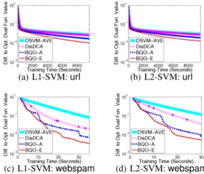
We compare different dual algorithms in terms of the rela-tive dual objecrela-tive function value.
|(f(αt)−f(α∗))/f(α∗)|, (28)
α∗is obtained approximately by running our method with a strict stopping condition. To have a fair comparison with
TRON which solves the primal problem, we also report the relative primal objective function values and the accu-racies relative to the accuracy at the optimum. The pocket approach discussed in Section2.3is adopted in all dual al-gorithms.
We use16nodes in a cluster. Each node has two Intel HP X5650 2.66GHZ 6C Processors, and one core per node is used. The MPI environment is MPICH2 (Gropp,2002).
2
Downloaded from http://www.csie.ntu.edu.tw/ ˜cjlin/libsvmtools/distributed-liblinear/.
(a) L1-SVM:url (b) L2-SVM:url
(c) L1-SVM:webspam (d) L2-SVM:webspam
Figure 1.Time versus relative dual objective value (28).
The statistics of the data sets in our experiments are shown in Table1. All of them are publicly available.3 Instances
are split across machines in a uniform random fashion. We fixC = 1in all experiments for a fair comparison in opti-mization. Therefore, some algorithms may have accuracies exceeding that of the optimal solution because the bestCis not chosen. We note, though, that once parameter selection is conducted, the method that decreases the function value faster should also achieve the best accuracy faster.
Since this work aims at a framework that can accommo-date any local solvers, we use the same local solver set-ting forDisDCA,DSVM-AVEand our algorithm. In par-ticular, at each time of solving (5), we randomly shuffle the instance order, and then let each machine pass through all local instances once. The training time could be im-proved for high-dimensional data if we use more inner iter-ations, but our setting provides a fair comparison by having computation-communication ratios similar toTRON.
3
http://www.csie.ntu.edu.tw/˜cjlin/ libsvmtools/datasets.
(a) L1-SVM:url (b) L2-SVM:url
(c) L1-SVM:webspam (d) L2-SVM:webspam
Figure 2.Time versus relative accuracy. Training Time
(a)epsilon (b)webspam
Training Time + IO Time
(c)epsilon (d)webspam
Figure 3.Speedup of training L2-SVM. Top: training time. Bot-tom: total running time including training and data loading time.
Tables2-3show the results of the primal and dual objective, respectively. More detailed examination of dual objective and relative accuracies are in Figures1-2. Due to space limit, we only present results on two data sets. More results are discussed in the supplement. In most cases, BQO-E
reduces the primal objective the fastest. Moreover,BQO-E
always reduces the dual objective significantly faster than other solvers and almost always reaches stable accuracies the earliest. BecauseBQO-Ais inferior toBQO-Ein most cases, it is excluded from later comparisons.
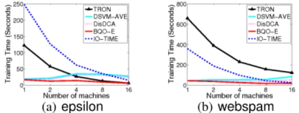
We then examine the speedup of solving L2-SVM using different numbers of machines. In this comparison, we use the two largest data setswebspamandepsilonthat repre-sent the casesl nandn lrespectively. The results are in Figure3. We present both training time speedup and total running time speedup. In both data sets, the training
(a)epsilon (b)webspam
Figure 4.Training time (I/O time excluded) of L2-SVM using dif-ferent numbers of machines.
time speedup of our algorithm is worse than TRON but better than other methods. ButBQO-E has significantly better speedup of overall running time when the I/O time is included. A further investigation of the training time and data loading time in Figure4shows that this running time speedup ofBQO-Eresults from the fact thatBQO-Ehas shorter training time in all cases. Thus, the data loading time is the bottleneck of the running time inBQO-E, and decreasing the data loading time can significantly improve the running time, even if its training time does not improve much with more machines.
From the results above, our method is significantly faster than the state-of-the-art primal solverTRONand all exist-ing distributed dual linear SVM algorithms.
Note that the comparison between DSVM-AVE and
DisDCA accords the results in the results in Ma et al. (2015) that when smallerλ(equivalent to larger weight on the loss term) is used, the difference between the two algo-rithms is less significant. This can also be verified by the re-sult on theurldata set that has largerland thus a larger loss term with a fixedC, which is also equivalent to aλsmaller than that being considered inMa et al.(2015). Additional experiments in the supplement show that for smallerC, the differences are significant andDisDCAis superior. But in these cases, most algorithms finish training in a very short time and thus the setting of smaller C does not provide meaningful comparisons.
5. Conclusions
In this paper, we present an efficient method for distribut-edly solving linear SVM dual problems. Our algorithm is shown to have better theoretical convergence rate and faster empirical training time than state-of-the-art algorithms. We plan to extend this work to problems like structured SVM (Tsochantaridis et al.,2005) where optimizing the primal problem is difficult. Based on this work, we have ex-tended the packageMPI-LIBLINEAR(after version 1.96) at http://www.csie.ntu.edu.tw/˜cjlin/ libsvmtools/distributed-liblinear/ to include the proposed implementation.
Acknowledgment
This material is based on research sponsored by DARPA under agreement number FA8750-13-2-0008. The U.S. Government is authorized to reproduce and distribute reprints for Governmental purposes notwithstanding any copyright notation thereon. The views and conclusions contained herein are those of the authors and should not be interpreted as necessarily representing the official policies or endorsements, either expressed or implied, of DARPA or the U.S. Government.
The authors thank the Illinois Campus Cluster Program for providing computing resources required to conduct experi-ments in this work. We also thank the anonymous review-ers for their comments, and thank Eric Horn for proof-reading the paper. Ching-Pei Lee thanks Po-Wei Wang for fruitful discussion and great help, thanks Chih-Jen Lin, Hsiang-Fu Yu, and Hsuan-Tien Lin for their valuable sug-gestions, thanks Martin Jaggi for the pointer to the conver-gence proof of the practical variant ofDisDCA, and thanks Tianbao Yang for discussion onDisDCA.
References
Agarwal, Alekh, Chapelle, Olivier, Dudik, Miroslav, and Langford, John. A reliable effective terascale linear learning system.Journal of Machine Learning Research, 15:1111–1133, 2014.
Bian, Yatao, Li, Xiong, and Liu, Yuncai. Parallel coordi-nate descent Newton for large-scale L1-regularized min-imization. Technical report, 2014. arXiv:1306.4080v3. Boser, Bernhard E., Guyon, Isabelle, and Vapnik, Vladimir.
A training algorithm for optimal margin classifiers. In
Proceedings of the Fifth Annual Workshop on Computa-tional Learning Theory, pp. 144–152. ACM Press, 1992. Boyd, Stephen, Parikh, Neal, Chu, Eric, Peleato, Borja, and Eckstein, Jonathan. Distributed optimization and statisti-cal learning via the alternating direction method of mul-tipliers. Foundations and Trends in Machine Learning, 3(1):1–122, 2011.
Chang, Kai-Wei and Roth, Dan. Selective block minimiza-tion for faster convergence of limited memory large-scale linear models. InProceedings of the Seventeenth ACM SIGKDD International Conference on Knowledge Discovery and Data Mining, 2011.
Gallant, Stephen I. Perceptron-based learning algorithms.
Neural Networks, IEEE Transactions on, 1(2):179–191, 1990.
Gropp, William. MPICH2: A new start for MPI implemen-tations. InRecent Advances in Parallel Virtual Machine and Message Passing Interface, pp. 7–7. Springer, 2002.
Hazan, Tamir, Man, Amit, and Shashua, Amnon. A paral-lel decomposition solver for SVM: Distributed dual as-cend using Fenchel duality. InProceedings of the IEEE Conference on Computer Vision and Pattern Recognition (CVPR), pp. 1–8. IEEE, 2008.
Hsieh, Cho-Jui, Chang, Kai-Wei, Lin, Chih-Jen, Keerthi, S. Sathiya, and Sundararajan, Sellamanickam. A dual coordinate descent method for large-scale linear SVM. InProceedings of the Twenty Fifth International Confer-ence on Machine Learning (ICML), 2008.
Lin, Chieh-Yen, Tsai, Cheng-Hao, pei Lee, Ching, and Lin, Chih-Jen. Large-scale logistic regression and linear sup-port vector machines using Spark. InProceedings of the IEEE International Conference on Big Data, pp. 519– 528, 2014.
Ma, Chenxin, Smith, Virginia, Jaggi, Martin, Jordan, Michael I, Richt´arik, Peter, and Tak´aˇc, Martin. Adding vs. averaging in distributed primal-dual optimization. In
Proceedings of the 32nd International Conference on Machine Learning (ICML), 2015.
Pang, Jong-Shi. A posteriori error bounds for the linearly-constrained variational inequality problem.Mathematics of Operations Research, 12(3):474–484, 1987.
Pechyony, Dmitry, Shen, Libin, and Jones, Rosie. Solving large scale linear SVM with distributed block minimiza-tion. InNeural Information Processing Systems Work-shop on Big Learning: Algorithms, Systems, and Tools for Learning at Scale, 2011.
Shalev-Shwartz, Shai and Zhang, Tong. Stochastic dual co-ordinate ascent methods for regularized loss minimiza-tion. Journal of Machine Learning Research, 14:567– 599, 2013.
Tseng, Paul and Yun, Sangwoon. A coordinate gradient descent method for nonsmooth separable minimization.
Mathematical Programming, 117:387–423, 2009. Tsochantaridis, Ioannis, Joachims, Thorsten, Hofmann,
Thomas, and Altun, Yasemin. Large margin methods for structured and interdependent output variables. Journal of Machine Learning Research, 6:1453–1484, 2005. Vapnik, Vladimir. The Nature of Statistical Learning
The-ory. Springer-Verlag, New York, NY, 1995.
Wang, Po-Wei and Lin, Chih-Jen. Iteration complexity of feasible descent methods for convex optimization.
Journal of Machine Learning Research, 15:1523–1548, 2014.
Yang, Tianbao. Trading computation for communication: Distributed stochastic dual coordinate ascent. In Ad-vances in Neural Information Processing Systems 26, pp. 629–637, 2013.
Yang, Tianbao, Zhu, Shenghuo, Jin, Rong, and Lin, Yuan-qing. On theoretical analysis of distributed stochastic dual coordinate ascent. Technical report, 2014. arXiv preprint arXiv:1312.1031.
Yu, Hsiang-Fu, Hsieh, Cho-Jui, Chang, Kai-Wei, and Lin, Chih-Jen. Large linear classification when data cannot fit in memory.ACM Transactions on Knowledge Discovery from Data, 5(4):23:1–23:23, February 2012.
Yuan, Guo-Xun, Ho, Chia-Hua, and Lin, Chih-Jen. Recent advances of large-scale linear classification.Proceedings of the IEEE, 100(9):2584–2603, 2012.
Yun, Sangwoon. On the iteration complexity of cyclic coor-dinate gradient descent methods. SIAM Journal on Op-timization, 24(3):1567–1580, 2014.
Zhang, Caoxie, Lee, Honglak, and Shin, Kang G. Efficient distributed linear classification algorithms via the alter-nating direction method of multipliers. InProceedings of the 15th International Conference on Artificial Intel-ligence and Statistics, 2012.
Zhuang, Yong, Chin, Wei-Sheng, Juan, Yu-Chin, and Lin, Chih-Jen. Distributed Newton method for regularized logistic regression. InProceedings of The Pacific-Asia Conference on Knowledge Discovery and Data Mining (PAKDD), 2015.