Differential Evolution-based 3D Directional Wireless Sensor Network Deployment Optimization

(1)

Differential Evolution-based 3D Directional

Wireless Sensor Network Deployment

Optimization

Bin Cao,

Member, IEEE,

Xinyuan Kang, Jianwei Zhao, Po Yang,

Member, IEEE,

Zhihan Lv,

Member, IEEE,

and Xin Liu

Abstract—Wireless sensor networks (WSNs) are applied more and more widely in real life. In actual scenarios, 3D directional wireless sensors (DWSs) are constantly employed, thus, research on the real-time deployment optimization problem of 3D directional wireless sensor networks (DWSNs) based on terrain big data has more practical significance. Based on this, we study the deployment optimization problem of DWSNs in the 3D terrain through comprehensive consideration of coverage, lifetime, connectivity of sensor nodes, connectivity of cluster headers and reliability of DWSNs. We propose a modified differential evolution (DE) algorithm by adopting CR-sort and polynomial-based mutation on the basis of the cooperative coevolutionary (CC) framework, and apply it to address deployment problem of 3D DWSNs. In addition, to reduce computation time, we realize implementation of message passing interface (MPI) parallelism. As is revealed by the experimentation results, the modified algorithm proposed in this paper achieves satisfying performance with respect to either optimization results or operation time.

Index Terms—cooperative coevolution (CC), linear crossover, polynomial-based mutation, differential evolution (DE), 3D directional wireless sensor networks (DWSNs), coverage, lifetime, connectivity, reliability

F

1 I

NTRODUCTION

W

ITH the continuous development of communication technologies and smart sensing devices, the Internet of Things(IoT) provides more and more convenience and efficiency to human living [1]. Wireless sensor networks (WSNs), which are the basic technology of IoT, composed of a certain number of lightweight, low-cost wireless sensor nodes [2], have also experienced great progress. Utilizing the vibration sensors for identification and narrow-band internet of things for communication, Jia et al. [3] proposed an edge computing-based intelligent manhole cover man-agement system. Aguirre et al. [4] applied WSNs to the real-time monitoring of urban traffic environments. Fosalau et al. [5] monitored catastrophic natural phenomena (e.g., landslides) by deploying highly sensitive sensor nodes to perceive the moving direction and displacement of soil.

With the increasingly widespread application of IoT and WSNs, many scholars have studied related issues. Santigo This work was supported in part by the National Natural Science Foundation of China (NSFC) under Grant No. 61303001, in part by the Opening Project of Guangdong High Performance Computing Society under Grant No. 2017060101, in part by the Foundation of Key Laboratory of Machine Intelligence and Advanced Computing of the Ministry of Education under Grant No. MSC-201602A, and in part by the Special Program for Applied Research on Super Computation of the NSFC-Guangdong Joint Fund (the second phase) under Grant No. U1501501. (Corresponding authors: Po Yang, Bin Cao )

Bin Cao, Xinyuan Kang, Jianwei Zhao and Xin Liu are in the Hebei University of Technology, Tianjin, 300401, China; Key Laboratory of Machine Intelligence and Advanced Computing (Sun Yat-sen University), Ministry of Education; Hebei Provincial Key Laboratory of Big Data Calculation, China. (email: [email protected]; [email protected]; [email protected]; [email protected])

Po Yang is in the Department of Computer Science, Liverpool John Moores University, Liverpool, UK. (email: [email protected])

Zhihan Lv is in the School of Data Science and Software Engineering, Qingdao University, Qingdao 266071, China. (email: [email protected])

et al. [6] proposed a modified feature selection algorithm which can separate and prioritize the sensor data and ap-plied to industrial IoT. The deployment problem of WSNs can be well resolved by biological heuristic algorithms. How to improve the coverage and prolong the lifetime of the WSNs are two main research directions. By combining adaptive length coding, Alia et al. [7] presented a novel algorithm that could automatically modify and determine the optimum quantity and positions of sensor nodes to achieve coverage maximization with the cost minimization. Manju et al. [8] proposed a method of setting nodes work alternately and giving coverage priority of crucial moni-toring areas to prolong the network lifetime. Tuba et al. [9] employed the fireworks algorithm [10] to optimize the coverage rate of WSNs, which realized coverage rate maxi-mization via finding “optimum” sensor positions. However, they only researched the deployment problem on 2D plane, while sensor nodes in the real world exist in 3D space, the sensing range of sensors is 3D and has sensing angles limited. Accordingly, directional sensor nodes with limited sensing angles are more accordant with the actual situation. The concept of directional sensors was proposed by Ma et al. [11]. Based on which, Teng et al. [12] proposed a fuzzy ring based fan-shaped sensing model, and this study was more practical. Therefore, research on the deployment problem of directional wireless sensor networks (DWSNs) on 3D terrain has more realistic significance and practical value.

Sung et al. [13] proposed a distributed greedy algorith-m to ialgorith-mprove the coverage of directional sensor nodes. Considering the directionality and sensing angle and com-bining Voronoi diagrams. Nevertheless, only one objective, coverage, was considered. Cao et al. [14] considered the coverage and lifetime of directional sensor nodes in 3D

(2)

industrial space with obstacles, and distributed parallelism was conducted to reduce the computation time.

Node clustering and routing are two well-known meth-ods to prolong lifetime of WSNs [15]. Usually, these two methods are simultaneously employed to improve the en-ergy utilization rate. Halder et al. [16] discovered that the energy imbalance across the network is mainly owes to the data transmission to relay nodes from different sections, and they put forward a heterogeneous node deployment strategy to extend network lifetime. Chu et al. [17] pro-posed a distributed cooperative topology control and adap-tation algorithm to achieve the extend of network lifetime. Hacioglu et al. [18] presented a clustering-based routing methodology, which minimized the communication costs among clusters and maximized the node quantity in each cluster, and NSGA-II [19] was combined to select excellent solutions. However, all these studies only explored the case of 2D plane.

To achieve the data transmission stability in IoT, a stable and reliable network is essential [20]. Connectivity is basic for the reliable data transmission, and it’s basic of the topol-ogy control and routing protocol. Besides the basic coverage and lifetime, connection and reliability [21] also should be concerned to ensure the wireless networks performance. Li et al. [22] proposed a deployment strategy for simultane-ously considering coverage and connectivity based on the elitist non-dominated sorting genetic algorithm (NSGA-II) [19]. Zakia et al. [23] considered the Quality of Monitoring (QoM) and wireless network connectivity and proposed a 3D underwater deployment scheme. [24] considered cover-age, connectivity uniformity and deployment cost, and [24] proposed a distributed parallel cooperative coevolutionary multi-objective large-scale immune algorithm to solve it, while [25] just utilized the existing algorithm, however reliability was both not into consideration. Li et al. [26] im-proved a three-factor user authentication protocol for WSN to satisfy the security requirement in IoT application. Deif et al. [27] proposed a modified Ant Colony Optimization (ACO) to improve the reliability of WSNs at a minimum deployment cost. Machado et al. [28] presented a diffusion-based approach to satisfy the coverage, connectivity and reliability of WSNs, however it is deployed on the 2D plane. Above all, there are few studies simultaneously considered the coverage, lifetime, connectivity and reliability of DWSNs on 3D terrain.

This paper comprehensively considers the coverage, life-time, the connectivity of sensor nodes, the connectivity of cluster headers, and the reliability of fuzzy ring-based DWSNs on 3D terrain. To address it, we present a modified DE algorithm: cooperative coevolutionary (CC) [29] differ-ential evolution (DE) algorithm [30] with CR-sort [31] and polynomial-based mutation (CCDEXSPM). In this paper, our main contributions are as follows:

A. In the process of mutation in DE, we simply select par-ents from the whole population with uniform probabili-ty, ensuring a greater search direction of the population and avoiding premature convergence for falling into local optima. For the crossover factor, we adopt a novel dynamic updating scheme of CR-sort [31].

B. To avoid premature convergence of the population, after the mutation and crossover, we append a

polynomial-based mutation operator to perform a second-time mu-tation to each newly generated individual.

C. We combine the above evolutionary strategy with the novel CC strategy proposed in [32] by adopting fixed grouping [29] and allocating variables of the same prop-erty to the same group to improve optimization efficien-cy.

D. To improve the operation speed, message passing inter-face (MPI) parallelism is adopted.

The rest of the article is arranged as follows: Section 2 presents related concepts. Our work is detailed in Section 3. The experiments and analysis are provided in Section 4. Finally, we conclude this paper in Section 5.

2 R

ELATED

C

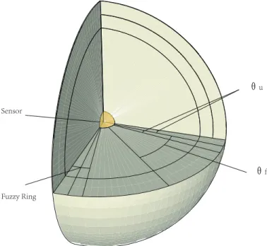
ONCEPTS 2.1 WSN Sensing Model

According to the shape of the coverage region, the sensing model can be classified as: omni-directional sensing model and directional sensing model. Traditional sensor nodes are generally omni-directional sensor nodes, the sens-ing range of which is a spherical region.For directional sensor nodes, the sensing range is limited with respect to the horizontal sensing angle,as illustrated in Fig. 1, the deterministic sensing angle is(θf−θu)and the angle range of the fuzzy ring is2θu.

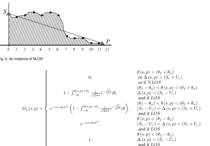
If a pointpcan be detected by a sensor nodes, the Line-of-Sight (LOS) is satisfied with respect tosandp, and Fig. 2 is an instance of non-LOS (NLOS). Considering of LOS, the sensing range [12] of directional sensor nodes can be represented as Eq. 1.

2.2 Coverage Degree

The sensing probability of a certain point is influenced by its distance from the sensor node. This paper adopts multi-point coverage strategy and the Sugeno measure [33],

Sensor

θf

θu

Fuzzy Ring

(3)

Fig. 2. An instance of NLOS. Oq(s, p) =                                                    0, θ(s, p)>(θf+θu) or∆ (s, p)>(Sr+Ur) or ifN LOS 1−Rθ(s,p)−θf −∞ 1 √ 2πσe −t2 2σ2_dt, (θf−θu)< θ(s, p)<(θf+θu) ∆ (s, p)<(Sr−Ur) and ifLOS e−α×distβ 1−Rθ(s,p)−θf −∞ 1 √ 2πσe −t2 2σ2_dt , (θf−θu)< θ(s, p)<(θf+θu) (Sr−Ur)<∆ (s, p)<(Sr+Ur) and ifLOS e−α×distβ_, θ(s, p)<(θf−θu) (Sr−Ur)<∆ (s, p)<(Sr+Ur) and ifLOS 1, θ(s, p)<(θf−θu) ∆ (s, p)<(Sr−Ur) and ifLOS (1)

whereθ(s, p)is the angle between the main sensing direction of sensor nodesand the line connecting sensor nodesand pointp.

[34] to describe the uncertain coverage of WSNs, which can be detailed as follows: Oq(p) = min 1, 1 λ ( _n Y k=1 [1 +λ×Oq(sk, p)]−1 )! (2) where n denotes the number of sensor nodes and λ (−1≤λ <0)is the fusion operator [35]. LetOthdenote the coverage degree threshold. To evaluate the coverage degree, define [35]: Os(p) = 1, Oq(p)≥Oth 0, otherwise (3) QoC= 1 P P X j=1 Os(pj) (4)

where QoC denotes the quality of coverage of the target region after each deployment andPis the number of points.

2.3 Lifetime Model

2.3.1 Energy Consumption Model

The radio energy consumption model we adopt is the same as in [15]. By setting the distance threshold dth and adopting different energy consumption patterns, the specific equation for transmission is in the following:

ET(l, d) =

lEelec+lεf sd2, d < dth

lEelec+lεmpd4, d≥dth (5) wherelis the message quantity with the unit ofbit,Eelec de-notes the energy consumption parameter, andεf sandεmp are parameters in the free-space and multi-path channels, respectively. The energy consumption for receiving l bit messages, can be calculated as follows:

ER(l) =lEelec (6) 2.3.2 Lifetime Model of CHs

The energy consumption model of sensor nodesEsensor is composed of two parts: sensing energy consumption Esense, and communication energy consumptionEcom for transmitting data to CHs, which can be formulated as:

Esensor=Esense+Ecom (7) The energy consumption Eclu(gi)within the cluster of CHgi contains three majors consumptions: the Erec,Eagg and Esend represent the energy consumption of receiving, aggregating and sending one bit data, respectively :

1) The energy consumption of receivingl0-bit data from

(4)

2) The energy consumption of aggregating thel0-bit data

of allrisensor nodes in the cluster reachesril0Eagg.

3) The energy consumption of transmitting l0-bit data

with the distancediwill be:

l0Esend=

l0Esend+l0εf sd2i, di < dth

l0Esend+l0εmpd4i, di ≥dth (8) A compression ratiorcmpis set to represent the degree of data aggregation. The energy consumed for transmit-ting data received fromrisensor nodes to the next hop will berircmpl0Esend.

Therefore, the energy consumptionEclu(gi)of CHgi in its own cluster can be represented as:

Eclu(gi) =ril0(Erec+Eagg+rcmpEsend) (9) For a relay node gi, the energy consumption Egateway(gi)for relaying data of other CHs mainly includes two aspects:

1) Energy consumption for receiving data of si sensor nodes from the previous hop will besircmpl0Erec.

2) Energy consumption for relaying data of si sensor nodes will besircmpl0Esend.

Therefore, the energy consumption Egateway of relay nodegi for relaying data for other CHs can be represented as:

Egateway(gi) =sircmpl0(Erec+Esend) (10) Finally, the energy consumption E(gi)of relay nodegi can be denoted as:

E(gi) = Eclu(gi) +Egateway(gi)

= ril0(Erec+Eagg+rcmpEsend) + sircmpl0(Erec+Esend)

= (ri+sircmp)l0Erec+ ril0Eagg+

(ri+si)rcmpl0Esend

(11)

The WSN lifetime adopts the pattern ofN-of-N, that is, the lifetime of the whole WSN vanishes when the first CH exhausts its energy.

Assuming that residual energy of CHgiisEresidual(gi), its lifetimeL(i)can be represented as:

L(i) =Eresidual(gi)

E(gi)

(12)

2.4 Network Connectivity

WSNs accomplish the monitoring task mainly through gathering and transferring information and data. All nodes cooperate with each other to guarantee the normal oper-ation of the WSNs. Therefore, the network connectivity is an important guarantee of the network functionality. Each sensor node selects one CH to join its cluster and transmits the gathered information to its CH. Then, the CHs aggregate the data transferred from sensor nodes in the clusters and relay them to the next hops. We considered the connectivity of CHs and sensor nodes, respectively.

For the CHs, we can guarantee each two CHs perform communication directly or indirectly via other CHs, that is, the number of CHs in the maximal connected set of the whole network is supposed to be the CH number in the network. The uniformity of the numbers of CHs that all CHs can communicate with should be optimized. The standard deviation can be utilized to measure the uniformity [36]:

fU niOf CH = 1 1 +fstd CH (13) fCHstd = s PMCH i=1 (ci−ACH) 2 MCH (14) ACH = PMCH i=1 ci MCH (15) where fU niOf CH is the measure ofConnectivity Uniformity of CH; f_CHstd denotes the standard deviation; MCH is the number of CHs in the largest connected subcomponent,ciis the number of CHs for the CHican communicate with, and ACH is the average value of the number of CHs that each CH can communicate with in the set. If the size of the largest connected set is less than the total number of CHsNCH, a penalty will be assigned which is expressed as follows:

penalty(NCH, MCH) (16) wherepdenotes the penalty factor, which is assigned a great value (e.g.1e6).

For the sensor nodes, to measure the connectivity uni-formity of sensor nodes, we can guarantee the uniuni-formity of the distances of all sensor nodes to their corresponding CHs as far as possible, which can be achieved through utilizing the standard deviation. The specific formula of is as follows:

fU niOf DS= 1 1 +fstd DS (17) fDSstd = s PNDS i=1 (di−ADS) 2 NDS (18) ADS = PNDS i=1 di NDS (19) wherefU niOf DSis the measure ofConnectivity Uniformity of sensor nodes;NDS is the number of sensor nodes, di is the distance of sensor nodei to its corresponding CH,ADS is the average distance of sensor nodes to the CHs.

2.5 Network Reliability

The number of nodes is limited and WSNs are usually applied in sever and complicated environments. When one sensor node corrupts or depletes its energy, coverage holes may occur and a part of the area cannot be sensed; when this happens to a CH, the information gathered by sensor nodes in this cluster and the data transferred from the previous hop would be unsuccessful. More seriously, when this CH is located in the crucial position, the normal operation of the whole network will be influenced. Therefore, the net-work reliability is an important guarantee of the netnet-work functionality. The reliability issue has become a research hot spot of WSNs.

(5)

To alleviate this situation, through employing the method of multi-hop communication, each CH and each sensor node are associated to several CHs. So if the selected CH of the current node corrupts or depletes the energy, another CH can be chosen for information forwarding, thus the whole network can still work normally.

To guarantee the network reliability, we prescribe an average number of CHs that all sensor nodes and CHs can communicate with, shown as follows:

fRel= PNDS i=1 ci+ PNCH j=1 cj (NDS+NCH) 2 (20)

whereciandcj is the number of CHs of sensor nodeiand CHjcan communicate with, respectively.

Moreover, we set a limit of the minimum number of CHs each node should communicate with, as is shown in Eq. 21:

NCH DS ≥2 NCH CH ≥2 (21) whereNCH DS andN CH

CH denote the number of associated CHs of each sensor node and each CH, respectively.

2.6 Objective Function

We have considered the quality of coverage, lifetime, the connectivity uniformity of sensor nodes, the connectivity uniformity of CHs, and the reliability of the WSN, and these five aspects have different importance degrees, we fuse these five aspects by setting different weight value and obtain the final objective function, as follows:

cost= st1×QoC+ st2×Lmin+ st3×fU niOf CH+ st4×fU niOf DS+ st5×fRel (22) s.t.    penalty(NCH, MCH) NCH S ≥2 NCH CH ≥2

wherest1,st2,st3,st4 andst5 are the weight factors, and

Lmin denotes the lifetime of the first CH that exhausts its energy.

3 O

UR

W

ORKS

3.1 Directional Sensing Model

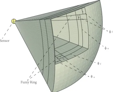
In the 3D directional sensing model [12] mentioned in subsection 2.1, although the horizontal angle constraint is considered, the vertical one should also be taken into account. On the basis of the sensing model presented in [12], we add a vertical angle constraint and put forward a modified 3D directional sensing model.

As to the sensing probability with respect to the distance constraint, we use the same calculation method as in [37], which is detailed in Eq. 23. For the horizontal and vertical angle constraints, we adopt the same probability computa-tion method, as shown in Eq. 25:

Sensor Fuzzy Ring θu θf φf φu

Fig. 3. Modified directional sensing model.

Oq(s, p) =              1, ∆ (s, p)<(Sr−Ur) and ifLOS e−α×distβ, (Sr−Ur)≤∆ (s, p)<(Sr+Ur) and ifLOS 0, ∆ (s, p)>(Sr+Ur) or ifN LOS (23) dist= ∆ (s, p)−(Sr−Ur) (24) Oq(s, p) =              0, γ > γf+γu or NLOS 1−Rγ−γf −∞ √₂1_πσe −t2 2σ2dt, γf−γu < γ < γf+γu and LOS 1, γ < γf−γu and LOS (25) where γ can be the horizontal angle θ or the vertical angle φ, γf and γu are the sensing angles, the radius of the deterministic sensing angle range is(γf−γu), and the radius of the fuzzy ring is2γu, that is to say, the fuzzy ring region is within the angle range of(γf −γu)and(γf+γu). By comprehensively considering the horizontal and vertical angle constraints, we can obtain the modified directional sensing model, as illustrated in Fig. 3.

The specific sensing probability formula is in Eq. 26.

3.2 Routing Algorithm

In the considered WSN, we deploy sensor nodes and relay nodes simultaneously. Each time their positions are determined, we apply the routing algorithm to identify the CH each sensor node belongs to and the routing informa-tion of CHs to the BS. After the informainforma-tion collecinforma-tion of all sensor nodes, the data are transmitted to their CHs. After the CHs receive the data, the residual information is discarded through compression, and the aggregated data will be transmitted to the next hop or BS according to the

(6)

Oq(s, p) =                                                                                                                  1, ∆ (s, p)<(Sr−Ur) θ(s, p)<(θf−θu) φ(s, p)<(φf−φu) and LOS e−α×distβ, (Sr−Ur)<∆ (s, p)<(Sr+Ur) θ(s, p)<(θf−θu) φ(s, p)<(φf−φu) and LOS 1−Rθ(s,p)−θf −∞ 1 √ 2πσe −t2 2σ2_dt, ∆ (s, p)<(Sr−Ur) (θf−θu)< θ(s, p)<(θf+θu) φ(s, p)<(φf−φu) and LOS 1−Rφ(s,p)−φf −∞ 1 √ 2πσe −t2 2σ2_dt, ∆ (s, p)<(Sr−Ur) θ(s, p)<(θf−θu) (φf−φu)< φ(s, p)<(φf+φu) and LOS e−α×distβ 1−Rθ(s,p)−θf −∞ 1 √ 2πσe −t2 2σ2_dt , (Sr−Ur)<∆ (s, p)<(Sr+Ur) (θf−θu)< θ(s, p)<(θf+θu) φ(s, p)<(φf−φu) and LOS e−α×distβ 1−Rφ(s,p)−φf −∞ 1 √ 2πσe −t2 2σ2_dt , (Sr−Ur)<∆ (s, p)<(Sr+Ur) θ(s, p)<(θf−θu) (φf−φu)< φ(s, p)<(φf+φu) and LOS 1−Rθ(s,p)−θf −∞ 1 √ 2πσe −t2 2σ2_dt ₁₋Rφ(s,p)−φf −∞ 1 √ 2πσe −t2 2σ2_dt , ∆ (s, p)<(Sr−Ur) (θf−θu)< θ(s, p)<(θf+θu) (φf−φu)< φ(s, p)<(φf+φu) and LOS e−α×distβ 1−Rθ(s,p)−θf −∞ 1 √ 2πσe −t2 2σ2_dt ₁₋Rφ(s,p)−φf −∞ 1 √ 2πσe −t2 2σ2_dt , (Sr−Ur)<∆ (s, p)<(Sr+Ur) (θf−θu)< θ(s, p)<(θf+θu) (φf−φu)< φ(s, p)<(φf+φu) and LOS 0, otherwise (26) whereSrandUr denote two distance ranges of sensor nodes, respectively, here, the radius of the deterministic sensing distance is(Sr−Ur), and the radius of the fuzzy ring is2Ur, that is, it locates in the ring between(Sr−Ur)and(Sr+Ur); θf andθu are two horizontal angle ranges, here, the radius of the horizontal deterministic sensing angle is(θf−θu), and the radius of the fuzzy ring is2θu, that is, the horizontal fuzzy ring region is between the angle ranges of(θf−θu)and

(θf+θu);φfandφuare two vertical angle ranges, here, the radius of the deterministic sensing angle is(φf−φu), and the radius of the fuzzy ring is2φu, that is, the angle range between(φf−φu)and(φf +φu)is the vertical fuzzy ring region.

routing algorithm. The specific routing algorithm is detailed in Algorithm 1.

First, we cluster all sensor nodes by allocating each sensor node to its nearest CH, which can reduce the energy consumption of data transmission. Then the routing path will be determined. Specifically, for each CH, its distances to the BS and other CHs are calculated, and the CHs are sorted in descending order according to their distances to the BS. This sorting is important, because we check each CH from far to near, which is convenient for calculating the relayed data for each relay node. Each CH chooses the closest CH as its next hop from those that are nearer to the BS, thus preventing choosing the nearest one which is located farther from the BS and increasing the length of the relaying path.

3.3 Modified Differential Evolution Algorithm

We propose a modified DE algorithm [30] with CR-sort [31] and polynomial-based mutation by combining a novel CC strategy, denoted as CCDEXSPM. The work of [32] utilized the dynamic grouping method [38] into separate variables to several groups constantly and randomly. They

used the optimizer of particle swarm optimization (PSO) [39], and a context vector (i.e., the global best solution) was maintained. Variables in the allocated group updated their values according to the velocity updating formula of PSO; while the remaining variables came from the personal bests or the global best according to several predefined thresholds, but the velocity updating formula was not used. Meanwhile, they utilized another PSO operator to update the context vector.

We combine this CC scheme with our DE strategy. Ac-cording to the characteristics of the deployment problem, we adopt fixed grouping [29] to divide variables into several groups of unequal dimensions by separating variables of the same property into the same group, and each group is optimized in turn. Variables in the current optimization group are mutated, while other variables are the crossover result of the personal best and the global best.

The selection mechanism we utilized is to uniformly choose individuals from the current population for par-ents, ensuring a wider search direction, and avoiding being trapped into local optima and resulting in premature

(7)

con-Algorithm 1:Routing

Input: Coordinates of all sensor nodes and CHs; number of sensor nodesNDS, number of CHs NCH.

Output: Routing scheme. Initialization;

fori= 0toNDS−1do

forj = 0toNCH−1do

Calculate the distance ofi-th sensor node and j-th CH;

end

Choose the closest CH as its own CH;

end

Calculate the distance ofj-th CH and BS;

Calculate the distances ofj-th CH and other CHs;

end

Sort the distances of all CHs with BS in descending order;

For each CH, from those CHs that are closer to the BS, choose the closest CH as its next hop, while for the CH closest to the BS, choose the BS;

end

vergence. This mutation is detailed in Eq. 27: v_i,jg =xg_r₁_,j +Fi×

xg_r₂_,j−xg_r₃_,j s.t. j∈Svarm

(27) wherexg_r₁,xg_r₂andxg_r₃are randomly and uniformly selected from theg-th generation of population, here1≤g ≤gmax and gmax is the maximum generation quantity, j is the variable. Sm

var is the set of variables to be optimized in subpopulationm, here1 ≤m ≤M andM is the number of subpopulations. The scale factor Fi of each individual follows the updating scheme in JADE [40], which satisfies Cauchy distribution within the range of [0,1] with the position value of µF and the scale parameter of 0.1, as follows in Eq. 28.

Fi=CauchyRandom(µF,0.1) (28) whereµF has an initial value of0.5. LetSF denote the set of allF values of individuals that are successfully mutated, then we can updateµF as in Eq. 29:

µF = (1−c)×µF+c×meanL(SF) (29) wheremeanL(•)represents the Lehmer mean, as in Eq. 30:

meanL(SF) = P F∈SF F 2 P F∈SFF (30) After the mutation of variables in the current group, we integrate the remaining variables. The remaining variables do not come directly from the global best, instead, each individual stores its personal best. Therefore, we randomly select variables from the global best and the personal best,

that is, we conduct crossover between the global best and the personal best, as in Eq. 31:

vg_i,j= xg_i,j, r > CRi Bestj, r≤CRi s.t. j /∈Sm var (31) r=rand() (32)

The crossover rate is determined by CR. For the crossover factor CR, we adopt the updating strategy of CR-sort in [31]. The generation of CR satisfies Gaussian distribution, and after the initial population randomly gen-erated, the fitness of individuals are calculated and ranked in order of best to worst, and the values of CR are sorted in increasing order. Then the better individual would be assigned the smaller value of CR, which helps maintain the better personal best.

To avoid the population from premature convergence, after one mutation of variables in the current group and the generation of the remaining variables from crossover, we add a polynomial-based mutation operator, executing a second-time mutation to the generated individual to improve the diversity of the population. Henceforth, one individual accomplishes its evolution process. As to the polynomial-based mutation operator, we will make detailed introduction in Subsection 3.4.

When each individual in each subpopulation finishes one evolution process, we consider the whole population completes one evolution. The whole population continuous-ly repeats this evolutionary cycle until the termination con-dition is satisfied. The whole evolution process is detailed in Algorithm 2.

3.4 Polynomial-based Mutation

To increase the diversity of the population, avoid pre-mature convergence and being trapped in local optima, after we have conducted mutation and crossover of each individual, a polynomial-based mutation operator is uti-lized to perturb variables selected by a certain probability to conduct a second-time mutation. The polynomial-based mutation perturbs the original value by exerting a small change, improving the diversity of the population [41]. This change valuevperm_i,j can be represented as:

vperm_i,j =σi,j×Bj (34) where i denotes individual i,j represents variablej, and Bj represents the baseline value, which is generally set as

(ubj, lbj), hereubjandlbj are the upper and lower bound-aries of variablej, respectively, andσi,jis the variation ratio, which can be calculated as follows:

σi,j=      h 2u+ (1−2u)×σ_i,j,n+1₁i 1 n+1 −1, ifu≤0.5 1−h2 (1−u) + (2u−1)×σ_i,j,n+1₂i 1 n+1 , otherwise (35) whereuis a random number obeying uniform distribution, n denotes the mutation distribution index, and σi,j,1 and

(8)

Algorithm 2:CCDEXSPM

Output: The final best vector:Best. Initialize();

do

forall individuals in each subpopulationdo

(1) Variables allocated to current subpopulation — mutation according to Eq. 27; (2) Remaining variables in current subpopulation — crossover according to Eq. 31; (3) Generated individual — polynomial-based mutation;

(4) Selection:

xg_i+1=

vg_i, v_ig.cost > xg_i.cost

xg_i, otherwise (33)

wherexg_i andxg_i+1are the personal bests of theg-th and(g+ 1)-th generations, respectively; (5) UpdateFiandCRi;

(6) Update the vector:Best;

end

whileThe termination condition is not met;

σi,j,1= xi,j−lbj ubj−lbj (36) σi,j,2= ubj−xi,j ubj−lbj (37) wherexi,jis the original value before mutation.

Finally, we can obtain the mutated valuex0_i,j:

x0_i,j =xi,j+v perm

i,j (38)

3.5 Parallelism Implementation

To improve the operation speed of the algorithm , we put forward a MPI-based distributed parallel algorithm. In designing the parallel strategy, we observed that the computation of QoC occupied a large proportion of the overall operation time, which includes multiple loops and the time complexity isO(LEN×W ID×DS), hereLEN andW IDrepresent the length and width of the terrain data, respectively. Thus, compared to the communication cost among processes, the computation cost ofQoC is tremen-dous. Especially, when the terrain area expands and the number of sensor nodes increases (that is, the dimensional-ity of the feasible solution is enlarged), the corresponding time consumption will also increase rapidly. Considering these factors, we chiefly divide the computation process into multiple blocks and address them in parallel; then, the information transmission is completed through communi-cation among processes. Specifically, it is to divide the data for computation according to the number of processes. The more the processes, the less the data to be processed in each block. The specific process is in Algorithm 3.

4 E

XPERIMENTAL

R

ESULTS AND

A

NALYSIS

To assess the performance of the novel algorithm, we import real digital elevation model (DEM) raw data1_{. Then,}

1. Geospatial Data Cloud, Computer Network Information Center, Chinese Academy of Sciences. (http://www.gscloud.cn).

Algorithm 3:Parallelism Implementation MPI Init(&argc, &argv);

MPI Comm rank(MPI COMM WORLD,&rank); MPI Comm size(MPI COMM WORLD,&size); block size=len/size;

begin row=rank×block size; end row= (rank+ 1)×block size; MPI Bcast();

fora:=begin row→end rowdo forb:= 0→widdo

Computelocal qoc;

end end

MPI Gatherlocal qoc; MPI Finalize(); return cover();

we crop the DEM data to obtain three terrain data: moun-tainous, hilly and plain terrain data. Through resampling and pretreatment, we obtain three different type of terrain data with a size of 160m×160m and the resolution of

5m. We will use these three types of 3D terrain data for experimentation. The plain, hilly, and mountainous terrain region that we extracted are illustrated in Fig. 4a, Fig. 4b, and Fig. 4c, respectively.

We implement MPI parallelism on the platform of Tianhe-2 supercomputer and conduct experiments on three terrains: plain, hilly and mountainous terrains. We compare the modified algorithm, CCDEXSPM, with MS-DE [42], jDE [43], GPSO [44], and CLPSO [45]. For the deployment problem, each algorithm repeats the operation 20 times. The parameter settings are listed in Table 1. We conduct experiments on the plain, hilly and mountainous terrains, and the results corresponding to nonparametric tests are shown in the following.

For the test results of the plain terrain, as shown in Table 9, our algorithm CCDEXSPM possesses superiority throughout the entire evolutionary process, and the mean fitness values have remained ahead, which gradually

(9)

reach-(a) Plain Terrain (b) Hilly Terrain (c) Mountainous Terrain

Fig. 4. Three types of extracted terrains. TABLE 1 Parameter Settings

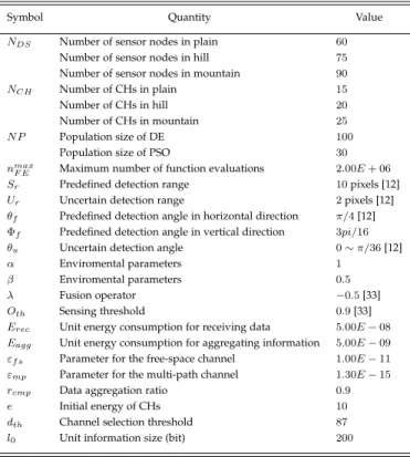
Symbol Quantity Value

NDS Number of sensor nodes in plain 60

Number of sensor nodes in hill 75

Number of sensor nodes in mountain 90

NCH Number of CHs in plain 15

Number of CHs in hill 20

Number of CHs in mountain 25

N P Population size of DE 100

Population size of PSO 30

nmax

F E Maximum number of function evaluations 2.00E+ 06

Sr Predefined detection range 10pixels [12]

Ur Uncertain detection range 2pixels [12]

θf Predefined detection angle in horizontal direction π/4[12] Φf Predefined detection angle in vertical direction 3pi/16

θu Uncertain detection angle 0∼π/36[12]

α Enviromental parameters 1

β Enviromental parameters 0.5

λ Fusion operator −0.5[33]

Oth Sensing threshold 0.9[33]

Erec Unit energy consumption for receiving data 5.00E−08 Eagg Unit energy consumption for aggregating information 5.00E−09 εf s Parameter for the free-space channel 1.00E−11 εmp Parameter for the multi-path channel 1.30E−15

rcmp Data aggregation ratio 0.9

e Initial energy of CHs 10

dth Channel selection threshold 87

l0 Unit information size (bit) 200

es8.57E−01gradually, far higher than the other four algo-rithms,and the maximum fitness value reaches8.79E−01. Similarly, from Fig. 5, we can observe that in the initial stage of evolution, GPSO has encountered premature convergence and is trapped in local optima, while CLPSO, jDE and MS-DE have poor convergence ability, although they have not converged so early, their exploration abilities are inferior to that of our algorithm, as their improvement of the fitness values are slow. In contrast, CCDEXSPM not only has con-verged early in the initial stage of evolution but also has a strong global search capability and updates the fitness value toward the global best solution. In the late stage of evolution, it performs the local search around the global best, and it finally achieves optimization results that are much better than those of the other four algorithms. For the Friedman test in Table 2, the rank of CCDEXSPM is ahead of the other four algorithms. Moreover, from results of the Wilcoxon test in Table 3, we find that all results

achieved by CCDEXSPM are better than those of the other four algorithms (Exact P −valueis equal to 1.91E−06

compares to CLPSO, GPSO, jDE, and2.67E−05to MS-DE). In brief, the optimization performance of our algorithm is significantly better than that of GPSO, CLPSO, jDE and MS-DE.

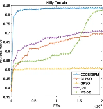
Regarding the test results of the hilly terrain, as shown in Table 10 and Fig. 6, GPSO, CLPSO and jDE have sim-ilar performance compared to plain terrain, while MS-DE exhibits better performance, especially in the late stage of evolution. However, these four algorithms still show weak exploration ability (MS-DE performs better search ability) ; in contrast, our algorithm CCDEXSPM still exhibits strong exploration ability compared to the other four algorithms. For the Friedman test in Table 4, the rank of CCDEXSPM is still ahead of the other four algorithms, and the rank of GPSO is still the last one. From results of the Wilcoxon test in Table 5, we find that all results achieved by CCDEXSPM are

(10)

FEs _×₁₀6 0 0.5 1 1.5 2 Fitness Value 0.35 0.4 0.45 0.5 0.55 0.6 0.65 0.7 0.75 0.8 0.85 0.9 Plain Terrain CCDEXSPM CLPSO GPSO jDE MS-DE

Fig. 5. Test results on plain terrain. TABLE 2

Friedman Test Results (Plain)

Algorithm Ranking CLPSO 3.1 GPSO 5 MS-DE 2.1 jDE 3.7 CCDEXSPM 1.1 TABLE 3

Wilcoxon Test Results (Plain)

VS R+ R- Exact P-value Asymptotic P -value

CLPSO 210 0 1.91E-06 0.000082

GPSO 210 0 1.91E-06 0.000082

MS-DE 204 0 2.67E-05 0.000204

jDE 210 0 1.91E-06 0.000082

still better than those of the other four algorithms (Exact P −value is equal to 1.91E −06). These indicate the effectiveness of CCDEXSPM in hilly terrain.

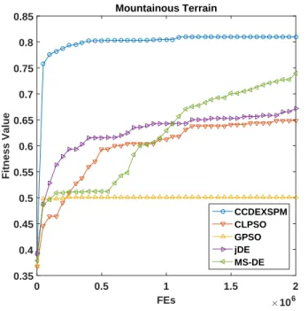
For the mountainous terrain, as shown in Table 11 that these five algorithms show similar performance to that corresponding to plain terrain. The overall fitness values have decreased to some extent (the mean fitness reach-es 8.57E-01 in plain terrain, while it is only 7.86E-01 in mountainous terrain). This result is mainly because that the undulating terrain obstruct the LOS, and the coverage, lifetime, connectivity of nodes will be affected to varying degrees. However, CCDEXSPM has still achieved evident superiority. The Friedman test in Table 6 shows that the rank of CCDEXSPM is still ahead of the other four algorithms,

FEs _×₁₀6 0 0.5 1 1.5 2 Fitness Value 0.35 0.4 0.45 0.5 0.55 0.6 0.65 0.7 0.75 0.8 0.85 Hilly Terrain CCDEXSPM CLPSO GPSO jDE MS-DE

Fig. 6. Test results on hilly terrain. TABLE 4 Friedman Test Results (Hill)

Algorithm Ranking CLPSO 3.85 GPSO 5 MS-DE 2.1 jDE 3.05 CCDEXSPM 1 TABLE 5 Wilcoxon Test Results (Hill)

CLPSO 210 0 1.91E-06 0.000082

GPSO 210 0 1.91E-06 0.000082

MS-DE 210 0 1.91E-06 0.000082

jDE 210 0 1.91E-06 0.000082

and the results of Wilcoxon test in Table 7 also indicate the excellent optimization performance of our algorithm.

The experimental results prove that our algorithm ex-hibits better performance that the other four algorithms in three different terrains. The different terrains would affect the fitness values, and the obtained fitness values on the mountainous terrain are inferior to those on the plain ter-rain. However, our algorithm exhibits stable search ability in different terrain and obtains satisfactory results in fitness. To verify the effect of MPI parallelism on reducing the com-putational time, for the deployment problem on the plain terrain, we conduct experiments by utilizing CCDEXSPM in the cases of 1, 2, 4,8 and 16processes. The experimental results are listed in Table 8 and Fig. 8.

(11)

FEs _×₁₀6 0 0.5 1 1.5 2 Fitness Value 0.35 0.4 0.45 0.5 0.55 0.6 0.65 0.7 0.75 0.8 0.85 Mountainous Terrain CCDEXSPM CLPSO GPSO jDE MS-DE

Fig. 7. Test results on mountainous terrain. TABLE 6

Friedman Test Results (Mountain)

Algorithm Ranking CLPSO 3.7 GPSO 5 MS-DE 2.2 jDE 3.1 CCDEXSPM 1

As shown, as the number of processes increases, the overall operation time significantly decreases. When the number of processes is16, the speedup ratio reaches approx-imately12; however, with a greater number of processes, the use efficiency of each process is lower. When the number of processes is16, the use efficiency of each process is reduced from approximately 0.97 for 2 processes to approximately

0.74. Therefore, if the number of processes further increases, computational resources will not be effectively explored due to the increased communication cost among MPI processes and the low use efficiency of each process. When the number of processes is16, the operation time is effectively reduced, obtaining satisfactory results in operation time.

5 C

ONCLUSION

In this paper, we have primarily studied the deployment problem of DWSNs, we consider the coverage, lifetime, connectivity of sensor nodes, connectivity of CHs, and reliability in the deployment. We propose a modified DE algorithm with CR-sort and polynomial-based mutation by combining the CC framework, namely CCDEXSPM. We ap-ply this algorithm to the deployment optimization problem

TABLE 7

Wilcoxon Test Results (Mountain)

CLPSO 210 0 1.91E-06 0.000082 GPSO 210 0 1.91E-06 0.000082 MS-DE 210 0 1.91E-06 0.000082 jDE 210 0 1.91E-06 0.000082 TABLE 8 Operation Times

Process quantity Average operation time (s) Speedup ratio Efficiency

1 21772.10823 1 1

2 11163.08569 1.950366 0.975183

4 6022.174545 3.615323 0.903831

8 3406.991099 6.390421 0.798803

16 1845.148276 11.799652 0.737478

Number of MPI Processes

1 2 4 8 16

Average Time Consumption (s)

×104 0 0.4 0.8 1.2 1.6 2 2.4 Time Comparison Speedups 0 2 4 6 8 10 12

Average time consumption Actual speedups

Fig. 8. Operation times.

of DWSNs, and compare it with GPSO, CLPSO, jDE and MS-DE. The experimental results show that the the performance of our modified DE algorithm is significantly better than that of these four algorithms. Additionally, we utilize MPI parallelism, effectively reducing the operation time.

For future research, there is still considerable work needs to be performed. We utilize weighted sum to combine the coverage rate, lifetime, connectivity of sensor nodes, connec-tivity of CHs, and reliability to a single objective function, while further research can be conducted by exploring multi-objective optimization.

(12)

TABLE 9

Algorithm Comparison Results (Plain)

FEs CLPSO GPSO jDE MSDE CCDEXSPM 5.00E+05

MEAN 6.34E-01 5.12E-01 6.94E-01 6.10E-01 8.53E-01 MAX 6.52E-01 5.51E-01 7.14E-01 6.91E-01 8.74E-01 MIN 6.18E-01 4.66E-01 6.77E-01 5.80E-01 8.42E-01 MEDIAN 6.35E-01 5.12E-01 6.93E-01 5.94E-01 8.51E-01 STD 8.77E-03 2.22E-02 9.39E-03 3.34E-02 8.25E-03 1.00E+06

MEAN 7.06E-01 5.12E-01 7.27E-01 6.86E-01 8.54E-01 MAX 7.34E-01 5.51E-01 7.41E-01 7.66E-01 8.45E-01 MIN 6.94E-01 4.66E-01 7.16E-01 5.94E-01 8.68E-01 MEDIAN 7.03E-01 5.12E-01 7.26E-01 6.75E-01 8.54E-01 STD 1.06E-02 2.24E-02 7.99E-03 4.57E-02 8.22E-03

1.50E+06

MEAN 7.47E-01 5.12E-01 7.49E-01 7.59E-01 8.56E-01 MAX 7.62E-01 5.51E-01 7.65E-01 8.34E-01 8.78E-01 MIN 7.39E-01 4.66E-01 7.37E-01 6.56E-01 8.45E-01 MEDIAN 7.47E-01 5.12E-01 7.48E-01 7.62E-01 8.55E-01 STD 5.87E-03 2.24E-02 8.94E-03 4.66E-02 8.18E-03

2.00E+06

TABLE 10

Algorithm Comparison Results (Hill)

1.00E+06

1.50E+06

2.00E+06

(13)

TABLE 11

Algorithm Comparison Results (Mountain)

MEAN 5.20E-01 4.29E-01 5.57E-01 4.27E-01 7.79E-01 MAX 5.35E-01 4.85E-01 5.71E-01 4.47E-01 8.18E-01 MIN 5.06E-01 3.85E-01 5.40E-01 4.14E-01 7.59E-01 MEDIAN 5.18E-01 4.28E-01 5.56E-01 4.26E-01 7.76E-01 STD 8.00E-03 2.51E-02 8.45E-03 7.78E-03 1.49E-02

1.00E+06

1.50E+06

2.00E+06

R

EFERENCES

[1] M. Chernyshev, Z. Baig, O. Bello, and S. Zeadally, “Internet of things (iot): Research, simulators, and testbeds,”IEEE Internet of Things Journal, vol. PP, no. 99, pp. 1–1, 2017.

[2] K. Wu, Y. Gao, F. Li, and Y. Xiao, “Lightweight deployment-aware scheduling for wireless sensor networks,” Mobile Networks and Applications, vol. 10, no. 6, pp. 837–852, Dec 2005.

[3] G. Jia, G. Han, H. Rao, and L. Shu, “Edge computing-based intelligent manhole cover management system for smart cities,”

IEEE Internet of Things Journal, vol. PP, no. 99, pp. 1–1, 2017. [4] E. Aguirre, P. Lopez-Iturri, L. Azpilicueta, A. Redondo, J. J.

Astrain, J. Villadangos, A. Bahillo, A. Perallos, and F. Falcone, “Design and implementation of context aware applications with wireless sensor network support in urban train transportation environments,”IEEE Sensors Journal, vol. 17, no. 1, pp. 169–178, Jan 2017.

[5] C. Fosalau, C. Zet, and D. Petrisor, “Implementation of a landslide monitoring system as a wireless sensor network,” in2016 IEEE 7th Annual Ubiquitous Computing, Electronics Mobile Communication Conference (UEMCON), Oct 2016, pp. 1–6.

[6] S. Egea, A. Rego, B. Carro, A. Sanchez-Esguevillas, and J. Lloret, “Intelligent iot traffic classification using novel search strategy for fast based-correlation feature selection in industrial environ-ments,” IEEE Internet of Things Journal, vol. PP, no. 99, pp. 1–1, 2017.

[7] O. M. Alia and A. Al-Ajouri, “Maximizing wireless sensor network coverage with minimum cost using harmony search algorithm,”

IEEE Sensors Journal, vol. 17, no. 3, pp. 882–896, Feb 2017. [8] Manju, S. Chand, and B. Kumar, “Maximising network lifetime for

target coverage problem in wireless sensor networks,”IET Wireless Sensor Systems, vol. 6, no. 6, pp. 192–197, 2016.

[9] E. Tuba, M. Tuba, and D. Simian, “Wireless sensor network cov-erage problem using modified fireworks algorithm,” in2016 Inter-national Wireless Communications and Mobile Computing Conference (IWCMC), Sept 2016, pp. 696–701.

[10] Y. Tan,Fireworks Algorithm: A Novel Swarm Intelligence Optimization Method, 1st ed. Springer Publishing Company, Incorporated, 2015. [11] H. Ma and Y. Liu, On Coverage Problems of Directional Sensor Networks. Berlin, Heidelberg: Springer Berlin Heidelberg, 2005, pp. 721–731.

[12] H. Teng, C. D. Wu, Y. Z. Zhang, and N. Hu, “Design of probabilis-tic sensing model for directional sensor node,”Journal of Jiangnan University (Natural Science Edition), vol. 11, no. 4, pp. 391–395, 2012.

[13] T.-W. Sung and C.-S. Yang, “Voronoi-based coverage improvement approach for wireless directional sensor networks,” Journal of Network and Computer Applications, vol. 39, no. Supplement C, pp. 202 – 213, 2014.

[14] B. Cao, J. Zhao, Z. Lv, X. Liu, X. Kang, and S. Yang, “Deployment optimization for 3d industrial wireless sensor networks based on particle swarm optimizers with distributed parallelism,”Journal of Network and Computer Applications, vol. 103, no. Supplement C, pp. 225 – 238, 2018. [Online]. Available: http://www.sciencedirect. com/science/article/pii/S1084804517302722

[15] P. Kuila and P. K. Jana, “Energy efficient clustering and routing algorithms for wireless sensor networks: Particle swarm optimiza-tion approach,” Engineering Applications of Artificial Intelligence, vol. 33, no. Supplement C, pp. 127 – 140, 2014.

[16] S. Halder and S. D. Bit, “Enhancement of wireless sensor network lifetime by deploying heterogeneous nodes,”Journal of Network and Computer Applications, vol. 38, no. Supplement C, pp. 106 – 124, 2014.

[17] X. Chu and H. Sethu, “Cooperative topology control with adapta-tion for improved lifetime in wireless ad hoc networks,” in2012 Proceedings IEEE INFOCOM, March 2012, pp. 262–270.

[18] G. Hacioglu, V. F. A. Kand, and E. Sesli, “Multi objective clustering for wireless sensor networks,”Expert Syst. Appl., vol. 59, no. C, pp. 86–100, Oct. 2016.

[19] K. Deb, A. Pratap, S. Agarwal, and T. Meyarivan, “A fast and elitist multiobjective genetic algorithm: NSGA-II,”IEEE Transactions on Evolutionary Computation, vol. 6, no. 2, pp. 182–197, Apr 2002. [20] J. Li and M. Chen, “Multiobjective topology optimization based

on mapping matrix and nsga-ii for switched industrial internet of things,”IEEE Internet of Things Journal, vol. 3, no. 6, pp. 1235–1245, Dec 2016.

[21] L. Wang, X. Fu, J. Fang, H. Wang, and M. Fei, “Optimal node placement in industrial wireless sensor networks using adaptive mutation probability binary particle swarm optimization algorith-m,” in2011 Seventh International Conference on Natural Computation, vol. 4, July 2011, pp. 2199–2203.

[22] Y. Li, Y. Q. Song, Y. h. Zhu, and R. Schott, “Deploying wireless sensors for differentiated coverage and probabilistic connectivity,” in 2010 IEEE Wireless Communication and Networking Conference, April 2010, pp. 1–6.

[23] Z. Khalfallah, I. Fajjari, N. Aitsaadi, P. Rubin, and G. Pujolle, “A novel 3D underwater WSN deployment strategy for full-coverage

(14)

and connectivity in rivers,” in2016 IEEE International Conference on Communications (ICC), May 2016, pp. 1–7.

[24] B. Cao, J. Zhao, P. Yang, Z. Lv, X. Liu, X. Kang, S. Yang, K. Kang, and A. Anvari-Moghaddam, “Distributed parallel cooperative coevolutionary multi-objective large-scale immune algorithm for deployment of wireless sensor networks,” Future Generation Computer Systems, pp. –, 2017. [Online]. Available: https://www. sciencedirect.com/science/article/pii/S0167739X17313523 [25] B. Cao, J. Zhao, Z. Lv, and X. Liu, “3d terrain multiobjective

deployment optimization of heterogeneous directional sensor net-works in security monitoring,” IEEE Transactions on Big Data, vol. PP, no. 99, pp. 1–1, 2017.

[26] X. Li, J. Peng, J. Niu, F. Wu, J. Liao, and K. K. R. Choo, “A robust and energy efficient authentication protocol for industrial internet of things,”IEEE Internet of Things Journal, vol. PP, no. 99, pp. 1–1, 2017.

[27] D. S. Deif and Y. Gadallah, “An ant colony optimization approach for the deployment of reliable wireless sensor networks,”IEEE Access, vol. 5, pp. 10 744–10 756, 2017.

[28] R. Machado and S. Tekinay, “Diffusion-based approach to de-ploying wireless sensors to satisfy coverage, connectivity and reliability,” in2007 Fourth Annual International Conference on Mobile and Ubiquitous Systems: Networking Services (MobiQuitous), Aug 2007, pp. 1–8.

[29] M. A. Potter and K. A. De Jong,A cooperative coevolutionary ap-proach to function optimization. Berlin, Heidelberg: Springer Berlin Heidelberg, 1994, pp. 249–257.

[30] R. Storn and K. Price, “Differential evolution – a simple and efficient heuristic for global optimization over continuous spaces,”

Journal of Global Optimization, vol. 11, no. 4, pp. 341–359, Dec 1997. [31] Y. Z. Zhou, W. C. Yi, L. Gao, and X. Y. Li, “Adaptive differential evolution with sorting crossover rate for continuous optimization problems,” IEEE Transactions on Cybernetics, vol. 47, no. 9, pp. 2742–2753, Sept 2017.

[32] B. Cao, W. Li, J. Zhao, S. Yang, X. Kang, Y. Ling, and Z. Lv, “Spark-based parallel cooperative co-evolution particle swarm optimization algorithm,” in2016 IEEE International Conference on Web Services (ICWS), June 2016, pp. 570–577.

[33] R. Wang, W. G. Wan, and X. Z. Wang, “Non-additive collaborative information coverage for cellular-model deployment in sensor net-works,” inIET International Communication Conference on Wireless Mobile and Computing (CCWMC 2009), Dec 2009, pp. 49–52.

[34] R. Wang, W. Cao, and W. Xie, “Fuzzy coverage for sensor net-works,”Chinese Journal of Scientific Instrument, vol. 30, no. 5, pp. 954–959, 2009.

[35] J. Jia,Coverage Control and Node Deployment Technologies in Wireless Sensor Networks. Shenyang: Northeastern University Press, 2013. [36] L. Wang, X. Fu, J. Fang, H. Wang, and M. Fei, “Optimal node placement in industrial wireless sensor networks using adaptive mutation probability binary particle swarm optimization algorith-m,” in2011 Seventh International Conference on Natural Computation, vol. 4, July 2011, pp. 2199–2203.

[37] H. Teng, C. D. Wu, Y. Z. Zhang, and N. Hu, “Design of probabilis-tic sensing model for directional sensor node,”Journal of Jiangnan University (Natural Science Edition), vol. 11, no. 4, pp. 391–395, 2012. [38] X. Li and X. Yao, “Cooperatively coevolving particle swarms for large scale optimization,” IEEE Transactions on Evolutionary Computation, vol. 16, no. 2, pp. 210–224, 2012.

[39] J. Kennedy and R. Eberhart, “Particle swarm optimization,” in

Neural Networks, 1995. Proceedings., IEEE International Conference on, vol. 4, Nov 1995, pp. 1942–1948 vol.4.

[40] J. Zhang and A. C. Sanderson, “JADE: Adaptive differential evolution with optional external archive,” IEEE Transactions on Evolutionary Computation, vol. 13, no. 5, pp. 945–958, Oct 2009. [41] Q. Lin, J. Chen, Z. H. Zhan, W. N. Chen, C. A. C. Coello, Y. Yin,

C. M. Lin, and J. Zhang, “A hybrid evolutionary immune algorith-m for algorith-multiobjective optialgorith-mization problealgorith-ms,”IEEE Transactions on Evolutionary Computation, vol. 20, no. 5, pp. 711–729, Oct 2016. [42] J. Wang, J. Liao, Y. Zhou, and Y. Cai, “Differential evolution

enhanced with multiobjective sorting-based mutation operators,”

IEEE Transactions on Cybernetics, vol. 44, no. 12, pp. 2792–2805, Dec 2014.

[43] J. Brest, S. Greiner, B. Boskovic, M. Mernik, and V. Zumer, “Self-adapting control parameters in differential evolution: A compara-tive study on numerical benchmark problems,”IEEE Transactions on Evolutionary Computation, vol. 10, no. 6, pp. 646–657, Dec 2006. [44] Y. Shi and R. Eberhart, “A modified particle swarm optimizer,”

in1998 IEEE International Conference on Evolutionary Computation Proceedings. IEEE World Congress on Computational Intelligence (Cat. No.98TH8360), May 1998, pp. 69–73.

[45] J. J. Liang, A. K. Qin, P. N. Suganthan, and S. Baskar, “Compre-hensive learning particle swarm optimizer for global optimization of multimodal functions,”IEEE Transactions on Evolutionary Com-putation, vol. 10, no. 3, pp. 281–295, June 2006.