Quaternion Estimation from Vector Observations using a Matrix Kalman Filter

Quaternion Estimation from

Vector Observations using a

Matrix Kalman Filter

D. CHOUKROUN,Member, IEEE Delft University of Technology H. WEISS,Member, IEEE RAFAEL

I. Y. BAR-ITZHACK,Fellow, IEEE Y. OSHMAN,Fellow, IEEE

Technion—Israel Institute of Technology

A novel two-stage quaternion estimator from vector observations that is a synthesis between Wahba’s approach and the Kalman filtering approach is presented. The first stage features an optimal denoising procedure of the elements of a time-varying noisy K-matrix. The second stage produces a quaternion estimate from the filtered K-matrix via any eigenvalue-eigenvector solver. This work’s contribution consists in performing the denoising via Kalman filtering. For that purpose, a matrix Kalman filter (MKF) is developed, which has the advantage of preserving the natural formulation of the matrix plant equations. As a result, two aspects of a previous algorithm, called Optimal-REQUEST (OPREQ), are improved: the K-matrix update estimation stage uses a matrix gain rather than a scalar gain, and that gain is optimized with respect to the classical minimum-variance cost. This work assumes that the sensed lines of sight (LOS) are time invariant as seen in the chosen reference frame. This assumption fits in various operational mission architectures. An exact Kalman filter is developed that accounts for the state-multiplicative noise in the process equation. A reduced estimator is also developed assuming simple expressions for the filter covariance matrices. A constrained estimator, which enforces the symmetry and null-trace of the estimated matrix, is designed using the pseudomeasurement (PM) technique. Extensive Monte-Carlo simulations illustrate the performance of the novel filters with a spinning and nutating spacecraft (SC) as a case study. Extensive Monte-Carlo simulations show that the proposed estimator outperforms OPREQ. As illustrated by additional Monte-Carlo simulations, the constrained MKF exhibits a better transient and a better steady-state accuracy than the unconstrained filter for large initial disturbances in the symmetry and null-trace properties.

Manuscript received November 18, 2008; revised October 1, 2009; released for publication November 6, 2011.

IEEE Log No. T-AES/48/4/944196.

Refereeing of this contribution was handled by P. Willett. This work was presented as Paper 2005-6397 at the AIAA Guidance, Navigation and Control Conference, San Francisco, CA, Aug. 15—18, 2005.

A part of this work was performed while I. Y. Bar-Itzhack held a National Research Council Research Associateship Award at NASA—Goddard Space Flight Center.

Authors’ addresses: D. Choukroun, Faculty of Aerospace

Engineering, TUD—Delft University of Technology, Delft, 2629 HS, Netherlands, E-mail: ([email protected]); H. Weiss, RAFAEL, Ministry of Defense, PO Box 2250, Department 35, Haifa 31021, Israel; I. Y. Bar-Itzhack (deceased, 9 may 2007), Asher Space Research Institute, Technion—Israel Institute of Technology, Haifa, 32000, Israel; Y. Oshman, Faculty of Aerospace Engineering, Technion—Israel Institute of Technology, Haifa, 32000, Israel. 0018-9251/12/$26.00 c°2012 IEEE

INTRODUCTION

The problem of spacecraft (SC) attitude determination (AD) from vector observations has been investigated for the last 40 years, and has given rise to numerous algorithms. A widely used class of these algorithms is concerned with the estimation of the four Euler symmetric parameters [1, pp. 414—416], which form the 4_£1 quaternion-of-rotation [1, p. 758—759]. Although a three-axis attitude representation requires a minimum of three parameters, the quaternionqhas become very popular because it is the minimal nonsingular set for global attitude description [1, p. 415], and because the rigid-body kinematics are described by means of a linear differential equation in q.

An optimal estimator of the quaternion typically falls into two categories. The first category has its origin in a constrained least-squares problem introduced by Wahba in 1965 [2]. Wahba’s problem was formulated and solved in terms of the quaternion of rotation by Davenport who introduced the

celebrated q-method [1, pp. 426—428]. In that method, the optimal quaternion is computed as the eigenvector of a special matrix, the so-called K-matrix, that is associated with the maximal positive eigenvalue. The highlights of the q-method are that it is a closed-form nonlinear optimal estimator of the quaternion, where no a priori estimate is needed, the whole quaternion is estimated rather than some correction, and the unit-norm constraint on the quaternion estimate is explicitly and optimally preserved. Besides these features, other attributes were added to the original q-method along a rich list of AD algorithms: numerical simplicity [3, 4], approximate covariance analysis of the quaternion estimation error [3], estimates of parameters other than the quaternion [5, 6], ability of processing the data recursively [7, 8], and stochastic optimal filtering of time-propagation noises [9]. It is, however, difficult to combine all these enhancements in a single algorithm.

On the other hand, the second category of optimal quaternion estimators, which belongs to the general class of extended Kalman filters, benefits by design from desired properties such as approximate minimum-variance estimation errors, and the straightforward ability of estimating additional states, other than the quaternion, by means of the state augmentation technique [10, p. 350]. The drawbacks of that approach, however, are the well-known linearization effects and the suboptimal procedures that are applied in order to preserve the quaternion’s unit-norm constraint [11, 12].

In the present work a novel quaternion optimal estimator is proposed as a synthesis of the approaches mentioned above. Similarly to any q-method-based quaternion estimator, the proposed estimator consists of two stages. The first stage features an optimal

denoising procedure of the elements of a time-varying noisy K-matrix. Then, the second stage produces a quaternion estimate from the filtered K-matrix via any eigenvalue-eigenvector solver. This work’s contribution resides in a novel and enhanced design of the first stage, i.e., in performing the denoising via Kalman filtering. Therefore, two aspects of the approach introduced in [9] are improved: the K-matrix update estimation stage uses a matrix gain rather than a scalar gain, and that gain is optimized with respect to the classical minimum-variance cost (in [9] the scalar gain is selected nonoptimally). As a result, the first stage computes a more accurate K-matrix. The rational for focusing on enhancing the K-matrix estimation stage is manyfold. First, it is clear that a better knowledge on the K-matrix yields a more accurate extracted quaternion estimate. Second, the K-matrix system equations are linear, which allows a straightforward development of a Kalman filter. Third, the proposed approach circumvents one serious drawback of previousq-method-based estimators, which is the difficulty of easily estimating, in a probabilistic framework, other parameters than the quaternion, such as gyro biases. Indeed, using state augmentation techniques [10, p. 350] renders this task straightforward in a Kalman filtering framework. In this work, however, we restrict the scope to quaternion-only estimation. Casting the K-matrix in a state-space framework requires a specific but important type of information pattern; we consider the case where the sensed lines of sight (LOS) remain constant in time along the axes of the chosen reference frame. This assumption is clarified in the next section and several examples of the mission’s architectures are provided, showing that the proposed approach can be successfully implemented in practice.

Another original contribution of this work consists of estimating the K-matrix using a matrix Kalman filter (MKF) [13], where the matrix structure of the original K-matrix plant is preserved. Analytical expressions for the covariance matrices of that matrix system’s noises are developed. Due to the additive gyro noises, the K-matrix process noise is bilinear with respect to the state and the gyro white noise. Hinging on previous results about Kalman filtering with state-multiplicative noises (e.g. [14—16]), an exact Kalman filter is developed, along with approximate, computationally simpler, versions. Furthermore, the linear constraints of symmetry and zero-trace of the K-matrix are easily incorporated in the MKF paradigm using the pseudomeasurement (PM) approach. That approach, which essentially accounts for substituting soft constraints to hard constraints in the underlying optimization problem, presents conceptual as well as practical advantages. It was successfully applied to quaternion normalization [17] and to direction cosine matrix orthogonalization [18]. Reference [19]

presents a comprehensive survey on constrained Kalman filtering via PM (a.k.a pseudo-observations) and projections, it elaborates a successful combination of these approaches and illustrates it in a constrained quaternion estimation problem. Extensive Monte-Carlo simulations illustrate the improvement in the attitude estimation performances of the proposed novel filter when compared with the estimator of [9]. A simple analysis is also provided that validates the quantitative improvement.

The remainder of this paper is organized as follows. The next section is a preliminary section presenting the general linear matrix dynamical model, for which the general MKF is developed. Then the mathematical model for the K-matrix system is developed. The following section contains the development of the MKF of the K-matrix. The issue of constrained estimation is treated afterwards. The comparative numerical study is then presented. Finally, conclusions are drawn in the last section.

THE GENERAL LINEAR MATRIX PLANT

The state MKF [13] can handle linear discrete-time plants that are described by the following matrix equations X_k+1= ¹ X r=1 £r_kX_kª_kr+W_k (1) Y_k+1= º X s=1 H_k+1s X_k+1Gs_k+1+V_k+1 (2)

whereX_k2Rm£n _{is the state matrix,£}r

k2Rm£m, and ªr

k2Rn£n,r= 1, 2,: : :,¹, are transition matrices, W_k2Rm£n _{is the process noise; the matrixY}

k+12Rp£q

is the measurement,H_k+1s ₂Rp£m_{, andG}s

k+12Rn£q, s= 1, 2,: : :,º, are measurement matrices, andV_k+12 Rp£q _{is the measurement noise. The scalars¹and} º are problem dependent. The usual assumptions concerning the noise stochastic models are adopted. That is, the system noises,W_k andV_k, are zero-mean white Gaussian sequences; they are uncorrelated with one another, and uncorrelated with the initial state

X₀. Also, the covariances of the noises are known. The covariance of a matrix sequence, sayU_k, is defined here as the covariance of its vec-transform, denoted by vec(U_k), where vec is the vec-operator [23]. The vec-operator operates on an arbitrary matrix,M₂Rm£n_{, by stacking the columns ofM}

one over the other, and returning themn-dimensional column-vector, vec(M). The MKF combines the statistical properties of an ordinary Kalman filter with the advantage of a compact notation. It produces a Kalman filter matrix estimate in terms of the original plant matrices. The algorithm, its proof, and examples of its use are presented in [13]. It is summarized next for convenience.

State Matrix Kalman Filter

The symbol₋used thereafter denotes the Kronecker product [24, p. 243].

1) Initialization: ˆ

X₀₌₀= ¯X₀, P₀₌₀=¦₀: (3) 2) Time Update equations:

ˆ X_k+1=k= ¹ X r=1 £r_kXˆ_k=kª_kr (4) Fk= ¹ X r=1 [(ª_kr)T₋£r_k] (5) P_k+1=k=_FkP_k=kFkT+Q_k: (6) 3) Measurement Update equations:

˜ Y_k+1=Y_k+1¡ º X s=1 H_k+1s Xˆ_k+1=kGs_k+1 (7) Hk+1= º X s=1 [(G_k+1s )T₋H_k+1s ] (8) S_k+1=_Hk+1P_k+1=kHk+1T +R_k+1 (9) K_k+1=P_k+1=kHT_k+1S_k+1¡1 (10) ˆ X_k+1=k+1= ˆX_k+1=k+ n X j=1 q X l=1 K_k+1jl Y˜_k+1Elj (11)

whereK_k+1jl is am_£psubmatrix of themn_£pq

matrixK_k+1defined by K_k+1= 2 6 6 6 6 6 6 4 K_k+111 _¢¢¢ K_k+11l _¢¢¢ .. . . .. ... . .. K_k+1j1 _¢¢¢ K_k+1jl _¢¢¢ .. . . .. ... . .. 3 7 7 7 7 7 7 5 | {z } qmatrices 9 > > > = > > > ; nmatrices (12) andElj _{is aq£nmatrix with 1 at position (lj) and 0}

elsewhere.

P_k+1=k+1= (I_mn¡K_k+1Hk+1)P_k+1=k(I_mn¡K_k+1Hk+1)T

+K_k+1R_k+1K_k+1T (13)

whereI_mnis themn_£mnidentity matrix. The variance and the covariance associated with

¢X[i,j] (the element (ij) in the matrix¢X) are var_f¢X[i,j]_g=P[(j_¡1)m+i, (j_¡1)m+i]

(14a) cov_f¢X[i,j],¢X[k,l]_g=P[(j_¡1)m+i, (l_¡1)m+k]

(14b)

wherei,k= 1: : : m, and j,l= 1: : : n. The variable

¢X denotes either the a posteriori or the a priori estimation error as applicable, andPis the associated covariance matrix.

THE MATHEMATICAL MODEL

In this section the state-space model equations of the K-matrix system are formulated, and explicit expressions for the system noise covariance matrices are provided.

Preliminaries

The State K-Matrix: We consider: 1) two Cartesian coordinate frames, _Rand_B, which are the reference frame and the SC body frame, respectively, 2) batches ofN(k);k= 1, 2: : :physical vectors fv¯_i(k)_gN(k)_i=1, e.g. LOS vectors, which are observed at each sampling timet_k, 3) two sets of projections for each LOS vector ¯v_i, onto the frames_Rand_B, denoted as_fr_i(k)_gN(k)_i=1 and _fb_i(k)_gN(k)_i=1, respectively, 4) the matricesK(k), which are known functions of the sets _fr_i(k),b_i(k)_gN(k)_i=1, and are defined as follows:

K(k) = ·_S ¡¾I₃ z zT _¾ ¸ (15) where S=B+BT (16) B= N(k) X i=1 a_ib_irT i (17) z= N(k) X i=1 a_ib_i£rT i (18) ¾= tr(B) (19)

anda_i are positive scalar weights. The cornerstone of the proposed approach is that the elements of the matrixK(k) define a set of state variables, which we aim at estimating using a sequence of noisy measurements of theb_is. This idea of working with an (albeit redundant) representation of the attitude implies that it should not take two different numerical values when describing the same attitude. From this premise stems the need to use the same batch of LOS vectors in order to define the (ideal) K-matrix. In other words, every sampled LOS vector should have its projection on the reference frame remain identical, i.e., the vectorsr_i(k) should remain identical at each

t_k. We now clarify and expand on this assumption. 1) Assume, for simplicity (the assumption will be relaxed later on), that_Band_Rcoincide at each

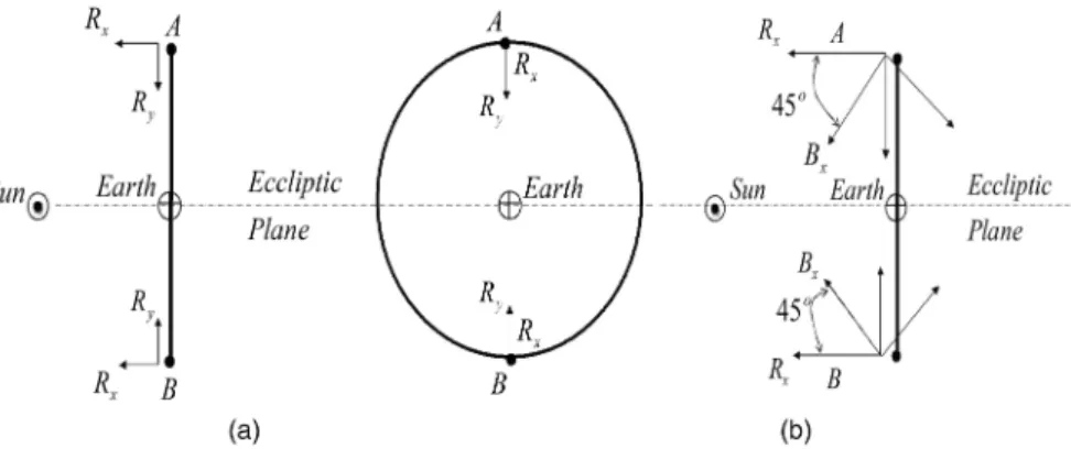
t_k and notice that both frames can themselves be rotating with respect to an inertial frame. The relative attitude of_B with respect to_Ris thus constantly zero. Assume that, at t₀, two LOS vectors ¯v₁, ¯v₂are available and that they coincide with the axes_Rx and

Fig. 1. Sun-pointing/nadir-pointing LEO satellite. Attitude with respect to trajectory frame. (a) Zero attitude. (b) 45± attitude.

Ry. Clearly, we have

b₁=r₁= [1, 0, 0]T, b₂=r₂= [0, 1, 0]T:

From (15), the K-matrix that is computed using these LOS vectors is then (with unit weighting coefficients):

K(t₀) = 2 6 6 6 4 ¢ ¢ ¢ ¢ ¢ ¢ ¢ ¢ ¢ ¢ ¡2 _¢ ¢ ¢ ¢ 2 3 7 7 7 5 (20)

where the dots in (20) represent zeros. Equation (20) shows the true values of the 16 state variables att₀. Next, assume that att₁, the second LOS vector is not available and that a third LOS vector ¯v₃ can be acquired, which lies along the axis_Rz, such that

b₃=r₃= [0, 0, 1]T:

Then, using (r₁,r₃) in (15) yields the following K-matrix: K(t₁) = 2 6 6 6 4 ¢ ¢ ¢ ¢ ¢ ¡2 _{¢ ¢} ¢ ¢ ¢ ¢ ¢ ¢ ¢ 2 3 7 7 7 5: (21)

Equation (21) shows the values of the state variables att₁. Clearly, (20) and (21) are inconsistent: although the attitude has not changed fromt₀tot₁, the state variables assume different numerical values, which depend on the values of thers used. Thus, choosing thers to be identical att₀and t₁allows for the K-matrix to consistently define a representation of the attitude of_Bwith respect to_R.

2) Although thers are required to be constant, the observed LOS vectors are not constrained to be the same physical directions at all times. This is illustrated by the following example. Consider the case of a Sun-pointing and Earth-pointing (nadir) low Earth orbit (LEO) satellite. The reference frame is defined as the trajectory frame, i.e., with_Rx pointing normal to the orbit plane,_Ry coinciding with the local nadir, and_Rz pointing forward along the in-track orbit tangent. These LEO satellites orbits are usually

Sun-synchronous, with inclinations close or equal to 90±, which avoids Sun eclipses. See the illustration in Fig. 1 for a 90± inclination. Due to the very high ratio between the Sun—SC and the Earth—SC distances (around 104), the axis_Rx can be identified with the Sun—SC LOS vector, for all practical purposes. This first LOS vector can be observed via Sun sensors. The nadir (the_Ry axis) provides a second LOS vector and can be observed by Earth sensors. Thus, thanks to this choice of the reference frame, we are in the case discussed in 2 above, where:

r₁= [1, 0, 0]T, r₂= [0, 1, 0]T:

In the case of a zero attitude, the body frame

coincides with the reference frame (see Fig. 1(a)), and the time-invariant state matrix is thus obtained from (20), i.e., X= 2 6 6 6 4 ¢ ¢ ¢ ¢ ¢ ¢ ¢ ¢ ¢ ¢ ¡2 _¢ ¢ ¢ ¢ 2 3 7 7 7 5: (22)

The above example illustrates an operational configuration where the two observed LOS vectors keep the same projections in the reference frame at all sampling times. Nonetheless, the nadir-LOS vector is continuously changing with respect to the inertial frame.

3) We now show how to relax the requirement for the body frame to be fixed with respect to the reference frame. Assume that _B(k) rotates with respect to the reference frame_Rwith an angular velocity!_k

and that!_k is known along the axes of_B(k). For the sake of illustration, consider a roll-only motion, i.e.,_B rotates around its axis_Bz, the in-track orbit tangential axis, with a magnitude of¼=4 rad/s, such that:

!_k= [0, 0,¼=4]T: (23)

This may arise from a requirement of scanning or tracking of a body-mounted camera. Assume that at t₀,_Band_Rcoincide, such that, according to the previous computations, X(t₀) is obtained from (22). Using !_k, the matrixX can be propagated fromt₀to

t₁=t₀+ 1 [8]. Considering the present example, the computations are X(t₁) =©X(t_o)©T = 2 6 6 6 4 ¢ ¢ ¢ ¢ ¢ ¢ ¢ ¢ ¢ ¢ ¡p2 p2 ¢ ¢ p2 p2 3 7 7 7 5 (24) where ©= exp 8 > > > > > > > > < > > > > > > > > : 1 2 2 6 6 6 6 6 6 6 6 4 ¢ ¼₄ ¢ ¢ ¡¼₄ ¢ ¢ ¢ ¢ ¢ ¢ ¼₄ ¢ ¢ ¡¼ 4 ¢ 3 7 7 7 7 7 7 7 7 5 9 > > > > > > > > = > > > > > > > > ; : (25)

Equation (24) provides the true value of the state matrix that represents the attitude of_B(t₁) with respect to_R. This can be visualized in Fig. 1(b). The dynamical model where!_k is measured with noises is described in the next subsection. To conclude, the proposed approach can handle time-varying attitudes, provided that a measurement of the angular velocity of_Bwith respect to_Ris available.1

Mission Architectures: Following are various and important examples of real missions architectures in which the proposed approach can be successfully implemented.

1) Consider a LEO SC whose attitude is

simultaneously stabilized with respect to the Sun—SC LOS vector (for power production via the solar arrays) and to the SC—nadir LOS vector (for Earth observation). We have already used this architecture for previous illustration (see Fig. 1). The knowledge of the relative position of the SC with respect to the Sun/Earth in some reference frame (from navigation computations) and in the body frame (from on-board measurements) allows for AD and this fits the framework proposed in this work. In the NASA LANDSAT [20] mission, the Landsat 7 satellite is designed for a Sun-synchronous, Earth mapping orbit. Its payload is a single nadir-pointing instrument and power is provided by a single Sun-tracking solar array. The satellite attitude control must maintain the SC platform within 0.015 deg of Earth pointing. In the NASA SAMPEX [21] mission, SAMPEX is a momentum-biased, Sun-pointing SC that maintains the experiment-view axis in a zenith direction as much as possible. It points its solar array at the Sun by aiming the momentum vector toward the Sun and rotating the SC one revolution per orbit about the Sun—SC axis. A two-axis digital Sun sensor and a set of five 1_{Notice that body-mounted gyros provide the inertial angular} velocity of_B. However, knowing the inertial angular velocity of_R allows us to compute the sought angular velocity!_k.

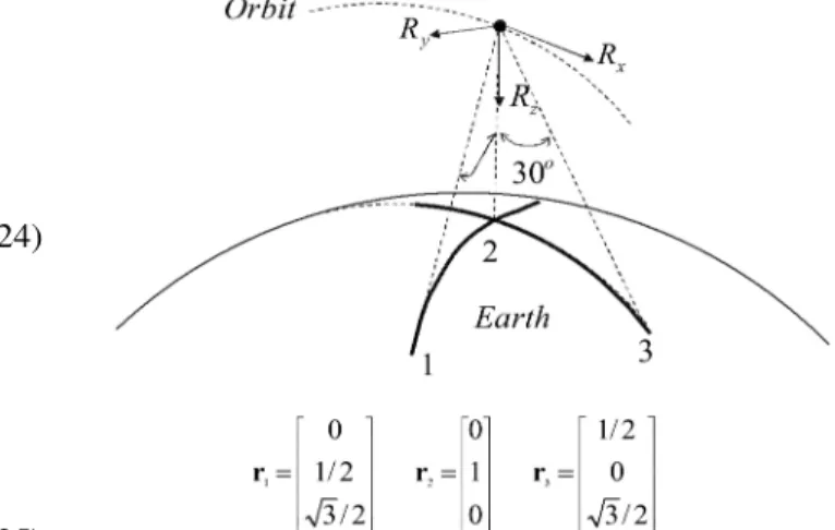
Fig. 2. LEO satellite. Attitude with respect to trajectory frame.

coarse Sun sensors are used for AD, which provides the quasi antinadir pointed attitude required by the science experience.

Consider also another architecture of LEO SC mission, e.g., a SC monitoring the Earth surface via some imaging sensor and equipped with an Earth sensor. Figure 2 illustrates a configuration of three observed LOS vectors, which are the nadir (aligned with the_Rz-axis), and two additional LOS vectors inclined by 30± with respect to the nadir in the in-track plane and in the off-track plane, respectively. The corresponding values of thers that appear in Fig. 2 are given in the trajectory frame (_Rx,_Ry,_Rz). Therefore, the proposed approach can be successfully applied provided that the Earth imaging sensor is continuously observing these three LOS vectors.

2) Consider the case of a geostationary SC. Once stabilized along the nadir, the SC is able to observe the same locations on the Earth surface all the time. Not only two of them but as many as the field of view allows for. On a geosynchronous orbit (approximately 36000 km), the SC sees the Earth with an angle of about 22 deg (assuming an Earth radius of 6400 km). Within that field of view, any digital camera can track many locations on Earth. The NASA GOES mission features a range of geostationary satellites. Figure 3 visualizes the configuration of three sensed LOS vectors, namely, the nadir, and two additional LOS vectors inclined by 10± with respect to the nadir in the in-track plane. The values of the LOS vectors’ projections in the reference frame are given in Fig. 3 for this specific configuration.

3) Consider an SC whose attitude is inertially stabilized with respect to some celestial coordinate frame. Although rotating about some equilibrium position, the SC is assumed to be stabilized enough such that the same physical directions can be observed at any time. These can be directions to stars and in that case their inertial projections are close to be time-invariant. Notice that 3-D stabilization is not needed but that even spin stabilized SC are adequate, provided that their sensors are oriented along the

Fig. 3. Geostationary satellite. Attitude with respect to trajectory frame.

Fig. 4. WMAP-Wilkison maximum anisotropy probe atL₂ Lagrangian point. Attitude with respect to Sun rotating frame.

directions of the inertially stabilized axes. In the NASA MAP [22] mission, the MAP SC is stabilized about theL2 Lagrange point, scanning the celestial sphere around the anti Sun—nadir direction. MAP spins every 2 min and its spin axis maintains a fixed angle of 22.5 deg to the Sun—Earth line. The spin axis moves around the Sun—Earth line. The SC uses Sun sensors, star trackers, and gyroscopes for AD. Figure 4 illustrates the case for two sensed LOS vectors, e.g., the Sun—SC LOS vector and the direction to a star perpendicular to it, and provides the values of thers.

Process Equation

As shown in [9] the dynamics of the true K-matrix can be modeled by the following first-order stochastic linear matrix equation

X_k+1=©_kX_k©T_k+W_k (26) whereX_k denotes the ideal noise-free K-matrix at timet_k and©_k is computed using the angular velocity vector!_k (as measured by a triad of body-mounted gyroscopes during a small time increment¢t), i.e.,

−_k=1 2 · ¡[!_k£] !_k ¡!T k 0 ¸ (27) ©_k= exp_f−_k¢t_g (28)

where, in (27), [!_k£] denotes the cross-product matrix which is defined by the identity!_k£u= [!_k£]ufor any vectoru₂R3_{. One can see that (26) is a special}

case of the general process equation described in (1), and is, therefore, implementable in an MKF. As shown in Appendix I, the matrixW_k can be expressed as follows

W_k= (X_{kEk¡ Ek}X_k)¢t (29) whereX_k is the state matrix att_k, the time increment is denoted by¢t, and_Ek is the following 4_£4 skew-symmetric matrix Ek= 1 2 · ¡[²_k£] ²_k ¡²T k 0 ¸ (30) The 3_£1 vector²_k denotes the additive error in the measured value of the body angular velocity. In this work we consider the special case where ²_k is a zero-mean white noise process with covariance matrix

Q²

k=¢t. Moreover, it is assumed that²k is uncorrelated

with the initial state,X₀. Using these assumptions it can easily be shown that the matrix noiseW_k is a zero-mean process.

State-Dependent Process Noise: Taking advantage of the bilinear structure ofW_k with respect to²_k and to

X_k, we seek an analytic expression for its covariance matrixQ_k. Previous works on Kalman filtering with this type of noise state-dependence can be found in [14]—[16].

PROPOSITION1 Let_fe₁,e₂,e_3gdenote the three columns of the identity matrixI₃inR3_{. LetM and¡}

k

denote the following16_£3 and16_£16 matrices:

MT= [_¡[e_1£] _¡e_{1 ¡}[e_2£] _¡e₂

¡[e_3£] _¡e₃ I₃ 0] (31)

¡_k=1₂[(I₄₋X_k)_¡(X_kT₋I₄)]M: (32)

Then,

i) The16_£16covariance matrix ofW_k, denoted by

Q_k, satisfies:

Q_k=E_f¡_k²_k²T_k¡_kT_g¢t2: (33)

ii) If, furthermore, the components of²_k are independent and identically distributed with covariance parameter¾2=¢t, andN_kdenotes the second-order moment of the stateX_k, thenQ_k is computed as follows: Q_k= 3 X i=1 ¨_iN_k¨_iT¾2¢t (34) where fori= 1, 2, 3 ¨_i=1₂(A_i©A_i) (35)

with_©denoting the Kronecker sum[24]and A₁= · _{0 ¡e} 3 e2 e1 ¡1 0 0 0 ¸ A₂= ·_e 3 ¡0 ¡e1 e2 0 _¡1 0 0 ¸ A₃= ·_¡e 2 e1 0 e3 0 0 _¡1 0 ¸ : (36)

The proof is provided in Appendix II. The usefulness and implementation of both results from Proposition 1 is discussed in the next section.

Measurement Equation

The measurement model equation is the following simple matrix equation [9]

Y_k+1=X_k+1+V_k+1 (37) whereY_k+1 is the measured K-matrix constructed using the noisy vector observations acquired at timet_k+1, andV_k+1denotes the measurement noise. Looking at the general measurement model described in (2) one realizes that (37) is a particular case of (2) whereHs

k+1=Gsk+1=I4andº= 1. Thus (37) is

readily implementable in the MKF.

Given a batch of vector observations,b_i,r_i,i= 1, 2,: : :,m (m >1), acquired att_k+1, the expression for the noise matrixV_k+1in the measurement equation (37) is V_k+1= m X i=1 ®_iV_k+1i (38)

where®_i=¢a_i=PM_i=1a_i, and thea_is are positive weighting scalars associated with each vector measurement. Each matrixVi

k+1in (38) is expressed

using a pair,±b_i(t_k+1),r_i(t_k+1) as follows,

V_k+1= ·_S b¡·bI3 zb zT b ·b ¸ (39) where B_b=±b_k+1rT k+1, Sb=Bb+BbT z_b=±b_k+1£r_k+1, ·_b= tr(B_b) (40) and where the 3_£1 vector±b_i(t_k+1) is the error in the

ith vector observation. It is assumed that the sequence

±b_i(t_k+1),k= 1,: : :,m, is a zero-mean, white sequence with a known covariance matrix,Rbi

k+1. Moreover,

the vector observations acquired at the same time are assumed to be uncorrelated with one another. That is,

E_f±b_i(t_k+1)_g=0 (41a)

E_f±b_i(t_k+1)±b_i(t_l)T_g=Rbi

k+1±k+1,l (41b) E_f±b_i(t_k+1)±b_j(t_k+1)T_g=Rbi

k+1±ij (41c)

wherei,j= 1, 2,: : : m,k,l= 1, 2: : :and±_k+1,l,±_ij denote Kronecker deltas. In addition, it is assumed that the vector observations are uncorrelated with the process noise²_k and with the initial state X₀. From (39) and (40) it appears that the elements ofVi

k+1

are linear combinations of the elements of±b_i(t_k+1). Since±b_i(t_k+1) is zero-mean, then the sequenceVi

k+1

is also zero-mean. Since V_k+1is a weighted sum of zero-mean sequencesVi

k+1(see (38)), thenVk+1 is

also zero-mean. Using (41) an analytic expression for the covariance matrix ofV_k+1, denoted byR_k+1, can be derived. A summary of the computation of the 16_£16 matrixR_k+1is given next. Its proof is lengthy but straightforward and is provided in Appendix III. For the sake of clarity the symbolt_k+1 is dropped from the following equations; however, it should be remembered that all the computations carry the time tag t_k+1. Givenr_i,Rbi_{, anda}

i,i= 1, 2,: : : m, compute ˜ R_i= ·_[r i£] ri ¡rT i 0 ¸ (42a) ¤_i= ( ˜R_i−I₄)M (42b) R_i=¤_iRbi_¤ i T _(42c) ®_i=Pmai i=1ai (42d) R_k+1= m X i=1 ®2_iR_i (42e)

where the matrix Mis defined in (31).

FILTER IMPLEMENTATION State-Dependent Process Noise

1) As mentioned earlier, and as seen from (29), the process noiseW_k is a function of the state X_k. Fortunately, this dependence is linear which allows an exact computation of the covariance ofW_k provided that the second-order moment of X_k,N_k, is known. It is well known thatN_k can be propagated via a Lyapunov difference equation. The computation of

Q_k is thus done as follows:

Q_k= 3 X i=1 ¨_iN_k¨_iT¾2¢t (43a) Fk=©k−©k (43b) N_k+1=_FkN_kFkT+Q_k (43c)

where the matrices¨_iare defined in (35) and (36). The above equations are implemented in the time-propagation stage of the Kalman filter.

2) While the above algorithm for computing

Q_k has the merit of being exact, it implies an additional computational burden in the filter, which should be weighed against the performance improvements. On the other hand, the practitioner

may consider implementing the following approximate computations. In order to avoid computing the matrix

N_k,Q_k can be approximated by simply replacing the stateX_k by its best available estimate, ˆX_k=k, in (32), (33). This step is similar to what is done in an extended Kalman filter (EKF). Then, assuming independent and identically distributed components in²_k, a first-order approximation in¢tfor the covariance matrix ofW_k yields

Q_k'1₄[(I₄₋Xˆ_k=k)_¡( ˆX_k=kT ₋I₄)]MMT

£[(I₄₋Xˆ_k=k)_¡( ˆXT

k=k−I4)]T¾2¢t:

3) A third option for approximatingQ_k is

Q_k= ¯Q_k−I₄: (44) Under additional conditions, (44) provides a drastic reduction in the covariance computation while maintaining satisfactory performance. This case is discussed in the subsection on reduced covariance.

Singularity of the Measurement Noise Covariance Matrix

The covariance matricesR_i as computed in (42c) are singular. Indeed, assuming that the covariance matrix in each vector-measurement errorRbi _{is of full}

rank (rank three), then every 16_£16 matrixR_i is at most of rank three, and is, thus, singular. Therefore, if there is a single vector measurement (m= 1) at

t_k+1the rank ofR_k+1is three andR_k+1is singular. Simulations showed that if two noncollinear vector observations are acquired att_k+1, the rank of R_k+1

increases to six, and, in the case of three or more than three noncollinear measurements (m_¸3), the rank equals nine. This is consistent with the properties of the error matrixV_k+1 (see (37)). SinceY_k+1and X_k+1

are symmetric matrices with a trace equal to zero, thenV_k+1 has necessarily the same properties. These properties introduce seven linear constraints among the elements ofV_k+1; namely, six constraints for the symmetry and one for the trace, which lowers the rank ofV_k+1from 16 down to 9. There are several techniques to cope with the issue of a singular

measurement covariance matrix (see e.g. [10, p. 354]). To circumvent the problem here, we add small values to the main diagonal ofR_k+1, which has a stabilizing effect on the numerics of the Kalman filter. This is done by choosing a small¯ relatively to the assumed level of the noise, and computingR_k+1 as follows

R_k+1=

m X

i=1

®2_iR_i+¯I₁₆ (45) whereI₁₆ denotes the 16_£16 identity matrix.

Algorithm Summary

The MKF of the K-matrix is summarized in the following. 1) Initialization: ˆ X₀₌₀=Y₀, P₀₌₀=R₀: (46) 2) Time Update: ˆ X_k+1=k=©_kXˆ_k=k©T_k (47) Fk=©k−©k (48) P_k+1=k=_FkP_k=kFkT+Q_k: (49) 3) Measurement Update: ˜ Y_k+1=Y_k+1¡Xˆ_k+1=k (50) S_k+1=P_k+1=k+R_k+1 (51) K_k+1=P_k+1=kS¡_k+11 (52) ˆ X_k+1=k+1= ˆX_k+1=k+ 4 X j=1 4 X l=1 K_k+1jl Y˜_k+1Elj (53)

whereK_k+1jl is a 4_£4 submatrix of the 16_£16 matrix

K_k+1defined by K_k+1= 2 6 6 4 K11 k+1 ¢¢¢ Kk+114 .. . . .. ... K41 k+1 ¢¢¢ Kk+144 3 7 7 5 | {z } 4 submatrices 9 > = > ; 4 submatrices (54) P_k+1=k+1= (I_16¡K_k+1)P_k+1=k(I_16¡K_k+1)T +K_k+1R_k+1K_k+1T : (55)

The MKF that is described in (46)—(55) produces a sequence of K-matrix estimates ˆX_k=k. This constitutes the first stage of the attitude estimation process. The second stage consists of the computation of the eigenvector of ˆX_k=k that belongs to the largest eigenvalue.

Reduced Covariance Filter

In this section we show how to reduce the computational complexity of the filter by making further reasonable assumptions on the statistics of the system’s noises. Namely, we assume that the rows of W_k are independently identically distributed with 4_£4 covariance matrix ¯Q_k. Similar assumptions are made with respect to the matrixV_k and to the initial estimation error matrix ¢X₀₌₀. These assumptions are expressed as

Q_k= ¯Q_k−I₄ (56a)

R_k= ¯R_k−I₄ (56b)

P₀₌₀= ¯P₀₌₀₋I₄: (56c)

As shown in Appendix IV, the use of (56) in the equations of the filter ((46)—(55)) reduces the

covariance computation from 16_£16 to 4_£4 matrix equations. Moreover, it enables a more compact notation in the state measurement update stage. The reduced covariance filter is summarized next.

1) Initialization: ˆ X₀₌₀=Y₀, P¯₀₌₀= ¯R₀: (57) 2) Time Update: ˆ X_k+1=k=©_kXˆ_k=k©T_k (58) ¯ P_k+1=k=©_kP¯_k=k©T_k+ ¯Q_k (59) where ¯P_k=k and ¯P_k+1=k are 4_£4 matrices.

3) Measurement Update: ˜ Y_k+1=Y_k+1¡Xˆ_k+1=k (60) ¯ S_k+1= ¯P_k+1=k+ ¯R_k+1 (61) ¯ K_k+1= ¯P_k+1=k( ¯S_k+1)¡1 (62) ˆ X_k+1=k+1= ˆX_k+1=k+ ˜Y_k+1K¯_k+1T (63) ¯ P_k+1=k+1= (I_4¡K¯_k+1) ¯P_k+1=k(I_4¡K¯_k+1)T + ¯K_k+1R¯_k+1K¯_k+1T (64) where ¯P_k+1=k+1, ¯S_k+1, and ¯K_k+1 are 4_£4 matrices. As a result of assumptions (56) the filter covariance computations are identical for each 1_£4 row of the estimation error matrix. This is why a single 4_£4 covariance computation is needed. If the full covariance matrices are needed they are readily computed as shown in Appendix IV by

P_k=k= ¯P_k=k−I₄ (65a)

P_k+1=k= ¯P_k+1=k−I₄ (65b)

S_k+1= ¯S_k+1−I₄ (65c)

Kk+1= ¯Kk+1−I4: (65d)

Covariance Matrix of the Quaternion Estimation Error

In this section we use and extend a previous result, as presented in [3] in order to evaluate the covariance matrix of the quaternion estimation error. It is shown how this matrix can be extracted from the covariance matrixP_k=k, as computed in (55).

Let±zdenote the measurement error in the 3_£1 vectorzof a measured K-matrix, which is constructed frommvector measurements and let P_zz denote the covariance matrix of±z. Let±qdenote the quaternion multiplicative estimation error; that is

±q= ˆq?q¡1 ₍₆₆₎

whereqis the true quaternion, ˆqis the estimate,?

and ˆq¡1_{denote the operations of quaternion product}

and quaternion inverse, respectively [1, p. 758]. Thus,

±qitself is a quaternion; it has a vector part ±eand a scalar part±q. This error-quaternion is related to the rotation that brings the true body frame onto the estimated body frame. Assuming that the angle of this rotation is small,±qis approximated by 1, as done in [3]. The uncertainty is thus concentrated in±e. It can be shown [3] that a good approximationP_eeto the covariance matrix of±eis computed as

P_ee=NP_zzN (67) where N= ( 2 m X i=1 ®_i(I_3¡r_irT i) )¡1 (68) andr_i,i= 1, 2,: : :,m, is the batch of observed LOS vectors, as resolved in the reference frame, which are acquired at a particular epoch time. In order to use (67) and (68) in our algorithm, consider±zas an estimation error rather than a measurement error. The 3_£3 covariance matrix of±z,P_zz, is easily extracted from the 16_£16 covariance matrixP_k=k. Since

±z= 2 6 4 ¢X(1, 4) ¢X(2, 4) ¢X(3, 4) 3 7 5 (69)

then, using (14) withm= 4 andn= 1, yields

P_zz= 2 6 4 P(13, 13) P(13, 14) P(13, 15) P(14, 13) P(14, 14) P(14, 15) P(15, 13) P(15, 14) P(15, 15) 3 7 5 (70) whereP(13, 13) denotes the element ofP_k=k at location (13, 13). Thus, one can evaluate the covariance

matrixP_ee by first computingP_k=k from (55), then by extracting the submatrix P_zz (70) and finally by using (67) and (68). Notice that the matrixN in (68) only depends on the chosen reference directions. If the reference frame is inertial,N is computed only once at the start of the algorithm. OtherwiseN is propagated using the dynamics of the reference frame, which is assumed to be accurately known.

CONSTRAINED ESTIMATION

In this section a constrained estimation algorithm is developed which enforces the properties of symmetry and zero-trace on the K-matrix estimate. For this purpose, one possible approach is to develop a reduced-order model according to the number of constraints among the state variables. This would however destroy the matrix formulation of the estimator. In order to preserve the original matrix formulation, the PM approach for constrained estimation is adopted. Next, we briefly explain the main idea of the constrained estimation approach via PM measurement. Assume that the true state variable

X satisfies the following constraint

wheref(X) may be a scalar, a vector, or a matrix mapping and assume that an imaginary device measuresf(X) with some small error. The associated PM equation is thus

f(X) =v (72)

wherevis the associated PM noise with appropriate dimension. In order to fit in the Kalman filtering framework, this noise is typically modeled as a zero-mean white noise with a given covariance matrix

R_v. Based on the PM model equation (72), a PM update stage is developed in the Kalman filtering framework and sequentially implemented after a nominal unconstrained update stage. The PM noise covariance matrixR_v is used as a tuning parameter in the filter to “strengthen” or “soften” the constraint. For instance, if the value ofR_vis very low, the constraint will be strongly enforced via the PM measurement update stage. In the following, PM model equations are developed for the symmetry and trace constraints.

Notice that the constrained estimation approach via PM consists of relaxing a hard constraint in the underlying optimization problem, and varying the degree of enforcement of the constraint by changing some parameter–here the covariance of a virtual noise. Thus, what matters aboutv is only the value given to its covariance, because that value will impact the PM update stage and will thus enforce the constraint on the estimate. That technique was successfully applied, e.g., to quaternion normalization in [17] and to direction cosine matrix orthogonalization in [18]. Reference [19] presents a comprehensive survey on constrained Kalman filtering via PM (called there pseudoobservations) and projections, develops a successful combination of these approaches, and illustrates it in a constrained quaternion estimation problem.

SYMMETRY CONSTRAINT

Symmetry Pseudomeasurement: Out of the many formulations of the symmetry constraint on a matrix

X, we consider the following one:

1 2(X+X

T_{) =X: (73)}

It is assumed that an imaginary device is

measuring the 4_£4 state matrixX_k+1 with some small zero-mean white noise, denoted byV_k+1sym, and is giving as output the symmetric part of its best available estimate ˆX_k+1=k+1, where ˆX_k+1=k+1is obtained from (53). Thus, the symmetry PM equation is

1

2( ˆXk+1=k+1+ ˆXk+1=k+1T ) =Xk+1+V sym

k+1: (74)

Note that if ˆX_k+1=k+1 is error free and if we drop the matrix noiseV_k+1symfrom (73), we recover (73), which is the desired basic property. Since, as is evident from

(2), (74) has the standard structure of a linear matrix measurement, it can be incorporated into the system mathematical model. LetRsym_k+1 denote the 16_£16 covariance matrix ofV_k+1sym. Using (74) and Rsym_k+1, the symmetry-measurement update stage is formulated as

˜ Y_k+1=1₂( ˆX_k+1=k+1T _¡Xˆ_k+1=k+1) (75a) S_k+1=P_k+1=k+1+Rsym_k+1 (75b) Kk+1=Pk+1=k+1Sk+1¡1 (75c) ˆ X_k+1=k+1+ = ˆX_k+1=k+1+ 4 X j=1 4 X l=1 Kjlk+1Y˜k+1Elj (75d) P_k+1=k+1+ = (I_{16¡ Kk+1})P_k+1=k+1(I_{16¡ Kk+1})T +_Kk+1R_k+1sym_Kk+1T (75e)

where the 4_£4 matrices_Kjl_k+1 in (75d) are submatrices of the 16_£16 matrix_Kk+1; they are defined according to the partition described in (54). The covariance matrixR_k+1symis a filter tuning matrix parameter, according to which one can weight the symmetry constraint in the estimation process. For example, takingRsym_k+1 to zero yields a unity gain matrix, i.e.,_Kk+1=I₁₆, which then produces the following update stage:

ˆ

X_k+1=k+1+ =1₂( ˆX_k+1=k+1+ ˆX_k+1=k+1T ): (76) In that case the symmetry update stage (76) produces the symmetric part of the previous estimate. This intuitively appealing result can also be drawn from a deterministic optimization approach; indeed, it can be shown that the symmetric part of any square matrix is its closest symmetric matrix (with respect to the Frobenius norm [25]). More generally, the latter result can be seen as a particular case of a recursive least-squares estimate converging to an orthogonal projection estimate for a vanishingly small variance parameter (see [19] for a discussion between these two approaches).

Trace Constraint

The trace constraint is handled using the following PM model:

0 = trX_k+1+v_k+1tr (77)

where “tr” denotes the trace operator,vtr

k+1is a scalar

zero-mean white noise with covariancertr

k+1, and the

value of the PM is 0. Using the definition of the trace operator trX_k+1= 4 X i=1 X_k+1(i,i) = 4 X i=1 e_iTX_k+1e_i (78)

wheree_i,i= 1, 2, 3, 4, are the standard unit vectors in

R4_{. Equation (78) has the standard form of a linear}

matrix measurement model. Using (78) the trace update stage is formulated as follows

htr= 4 X i=1 (e_i−e_i) (79a) s_k+1=htrTP_k+1=k+1htr+r_k+1tr (79b) k_k+1=P_k+1=k+1htr=s_k+1 (79c) ¯ K_k+1= 4 X j=1 kj_k+1e_jT (79d) ˆ X_k+1=k+1+ = ˆX_k+1=k+1¡(tr ˆX_k+1=k+1) ¯K_k+1 (79e) P_k+1=k+1+ = (I_16¡k_k+1htrT )P_k+1=k+1(I_16¡k_k+1htrT )T +r_k+1tr k_k+1kT_k+1 (79f)

where each vectorkj_k+1in the computation of ¯K_k+1

(79d) is the 4_£1 column-vector at position j,j= 1, 2, 3, 4, in the 16_£1 gain column-vector,k_k+1. Equation (79e) is proved as follows:

ˆ X_k+1=k+1+ = ˆX_k+1=k+1+ 4 X j=1 [(_¡tr ˆX_k+1=k+1)(kj_k+1e_jT_)] = ˆX_k+1=k+1¡(tr ˆX_k+1=k+1) 0 @ 4 X j=1 kj_k+1e_jT 1 A = ˆX_k+1=k+1¡(tr ˆX_k+1=k+1) ¯K_k+1: (80) The first equality in (80) is the general formulation of the state measurement update stage in an MKF. The second equality stems from the fact that tr ˆX_k+1=k+1

is independent ofj, and the last equality is obtained by using (79d). Similar to the symmetry constraint case, the covariancertr

k+1is used as a tuning parameter

in order to enforce the zero-trace property along the estimation process. In the limiting case where

r_k+1tr = 0, straightforward computations yield ¯

K_k+1=1

4I4: (81)

Using (81) into (79e) yields ˆ

X_k+1=k+1+ = ˆX_k+1=k+1¡1

4(tr ˆXk+1=k+1)I4: (82)

Computing the trace of ˆX_k+1=k+1, as given in (82), and using the fact that trI₄= 4, yields tr ˆX_k+1=k+1= 0; that is, the updated ˆX_k+1=k+1 exactly satisfies the zero-trace constraint.

The constrained MKF consists of the algorithm described earlier, (46)—(55), to which the symmetry and trace update stages are added. Thus, each update stage operates on the preceding state estimate and

estimation-error covariance. Like in an iterative Kalman filter, the three stages are performed sequentially at the same epoch time.

NUMERICAL STUDY

In this section the unconstrained MKF, the constrained MKF (CMKF) and the

Optimal-REQUEST (OPREQ) filter [9] are tested and compared via extensive Monte-Carlo simulations. In the present case study we consider an SC with the same kinematics model as the Microwave Anisotropy Probe (MAP) satellite [22], which was launched on June 30, 2001. The attitude measurement devices simulated here are composed of a digital Sun sensor (DSS), an autonomous star-tracker (AST), and a triad of rate gyroscopes. Two Cartesian coordinate frames are considered; namely, the Sun frame, which is assumed to be inertial, and the body frame. The rotation of the body frame with respect to the Sun frame is composed of a spin rotation and of a nutation; the spin and the nutation rates are 0.464 rev/min and 1 rev/hr, respectively; the constant nutation angle, which is defined between the SC spinning axis and the anti-Sun LOS vector, is equal to 22.5 deg.

It is assumed that the AST observes the same star during the whole simulation. Therefore, two identical inertial LOS vectors are observed at each sampling time; namely, the Sun—SC LOS vector, and the star—SC LOS vector. These LOS vectors are represented in the Sun frame by the unit vectorsr₁

andr₂, respectively. The Sun frame is assumed to have its third axis coinciding with the LOS between the SC and the Sun, thusr₁= [0 0 1]T. For the sake of the example, it is assumed that the AST can find a star along a direction perpendicular tor₁, for instance,

r₂= [1 0 0]T_{. The unit vector measurements,b} i, i= 1, 2, are simulated by adding a small zero-mean white Gaussian noise to the ideal observed directions, and by normalizing the result; that is

b_i= Ari+±bi

kAr_i+±b_ik (83)

whereAis the correct transformation matrix from the Sun to the body coordinates and

±b_{i» N f}0,¾_i2I_3g (84) fori= 1, 2. Here,¾₁ equals 1 arc-mn (_'17 mdeg), and¾₂equals 10 arc-sec (_'2:8 mdeg). The vector measurement sampling period is 10 s. The output of a triad of gyroscopes is contaminated by a zero-mean Gaussian white noise with a covariance matrix

¾2

²I3, where¾²= 100 mdeg/hr. The gyros sampling

period is 0.5 s. It is assumed that the initial attitude is completely unknown. Each simulation run lasts 10000 s.

Comparison between Optimal-REQUEST and the MKF

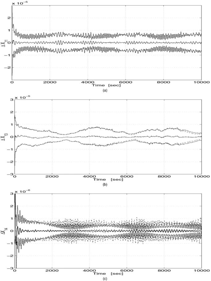
The results of the Monte-Carlo simulation (100 runs) are summarized in Figs. 5—8. In each figure the solid lines are used to plot the variables of the unconstrained MKF, that is, the full covariance filter as described in (46)—(55). The dashed lines are associated with the OPREQ variables. Let¢X₁₁,

¢X₁₃, and¢X₁₄ denote the elements (1, 1), (1, 3), and (1, 4), respectively, of the updated estimation error matrix¢X_k=k. Extensive simulations show that the behavior of these three elements represents the behavior of all other elements of the matrix¢X_k=k. Figure 5 shows the time history of the means and of the_§1¾-envelopes of ¢X₁₁,¢X₁₃, and¢X₁₄. Figure 5(a) shows that the plots of¢X₁₁OPREQ and

¢XMKF

11 are practically undistinguishable. The means

oscillate around zero with two time periods; namely, a short period of about 2 min, which corresponds to the spin rotation of the SC, and a long period of 1 hr, which is due to the SC nutation. The order of magnitude of the standard deviations is 5_£10¡6_.

Figure 5(b) shows that, similar to¢X₁₁, the filters OPREQ and MKF yield very close variations in

¢X₁₃. However, the oscillations in¢X₁₃ are less sensitive to the short period than in¢X₁₁. In Fig. 5(c), however, we notice that the oscillations in the

mean of¢X₁₄OPREQare much less damped than the oscillations in the mean of¢XMKF

14 , and the ratio

between the amplitudes of those oscillations reaches 8. Furthermore, the_§1¾-envelope of¢XMKF

14 constitutes

a lower-bound for that of¢X₁₄OPREQ. The dc level of the oscillations in the standard deviation is about 4_£10¡7_{for the MKF, and twice as large (8£10}¡7₎

for OPREQ. Thus, forX₁₄, MKF clearly outperforms OPREQ. The advantage of MKF becomes even more obvious when analyzing the angular and quaternion estimation errors.

Next, the gains of MKF and OPREQ are compared. For this purpose we compute the scalar

½_MKF as the Euclidean norm of the 16_£16 gain matrix_Kk+1of MKF, and plot its Monte-Carlo mean versus the mean of the gain of OPREQ½_OPREQ. Figure 6 shows the variations of the Monte-Carlo means of½_MKF (solid) and of½_OPREQ(dashed). During the transition phase, the first 1500 s, the two quantities are very close to one another. Then½_MKF

reaches a steady-state value around 0.015, while

½_OPREQ oscillates at the spin and nutation frequencies. The maxima of½_OPREQ are about 0.025 and the dc level of the oscillations is around 0.020. This result gives some insight into the result described earlier in Fig. 5(c); because of the higher gain, OPREQ filter weighs the new incoming observations more heavily than MKF; therefore, the update estimate in OPREQ is noisier than that in the MKF.

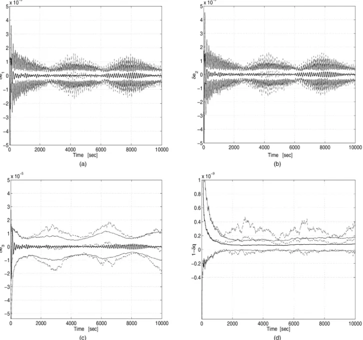
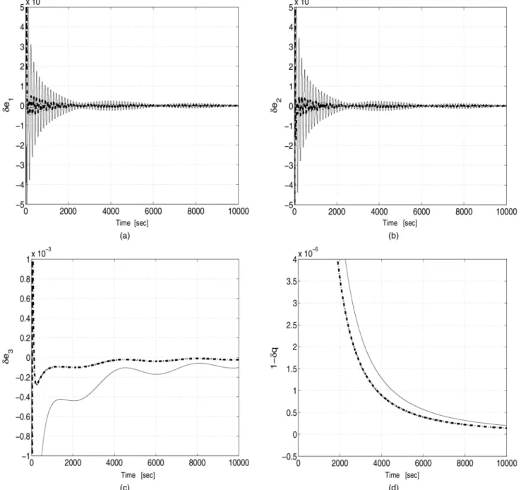
As mentioned earlier the quaternion estimation error, denoted by±q, is defined as the quaternion of the small rotation that brings the estimated body frame onto the true body frame (see (66)). It has four components, which are denoted by±e₁,

±e₂,±e₃, and±q. The variations of the means and §1¾-envelopes of the four components of±qare depicted in Fig. 7. As can be seen from Figs. 7(a) and (b), the errors±e₁ and±e₂have very similar variations. The oscillations in the means are less damped in OPREQ than in the MKF; the ratio between the oscillation peaks reaches 8. The dc level of the_§1¾-envelopes in OPREQ is twice that of the MKF (1:2_£10¡5_{as compared with 6£10}¡6_).

The same analysis applies to±e₃in Fig. 7(c) except that the variations of ±eOPREQ₃ are much noisier. As opposed to±eOPREQ₃ , the variations of±eMKF

3 have

a regular oscillating pattern, essentially modulated by the nutation frequency. Instead of plotting the variations of±q, we plot those of (1_¡±q) in Fig. 7(d); indeed, this quantity is the one that becomes small when the quaternion estimation error becomes small (a quaternion expressing a zero-rotation is equal to [0 0 0 1]T_{). After a transition phase of about 1500 s,}

the plots of OPREQ and the MKF clearly separate. The variations of 1_¡±qMKF _{are smooth, with a mean}

of 10¡10 _{and a standard deviation of 10}¡10_{; on the}

other hand, the mean of 1_¡±qMKF _{oscillates above}

10¡10_{, and the standard deviation is of the order of}

2_£10¡10_.

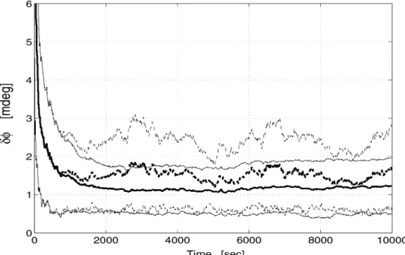
Let±Ádenote the angle of the small rotation that is represented by ±q. This angle is extracted from ±qusing the known relation,±q= cos(±Á=2). Figure 8 presents the time histories of the mean and of the_§1¾-envelope of±Á. The mean of the MKF is stabilized at 1.2 mdeg, while the mean of OPREQ oscillates above it, around a dc level of 1.7 mdeg, i.e., the mean error of OPREQ is about 1.4 times larger than that of MKF. The standard deviation in the MKF is about 0.8 mdeg, about 1.5 times smaller than that in OPREQ, which is 1.2 mdeg.

Overall, we see that MKF outperforms OPREQ. We also deduce from Fig. 7(d) that there is a small bias in the estimated quaternion. Considering the order of magnitude in±Á, both algorithms perform well since the estimation angular error is at a level of 1.2 mdeg (in MKF) and of 1.7 mdeg (in OPREQ), which is less than the measurement angular errors, i.e., about 3 mdeg in the most accurate measurements, and about 17 mdeg in the least accurate ones.

Discussion

We saw in Fig. 5(c) that the Monte-Carlo standard deviation (Monte-Carlo STD) in¢X₁₄ were twice as large in OPREQ as in MKF; the same ratio in favor of MKF appeared in Figs. 7(a) and (b) with respect to the Monte-Carlo STD in±e₁ and±e₂. Fig.7(c)

Fig. 5. Monte-Carlo means and §1¾ envelopes of the estimation errors¢X₁₁,¢X₁₃and¢X₁₄ in MKF (solid) and in the OPREQ filter (dashed). (a)¢X₁₁. (b)¢X₁₃. (c)¢X₁₄.

features a ratio of 1:5 between the Monte-Carlo STD of±e₃ in OPREQ and MKF. The ratio between the Monte-Carlo STD (and means) of±qin OPREQ

and MKF is also 1.5, according to Fig. 7(d). Finally, Fig. 8 shows a ratio of 1.4 between the Monte-Carlo means of ±Áin both filters, and the same holds

Fig. 6. Monte-Carlo means of the gains½_OPREQ (dashed) and½_MKF(solid).

for the Monte-Carlo STD of±Á. We can therefore conclude from these results that the MKF algorithm outperforms the OPREQ algorithm, and that the increase in performance can be quantified by ratios between 1.4 and 2.

The present discussion is concerned with an analysis of the ratio in the performances increase. We first derive conditions under which the MKF algorithm reduces to OPREQ. Assume thatW_k,V_k, andP₀₌₀ have independent identically distributed rows with 4_£4 covariance matrices, ¯Q_k, ¯R_k, and ¯P₀₌₀, respectively.2 _{In addition, assume that the gain matrix}

in (52),_Kk+1, is a scalar matrix, i.e.,

Kk+1=½k+1I16 (85)

then the filter update equations (52) and (53) become ˆ

X_k+1=k+1= (1_¡½_k+1) ˆX_k+1=k+½_k+1Y_k+1 (86a) ¯

P_k+1=k+1= (1_¡½_k+1)2P¯_k+1=k+½2_k+1R¯_k+1 (86b) where ˆXdenotes the estimate of the K-matrix,Y_k+1is the matrix measurement constructed using the vector measurement acquired att_k+1, ¯P denotes the 4_£4 estimation error covariance matrix for each row of the estimation error matrix, and ¯Rdenotes the covariance matrix of the effective measurement noise used in MKF. Equations (86) are obtained by using (85) in (63) and (64). The update equations in OPREQ are 2_{These assumptions lead to to the reduced covariance MKF as given} in (57)—(64).

written here for convenience [9]

K_k+1=k+1= (1_¡½¤_k+1)K_k+1=k+½¤_k+1±K_k+1 (87a)

P_k+1=k+1= (1_¡½¤_k+1)2P_k+1=k+½¤_k+12_Rk+1 (87b) whereK_k+1=k+1 denotes the updated estimate of the K-matrix,±K_k+1 is the matrix measurement at

t_k+1,½¤_k+1is the optimized fading memory factor,

P_k+1=k+1 and_Rk+1denote the “uncertainty” matrices for the updated estimation error and for the effective measurement noise used in OPREQ, respectively. Comparing (86) and (87) we realize that they have similar structures. They differ, however, because the matrices ¯P_k+1=k+1 andP_k+1=k+1 are different, and so are the matrices ¯R_k+1 and_Rk+1. In fact, these matrices are related as follows

Rk+1= 4 ¯Rk+1 (88)

P_k+1=k+1= 4 ¯P_k+1=k+1: (89) Equation (88) is easily shown by recalling the

definition of _Rk+1[9], which yields Rk+1 ¢ =E[V_k+1V_k+1T ] =E " ₄ X i=1 vc ivci T # = 4 X i=1 E[vc ivci T ] = 4 ¯R_k+1

Fig. 7. Monte-Carlo means and§1¾envelopes of the quaternion estimation errors in MKF (solid) and in OPREQ filter (dashed). (a)±e₁. (b)±e₂. (c)±e₃. (d) 1_¡±q.

wherevc

i,i= 1, 2, 3, 4, denote the 4£1 column-vectors

of the matrixV_k+1. Notice that these vectors are identical to the rows ofV_k+1sinceV_k+1 is a symmetric matrix (see (39) and (40)). The third equality is due to the linearity of the expectation operator. The last equality stems from the assumption that the rows of

V_k+1(and thus also its columns) are independent and identically distributed, with covariance matrix ¯R_k+1. The same argument is readily used forP_k+1=k+1. As a result, the covariance update equations of the MKF and of OPREQ are identical, up to a multiplication by a constant.

While finding the conditions under which the general MKF algorithm reduces to the OPREQ algorithm, we have quantified the difference between

the effective measurement noise levels in the filters, and found that it is four times greater in OPREQ than in the matrix filter. It is believed that this is the principal cause of the discrepancy between the filters’ performance. The latter is illustrated by a simple example. Consider the following scalar state-space equations

x_k+1=x_k+w_k (90)

y_k+1=x_k+1+v_k+1 (91) wherew_k andv_k+1 are the process and measurement noise sequences, respectively, which satisfy the usual stochastic assumptions of the basic state-space model. Letqand rdenote the covariances ofw_k andv_k, respectively. The scalar algebraic Riccati equation is

Fig. 8. Monte-Carlo means and §1¾ envelopes of the angular estimation error±Áin MKF (solid) and in OPREQ filter (dashed).

readily formulated as follows:

p2₁+qp_1¡qr= 0 (92) wherep₁denotes the steady-state estimation error covariance. Solving forp₁in (92) and assuming3 _that q=r_¿1 yields the following approximation for p₁:

p_1'pqr: (93)

It is clear from (93) that multiplying the measurement noise covariancer by 4 will deteriorate the estimation error standard deviationpp₁by factor ofp2_'1:4, which is close to the Monte-Carlo simulations results.

Constrained Matrix Kalman Filter

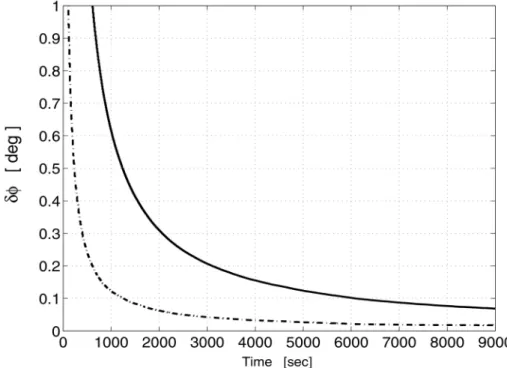
We test here the performance of the CMKF, which is the MKF that embeds the symmetry and trace update stages. We compare the response of the CMKF and the MKF to an initial perturbation in the symmetry and trace properties of the estimate matrix. The initial perturbations in the elements of the initial estimate are zero-mean uniformly distributed random variables with standard deviation¾_dst= 0:05. The covariance matrix of the symmetry PMRsym_k+1 is chosen asR_k+1sym= (¾_dst)2I₁₆, and the covariance of the trace PM isr_k+1tr =¾_dst2 . All the other simulation conditions are identical to those of the preceding simulation. The results of a 100-run Monte-Carlo simulation are presented in Figs. 9 and 10. For both MKF and CMKF, Fig. 9 shows plots of the MC-means for±Á

3_{This assumption is fully justified in the application case where} the process noise comes from gyro outputs and the measurement noise comes from vector measurement sensing devices. In this case, q_'10¡14_[rad2_=s2_{] andr'10}¡10_.

and Fig. 10 shows the plots of the MC-means of the quaternion estimation errors,±e₁,±e₂,±e₃, and 1_¡±q. An inspection of Fig. 9 reveals that CMKF performs better than MKF during the transient phase and the steady-state phase. Figure 10 further illustrates the fact that constraining the estimation process speeds up the error transient response. Furthermore, it appears that the initial symmetry and trace perturbation yields an estimation performance degradation, as compared with the MKF without initial perturbation, by a factor of about 50.

CONCLUSION

A novel recursive estimator of the quaternion-of-rotation from sequential vector observations is presented. The proposed estimation algorithm is an enhanced OPREQ filter, where the first step consists of denoising the elements of a time-varying K-matrix via Kalman filtering techniques. The K-matrix estimator is developed using the MKF paradigm. Explicit expressions for the covariance matrices of the process and measurement matrix noises are developed. An exact treatment of the state-multiplicative process noise in the Kalman filtering framework is provided. A reduced estimator is developed under special assumptions on the noise stochastic models. Constraining the symmetry and zero-trace properties in the matrix estimate is done in the MKF framework via PM techniques. Extensive Monte-Carlo simulations are used to compare the performance of the unconstrained MKF with that of OPREQ, and to illustrate the advantage of constraining the estimation process. Although both algorithms exhibit, in general, similar transition

Fig. 9. Monte-Carlo mean of the angular estimation error±Áin the MKF (solid) and in the CMKF (dashed).

phases, the MKF clearly outperforms OPREQ in steady-state. The Monte-Carlo means of all the

estimation errors in MKF are much more damped, and the Monte-Carlo estimation error standard deviations are between 1:4 times and twice as small as those of OPREQ. The Monte-Carlo results show that the CMKF achieves a better accuracy in the case of initial perturbations in the desired estimate properties.

APPENDIX I. DERIVATION OF (29)

We begin by presenting some known matrix identities. For any vectorsu,vin R3_{and any general}

matrixM inR3£3_{the following identities hold:}

[u_£]v=_¡[v_£]u (94a) [u_£][v_£] =vuT ¡vT_uI 3 (94b) [(u_£v)_£] =vuT ¡uvT _(94c) v= [tr(M)I_3¡M]u ₎ [v_£] =MT[u_£] + [u_£]M (94d) [u_£] =MT_¡M ₎ uTv= tr([v_£]M): (94e) All these results arise from the definition of the cross-product matrix and can be easily established by direct computation. Equations (94a) to (94d) correspond to [5, eqs. (A15)—(A18)]. Next, we recall thatW_k can be approximated to first-order in ²_k and

¢tby [9] W_k' ·_S ²¡·²I3 z² zT ² ·² ¸ ¢t (95) where B_²= [²_k£]B_k, S_²=B_²+BT_² [z_²£] =B_²T_¡B_², ·_²= tr(B_²): (96) This form is valid for both high and low angular velocities. The expression forW_k, as given in (95), results from a Taylor expansion of the discrete-time dynamics matrix©_k in (28) to first-order in the gyro error ²_k, and in the time increment¢t. The angular velocity components indeed enter the neglected second-order terms in the expansion of©_k as follows (see [26, Appendix B] for the proof):

¢©=_E¢t+1₂(−_E+_E−)¢t2_¡1_2E2¢t2+_O(¢t3) (97) where− and_E are defined in (30) and (27),

respectively. Equation (97) features the second-order terms of the quaternion transition matrix

approximation presented in [27] (see (43) there), under the assumption of a zero-hold assumption on the integrated gyro measured rates and gyro noises. From (97), the ratio between the norms of the first-order term in¢tand the second-order term in ¢t, which involves−, is of the order (_k!_k¢t) where_k!_kis the angular velocity norm. Even for a very high velocity of 1 rad/s, a time increment of 1 ms is sufficient to make the ratio of the order of 10¡3_{, which proves the validity of the first-order}

approximation.

The matrixB_k in (96) is associated with the ideal noise-free matrixK_k. The vector²_k denotes an additive gyro output white noise and ¢tis the incremental time between two gyro readings. It is shown in the following that (95) and (29) are