Data Mining for Cyber Security
Varun Chandola, Eric Eilertson, Levent Ert¨oz, Gy¨orgy Simon and Vipin Kumar
Department of Computer Science, University of Minnesota,
{chandola,eric,ertoz,gsimon,kumar}@cs.umn.edu
Summary. This chapter provides an overview of the Minnesota Intrusion
Detec-tion System(MINDS), which uses a suite of data mining based algorithms to address different aspects of cyber security. The various components ofMINDSsuch as the scan detector, anomaly detector and the profiling module detect different types of attacks and intrusions on a computer network. The scan detector aims at detecting scans which are the percusors to any network attack. The anomaly detection algorithm is very effective in detecting behavioral anomalies in the network traffic which typi-cally translate to malicious activities such as denial-of-service (DoS) traffic, worms, policy violations and inside abuse. The profiling module helps a network analyst to understand the characteristics of the network traffic and detect any deviations from the normal profile. Our analysis shows that the intrusions detected by MINDS
are complementary to those of traditional signature based systems, such as SNORT, which implies that they both can be combined to increase overall attack coverage.
MINDS has shown great operational success in detecting network intrusions in two live deployments at the University of Minnesota and as a part of the Interrogator architecture at the US Army Research Labs Center for Intrusion Monitoring and Protection (ARL-CIMP).
Key words: network intrusion detection, anomaly detection, summarization,
pro-filing, scan detection
The conventional approach to securing computer systems against cyber threats is to design mechanisms such as firewalls, authentication tools, and virtual private networks that create a protective shield. However, these mechanisms almost al-ways have vulnerabilities. They cannot ward off attacks that are continually being adapted to exploit system weaknesses, which are often caused by careless design and implementation flaws. This has created the need for intrusion detection [6], secu-rity technology that complements conventional secusecu-rity approaches by monitoring systems and identifying computer attacks.
Traditional intrusion detection methods are based on human experts’ extensive knowledge of attack signatures which are character strings in a messages payload
that indicate malicious content. Signatures have several limitations. They cannot detect novel attacks, because someone must manually revise the signature database beforehand for each new type of intrusion discovered. Once someone discovers a new attack and develops its signature, deploying that signature is often delayed. These limitations have led to an increasing interest in intrusion detection techniques based on data mining [12, 22, 2].
This chapter provides an overview of theMinnesota Intrusion Detection System
(MINDS1) which is a suite of different data mining based techniques to address dif-ferent aspects of cyber security. In Section 1 we will discuss the overall architecture ofMINDS. In the subsequent sections we will briefly discuss the different components ofMINDSwhich aid in intrusion detection using various data mining approaches.
1
MINDS
- Minnesota INtrusion Detection System
Fig. 1. The Minnesota Intrusion Detection System (MINDS)
Figure 1 provides an overall architecture of theMINDS. TheMINDSsuite contains
various modules for collecting and analyzing massive amounts of network traffic. Typical analyses include behavioral anomaly detection, summarization, scan detec-tion and profiling. Addidetec-tionally, the system has modules for feature extracdetec-tion and filtering out attacks for which good signatures have been learnt [8]. Each of these modules will be individually described in the subsequent sections. Independently, each of these modules provides key insights into the network. When combined, which
MINDSdoes automatically, these modules have a multiplicative affect on analysis. As
shown in the figure,MINDSsystem is involves a network analyst who provides
feed-back to each of the modules based on their performance to fine tune them for more accurate analysis.
While the anomaly detection and scan detection modules aim at detecting actual attacks and other abnormal activities in the network traffic, the profiling module detects the dominant modes of traffic to provide an effective profile of the network to the analyst. The summarization module aims at providing a concise representation of the network traffic and is typically applied to the output of the anomaly detection module to allow the analyst to investigate the anomalous traffic in very few screen-shots.
The various modules operate on the network data in the NetFlow format by
converting the raw network traffic using the flow-tools library 2. Data in NetFlow
format is a collection of records, where each record corresponds to a unidirectional flow of packets within a session. Thus each session (also referred to as a connec-tion) between two hosts comprises of two flows in opposite directions. These records are highly compact containing summary information extracted primarily from the packet headers. This information includes source IP, source port, destination IP, des-tination port, number of packets, number of bytes and timestamp. Various modules extract more features from these basic features and apply data mining algorithms on the data set defined over the set of basic as well as derived features.
MINDSis deployed at the University of Minnesota, where several hundred million network flows are recorded from a network of more than 40,000 computers every day.
MINDS is also part of the Interrogator [15] architecture at the US Army Research Labs Center for Intrusion Monitoring and Protection (ARL-CIMP), where analysts collect and analyze network traffic from dozens of Department of Defense sites [7].
MINDSis enjoying great operational success at both sites, routinely detecting brand new attacks that signature-based systems could not have found. Additionally, it often discovers rogue communication channels and the exfiltration of data that other widely used tools such as SNORT [19] have had difficulty identifying.
2 Anomaly Detection
Anomaly detection approaches build models of normal data and detect deviations from the normal model in observed data. Anomaly detection applied to intrusion detection and computer security has been an active area of research since it was orig-inally proposed by Denning [6]. Anomaly detection algorithms have the advantage that they can detect emerging threats and attacks (which do not have signatures or labeled data corresponding to them) as deviations from normal usage. Moreover, un-like misuse detection schemes (which build classification models using labeled data and then classify an observation as normal or attack), anomaly detection algorithms do not require an explicitly labeled training data set, which is very desirable, as labeled data is difficult to obtain in a real network setting.
TheMINDSanomaly detection module is a local outlier detection technique based
on the local outlier factor (LOF) algorithm [3]. The LOF algorithm is effective in
detecting outliers in data which has regions of varying densities (such as network data) and has been found to provide competitive performance for network traffic analysis[13].
The input to the anomaly detection algorithm isNetFlow data as described in
the previous section. The algorithm extracts 8 derived features for each flow [8].
Basic Source IP Source Port Destination IP Destination Port Protocol Duration Packets Sent Bytes per Packet Sent
Derived (Time-window Based)
count-dest Number of flows to unique destina-tion IP addresses inside the network in the lastT seconds from the same source
count-src Number of flows from unique source IP addresses inside the network in the lastTseconds to the same desti-nation
count-serv-src Number of flows from the source IP to the same destination port in the lastTseconds
count-serv-destNumber of flows to the destination IP address using same source port in the lastT seconds
Derived (Connection Based)
count-dest-conn Number of flows to unique destina-tion IP addresses inside the network in the last N flows from the same source
count-src-conn Number of flows from unique source IP addresses inside the network in the lastN flows to the same desti-nation
count-serv-src-conn Number of flows from the source IP to the same destination port in the lastNflows
count-serv-dest-connNumber of flows to the destination IP address using same source port in the lastN flows
Fig. 2. The set of features used by theMINDSanomaly detection algorithm
Figure 2 lists the set of features which are used to represent a network flow in the anomaly detection algorithm. Note that all of these features are either present in theNetFlowdata or can be extracted from it without requiring to look at the packet contents.
Applying theLOFalgorithm to network data involves computation of similarity
between a pair of flows that contain a combination of categorical and numerical features. The anomaly detection algorithm uses a novel data-driven technique for calculating the distance between points in a high-dimensional space. Notably, this technique enables meaningful calculation of the similarity between records contain-ing a mixture of categorical and numerical features shown in Figure 2.
LOFrequires the neighborhood around all data points be constructed. This
in-volves calculating pairwise distances between all data points, which is an O(n2)
process, which makes it computationally infeasible for a large number of data points. To address this problem, we sample a training set from the data and compare all
data points to this small set, which reduces the complexity toO(n∗m) wherenis
the size of the data andmis the size of the sample. Apart from achieving
computa-tional efficiency, sampling also improves the quality of the anomaly detector output. The normal flows are very frequent and the anomalous flows are rare in the actual data. Hence the training data (which is drawn uniformly from the actual data) is more likely to contain several similar normal flows and far less likely to contain a substantial number of similar anomalous flows. Thus an anomalous flow will be un-able to find similar anomalous neighbors in the training data and will have a high
LOFscore. The normal flows on the other hand will find enough similar normal flows
in the training data and will have a lowLOFscore.
Thus theMINDS anomaly detection algorithm takes as input a set of network
flows3 and extracts a random sample as the training set. For each flow in the input
data, it then computes its nearest neighbors in the training set. Using the nearest
neighbor set it then computes theLOFscore (referred to as theAnomaly Score) for
that particular flow. The flows are then sorted based on their anomaly scores and presented to the analyst in a format described in the next section.
Output of Anomaly Detection Algorithm
The output of theMINDS anomaly detector is in plain text format with each input
flow described in a single line. The flows are sorted according to their anomaly scores such that the top flow corresponds to the most anomalous flow (and hence most in-teresting for the analyst) according to the algorithm. For each flow, its anomaly score and the basic features describing that flow are displayed. Additionally, the contribution of each feature towards the anomaly score is also shown. The contribu-tion of a particular feature signifies how different that flow was from its neighbors in that feature. This allows the analyst to understand the cause of the anomaly in terms of these features.
score src IP sPort dst IP dPort protocol packets bytes contribution 20826.69 128.171.X.62 1042 160.94.X.101 1434 tcp 0,2) 387,1264)count src conn= 1.00 20344.83 128.171.X.62 1042 160.94.X.110 1434 tcp 0,2) 387,1264)count src conn= 1.00 19295.82 128.171.X.62 1042 160.94.X.79 1434 tcp 0,2) 387,1264)count src conn= 1.00 18717.1 128.171.X.62 1042 160.94.X.47 1434 tcp 0,2) 387,1264)count src conn= 1.00 18147.16 128.171.X.62 1042 160.94.X.183 1434 tcp 0,2) 387,1264)count src conn= 1.00 17484.13 128.171.X.62 1042 160.94.X.101 1434 tcp 0,2) 387,1264)count src conn= 1.00 16715.61 128.171.X.62 1042 160.94.X.166 1434 tcp 0,2) 387,1264)count src conn= 1.00 15973.26 128.171.X.62 1042 160.94.X.102 1434 tcp 0,2) 387,1264)count src conn= 1.00 13084.25 128.171.X.62 1042 160.94.X.54 1434 tcp 0,2) 387,1264)count src conn= 1.00 12797.73 128.171.X.62 1042 160.94.X.189 1434 tcp 0,2) 387,1264)count src conn= 1.00 12428.45 128.171.X.62 1042 160.94.X.247 1434 tcp 0,2) 387,1264)count src conn= 1.00 11245.21 128.171.X.62 1042 160.94.X.58 1434 tcp 0,2) 387,1264)count src conn= 1.00 9327.98 128.171.X.62 1042 160.94.X.135 1434 tcp 0,2) 387,1264)count src conn= 1.00 7468.52 128.171.X.62 1042 160.94.X.91 1434 tcp 0,2) 387,1264)count src conn= 1.00 5489.69 128.171.X.62 1042 160.94.X.30 1434 tcp 0,2) 387,1264)count src conn= 1.00 5070.5 128.171.X.62 1042 160.94.X.233 1434 tcp 0,2) 387,1264)count src conn= 1.00 4558.72 128.171.X.62 1042 160.94.X.1 1434 tcp 0,2) 387,1264)count src conn= 1.00 4225.09 128.171.X.62 1042 160.94.X.143 1434 tcp 0,2) 387,1264)count src conn= 1.00 4170.72 128.171.X.62 1042 160.94.X.225 1434 tcp 0,2) 387,1264)count src conn= 1.00 2937.42 128.171.X.62 1042 160.94.X.75 1434 tcp 0,2) 387,1264)count src conn= 1.00 2458.61 128.171.X.62 1042 160.94.X.150 1434 tcp 0,2) 387,1264)count src conn= 1.00 1116.41 128.171.X.62 1042 160.94.X.255 1434 tcp 0,2) 387,1264)count src conn= 1.00 1035.17 128.171.X.62 1042 160.94.X.50 1434 tcp 0,2) 387,1264)count src conn= 1.00
Table 1.Screen-shot ofMINDSanomaly detection algorithm output for UofM data
forJanuary 25, 2003. The third octet of the IPs is anonymized for privacy preser-vation.
Table 1 is a screen-shot of the output generated by theMINDSanomaly detector
from its live operation at the University of Minnesota. This output is for January
3 Typically, for a large sized network such as the University of Minnesota, data for
25, 2003data which is one day after theSlammerworm hit the Internet. All the top 23 flows shown in Table 1 actually correspond to the worm related traffic generated by an external host to different U of M machines on destination port 1434 (which
corresponds to theSlammerworm). The first entry in each line denotes the anomaly
score of that flow. The very high anomaly score for the top flows(the normal flows are assigned a score close to 1), illustrates the strength of the anomaly detection module in separating the anomalous traffic from the normal. Entries 2–7 show the basic features for each flow while the last entry lists all the features which had a significant contribution to the anomaly score. Thus we observe that the anomaly detector detects all worm related traffic as the top anomalies. The contribution vector for each of the flow signifies that these anomalies were caused due to the
feature –count src conn. The anomaly due to this particular feature translates to
the fact that the external source was talking to an abnormally high number of inside hosts during a window of certain number of connections.
Table 2 shows another output screen-shot from the University of Minnesota
network traffic forJanuary 26, 2003data (48 hours after theSlammerworm hit the
Internet). By this time, the effect of the worm attack was reduced due to preventive measures taken by the network administrators. Table 2 shows the top 32 anomalous flows as ranked by the anomaly detector. Thus while most of the top anomalous flows still correspond to the worm traffic originating from an external host to different U of M machines on destination port 1434, there are two other type of anomalous flows which are highly ranked by the anomaly detector
1. Anomalous flows that correspond to a ping scan by an external host (Bold rows in Table 2)
2. Anomalous flows corresponding to U of M machines connecting tohalf-lifegame
servers (Italicized rows in Table 2)
3 Summarization
The ability to summarize large amounts of network traffic can be highly valuable for network security analysts who must often deal with large amounts of data. For
example, when analysts use theMINDSanomaly detection algorithm to score several
million network flows in a typical window of data, several hundred highly ranked flows might require attention. But due to the limited time available, analysts often can look only at the first few pages of results covering the top few dozen most anom-alous flows. A careful look at the tables 1 and 2 shows that many of the anomanom-alous flows are almost identical. If these similar flows can be condensed into a single line, it will enable the analyst to analyze a much larger set of anomalous flows. For ex-ample, the top 32 anomalous flows shown in Table 2 can be represented as a three line summary as shown in Table 3. We observe that every flow is represented in the
summary. The first summary represents flows corresponding to the slammer worm
traffic coming from a single external host and targeting several internal hosts. The
second summary represents connections made tohalf-lifegame servers by an
inter-nal host. The third summary corresponds toping scansby different external hosts.
Thus an analyst gets a fairly informative picture in just three lines. In general, such summarization has the potential to reduce the size of the data by several orders of magnitude. This motivates the need to summarize the network flows into a smaller
score src IP sP ort dst IP dP ort proto col pac k ets b ytes con tribution 37674.69 63.150.X.253 1161 128.101.X.29 1434 tcp [0,2) [0,1829) count src conn = 0.66, count dst conn = 0.34 26676.62 63.150.X.253 1161 160.94.X.134 1434 tcp [0,2) [0,1829) count src conn = 0.66, count dst conn = 0.34 24323.55 63.150.X.253 1161 128.101.X.185 1434 tcp [0,2) [0,1829) count src conn = 0.66, count dst conn = 0.34 21169.49 63.150.X.253 1161 160.94.X.71 1434 tcp [0,2) [0,1829) count src conn = 0.66, count dst conn = 0.34 19525.31 63.150.X.253 1161 160.94.X.19 1434 tcp [0,2) [0,1829) count src conn = 0.66, count dst conn = 0.34 19235.39 63.150.X.253 1161 160.94.X.80 1434 tcp [0,2) [0,1829) count src conn = 0.66, count dst conn = 0.34 17679.1 63.150.X.253 1161 160.94.X.220 1434 tcp [0,2) [0,1829) count src conn = 0.66, count dst conn = 0.34 8183.58 63.150.X.253 1161 128.101.X.108 1434 tcp [0,2) [0,1829) count src conn = 0.66, count dst conn = 0.34 7142.98 63.150.X.253 1161 128.101.X.223 1434 tcp [0,2) [0,1829) count src conn = 0.66, count dst conn = 0.34 5139.01 63.150.X.253 1161 128.101.X.142 1434 tcp [0,2) [0,1829) count src conn = 0.66, count dst conn = 0.34 4048.49 142.150.X.101 0 128.101.X.127 2048 icmp [2,4) [0,1829) count src conn = 0.69 , count dst conn = 0.31 4008.35 200.250.Z.20 27016 128.101.X.116 4629 tcp [2,4) [0,1829) count dst = 1.00 3657.23 202.175.Z.237 27016 128.101.X.116 4148 tcp [2,4) [0,1829) count dst = 1.00 3450.9 63.150.X.253 1161 128.101.X.62 1434 tcp [0,2) [0,1829) count src conn = 0.66, count dst conn = 0.34 3327.98 63.150.X.253 1161 160.94.X.223 1434 tcp [0,2) [0,1829) count src conn = 0.66, count dst conn = 0.34 2796.13 63.150.X.253 1161 128.101.X.241 1434 tcp [0,2) [0,1829) count src conn = 0.66, count dst conn = 0.34 2693.88 142.150.X.101 0 128.101.X.168 2048 icmp [2,4) [0,1829) count src conn = 0.69 , count dst conn = 0.31 2683.05 63.150.X.253 1161 160.94.X.43 1434 tcp [0,2) [0,1829) count src conn = 0.66, count dst conn = 0.34 2444.16 142.150.X.236 0 128.101.X.240 2048 icmp [2,4) [0,1829) count src conn = 0.69 , count dst conn = 0.31 2385.42 142.150.X.101 0 128.101.X.45 2048 icmp [0,2) [0,1829) count src conn = 0.69 , count dst conn = 0.31 2114.41 63.150.X.253 1161 160.94.X.183 1434 tcp [0,2) [0,1829) count src conn = 0.66, count dst conn = 0.34 2057.15 142.150.X.101 0 128.101.X.161 2048 icmp [0,2) [0,1829) count src conn = 0.69 , count dst conn = 0.31 1919.54 142.150.X.101 0 128.101.X.99 2048 icmp [2,4) [0,1829) count src conn = 0.69 , count dst conn = 0.31 1634.38 142.150.X.101 0 128.101.X.219 2048 icmp [2,4) [0,1829) count src conn = 0.69 , count dst conn = 0.31 1596.26 63.150.X.253 1161 128.101.X.160 1434 tcp [0,2) [0,1829) count src conn = 0.66, count dst conn = 0.34 1513.96 142.150.X.107 0 128.101.X.2 2048 icmp [0,2) [0,1829) count src conn = 0.69 , count dst conn = 0.31 1389.09 63.150.X.253 1161 128.101.X.30 1434 tcp [0,2) [0,1829) count src conn = 0.66, count dst conn = 0.34 1315.88 63.150.X.253 1161 128.101.X.40 1434 tcp [0,2) [0,1829) count src conn = 0.66, count dst conn = 0.34 1279.75 142.150.X.103 0 128.101.X.202 2048 icmp [0,2) [0,1829) count src conn = 0.69 , count dst conn = 0.31 1237.97 63.150.X.253 1161 160.94.X.32 1434 tcp [0,2) [0,1829) count src conn = 0.66, count dst conn = 0.34 1180.82 63.150.X.253 1161 128.101.X.61 1434 tcp [0,2) [0,1829) count src conn = 0.66, count dst conn = 0.34 1107.78 63.150.X.253 1161 160.94.X.154 1434 tcp [0,2) [0,1829) count src conn = 0.66, count dst conn = 0.34 T able 2. Screen-shot of MINDS anomaly detection algorithm output for UofM data for January 26, 2003 . The third o ctet of the IPs is anon ymized for priv acy preserv ation.
Average Score count src IP sPort dst IP dPort protocol packets bytes 15102 21 63.150.X.253 1161 *** 1434 tcp [0,2) [0,1829)
3833 2 *** 27016 128.101.X.116 *** tcp [2,4) [0,1829)
3371 11 *** 0 *** 2048 icmp *** [0,1829)
Table 3.A three line summary of the 32 anomalous flows in Table 2. The column
countindicates the number of flows represented by a line. “***” indicates that the set of flows represented by the line had several distinct values for this feature.
but meaningful representation. We have formulated a methodology for summarizing information in a database of transactions with categorical features as an optimiza-tion problem [4]. We formulate the problem of summarizaoptimiza-tion of transacoptimiza-tions that contain categorical data, as a dual-optimization problem and characterize a good
summary using two metrics – compaction gain and information loss. Compaction
gain signifies the amount of reduction done in the transformation from the actual data to a summary. Information loss is defined as the total amount of information missing over all original data transactions in the summary. We have developed sev-eral heurisitic algorithms which use frequent itemsets from the association analysis domain [1] as the candidate set for individual summaries and select a subset of these frequent itemsets to represent the original set of transactions.
TheMINDSsummarization module [8] is one such heuristic-based algorithm based on the above optimization framework. The input to the summarization module is the set of network flows which are scored by the anomaly detector. The summarization algorithm first generates frequent itemsets from these network flows (treating each flow as a transaction). It then greedily searches for a subset of these frequent item-sets such that the information loss incurred by the flows in the resulting summary
is minimal. The summarization algorithm is further extended in MINDS by
incor-porating the ranks associated with the flows (based on the anomaly score). The underlying idea is that the highly ranked flows should incur very little loss, while the low ranked flows can be summarized in a more lossy manner. Furthermore, summaries that represent many anomalous flows (high scores) but few normal flows (low scores) are preferred. This is a desirable feature for the network analysts while summarizing the anomalous flows.
The summarization algorithm enables the analyst to better understand the na-ture of cyberattacks as well as create new signana-ture rules for intrusion detection
systems. Specifically, theMINDSsummarization component compresses the anomaly
detection output into a compact representation, so analysts can investigate
numer-ous anomalnumer-ous activities in a single screen-shot. Table 4 illustrates a typicalMINDS
output after anomaly detection and summarization. Each line contains the average anomaly score, the number of anomalous and normal flows represented by the line, eight basic flow features, and the relative contribution of each basic and derived anomaly detection feature. For example, the second line in Table 4 represents a total of 150 connections, of which 138 are highly anomalous. From this summary, analysts can easily infer that this is a backscatter from a denial-of-service attack on a computer that is outside the network being examined. Note that if an analyst looks at any one of these flows individually, it will be hard to infer that the flow be-longs to back scatter even if the anomaly score is available. Similarily, lines 7, 17, 18, 19 together represent a total of 215 anomalous and 13 normal flows that represent summaries of FTP scans of the U of M network by an external host (200.75.X.2).
score c1 c2 src IP sP ort dst IP dP ort proto col pac k ets b ytes Av erage Con tribution V ector 1 31.17 -218.19.X.168 5002 134.84.X.129 4182 tcp [5,6) [0,2045) 0 0.01 0.01 0.03 0 0 0 0 0 0 0 0 0 0 1 0 2 3.04 138 12 64.156.X.74 *** xx.xx.xx.xx *** xxx [0,2) [0,2045) 0.12 0.48 0.26 0.58 0 0 0 0 0.07 0.27 0 0 0 0 0 0 2 15.41 -218.19.X.168 5002 134.84.X.129 4896 tcp [5,6) [0,2045) 0.01 0.01 0.01 0.06 0 0 0 0 0 0 0 0 0 0 1 0 4 14.44 -134.84.X.129 4770 218.19.X.168 5002 tcp [5,6) [0,2045) 0.01 0.01 0.05 0.01 0 0 0 0 0 0 1 0 0 0 0 0 5 7.81 -134.84.X.129 3890 218.19.X.168 5002 tcp [5,6) [0,2045) 0.01 0.02 0.09 0.02 0 0 0 0 0 0 1 0 0 0 0 0 6 3.09 4 1 xx.xx.xx.xx 4729 xx.xx.xx.xx *** tcp *** *** 0.14 0.33 0.17 0.47 0 0 0 0 0 0 0.2 0 0 0 0 0 7 2.41 64 8 xx.xx.xx.xx *** 200.75.X.2 *** xxx *** [0,2045) 0.33 0.27 0.21 0.49 0 0 0 0 0 0 0 0 0.28 0.25 0.01 0 8 6.64 -218.19.X.168 5002 134.84.X.129 3676 tcp [5,6) [0,2045) 0.03 0.03 0.03 0.15 0 0 0 0 0 0 0 0 0 0 0.99 0 9 5.6 -218.19.X.168 5002 134.84.X.129 4626 tcp [5,6) [0,2045) 0.03 0.03 0.03 0.17 0 0 0 0 0 0 0 0 0 0 0.98 0 10 2.7 12 0 xx.xx.xx.xx *** xx.xx.xx.xx 113 tcp [0,2) [0,2045) 0.25 0.09 0.15 0.15 0 0 0 0 0 0 0.08 0 0.79 0.15 0.01 0 11 4.39 -218.19.X.168 5002 134.84.X.129 4571 tcp [5,6) [0,2045) 0.04 0.05 0.05 0.26 0 0 0 0 0 0 0 0 0 0 0.96 0 12 4.34 -218.19.X.168 5002 134.84.X.129 4572 tcp [5,6) [0,2045) 0.04 0.05 0.05 0.23 0 0 0 0 0 0 0 0 0 0 0.97 0 13 4.07 8 0 160.94.X.114 51827 64.8.X.60 119 tcp [483,-) [8424,-) 0.09 0.26 0.16 0.24 0 0 0.01 0.91 0 0 0 0 0 0 0 0 14 3.49 -218.19.X.168 5002 134.84.X.129 4525 tcp [5,6) [0,2045) 0.06 0.06 0.06 0.35 0 0 0 0 0 0 0 0 0 0 0.93 0 15 3.48 -218.19.X.168 5002 134.84.X.129 4524 tcp [5,6) [0,2045) 0.06 0.06 0.07 0.35 0 0 0 0 0 0 0 0 0 0 0.93 0 16 3.34 -218.19.X.168 5002 134.84.X.129 4159 tcp [5,6) [0,2045) 0.06 0.07 0.07 0.37 0 0 0 0 0 0 0 0 0 0 0.92 0 17 2.46 51 0 200.75.X.2 *** xx.xx.xx.xx 21 tcp *** [0,2045) 0.19 0.64 0.35 0.32 0 0 0 0 0.18 0.44 0 0 0 0 0 0 18 2.37 42 5 xx.xx.xx.xx 21 200.75.X.2 *** tcp *** [0,2045) 0.35 0.31 0.22 0.57 0 0 0 0 0 0 0 0 0.18 0.28 0.01 0 19 2.45 58 0 200.75.X.2 *** xx.xx.xx.xx 21 tcp *** [0,2045) 0.19 0.63 0.35 0.32 0 0 0 0 0.18 0.44 0 0 0 0 0 0 T able 4. Output of the MINDS summarization mo dule. Eac h line con tains an anomaly score, the n um b er of anomalous and normal flo ws that the line represen ts, and sev eral other pieces of information that help the analyst get a quic k picture. The first column ( sc or e ) represen ts the av erage of the anomaly scores of the flo ws represen ted b y eac h ro w. The second and third columns ( c1 and c2 ) represen t the n um b er of anomalous and normal flo ws, resp ectiv ely . (-,-) values of c1 and c2 indicate that the line represen ts a single flo w. The next 8 columns represen t the values of corresp onding netflo w features. “***” denotes that the corresp onding feature do es not ha ve iden tical values for the m ultiple flo ws represen ted b y the line. The last 16 columns represen t the relativ e con tribution of the 8 basic and 8 deriv ed features to the anomaly score.
Line 10 is a summary of IDENT lookups, where a remote computer is trying to get the user name of an account on an internal machine. Such inference is hard to make from individual flows even if the anomaly detection module ranks them highly.
4 Profiling Network Traffic Using Clustering
Clustering is a widely used data mining technique [10, 24] which groups similar items, to obtain meaningful groups/clusters of data items in a data set. These clusters represent the dominant modes of behavior of the data objects determined using a similarity measure. A data analyst can get a high level understanding of the characteristics of the data set by analyzing the clusters. Clustering provides an effective solution to discover the expected and unexpected modes of behavior and to obtain a high level understanding of the network traffic.
The profiling module of MINDS essentially performs clustering, to find related
network connections and thus discover dominant modes of behavior.MINDSuses the
Shared Nearest Neighbor (SNN) clustering algorithm [9], which can find clusters of varying shapes, sizes and densities, even in the presence of noise and outliers. The algorithm can also handle data of high dimensionalities, and can automatically determine the number of clusters. Thus SNN is well-suited for network data. SNN
is highly computationally intensive — of the order O(n2), wherenis the number of
network connections. We have developed a parallel formulation of the SNN clustering algorithm for behavior modeling, making it feasible to analyze massive amounts of network data.
An experiment we ran on a real network illustrates this approach as well as the computational power required to run SNN clustering on network data at a DoD site [7]. The data consisted of 850,000 connections collected over one hour. On a 16-CPU cluster, the SNN algorithm took 10 hours to run and required 100 Mbytes of memory at each node to calculate distances between points. The final clustering step required 500 Mbytes of memory at one node. The algorithm produced 3,135 clusters ranging in size from 10 to 500 records. Most large clusters correspond to normal behavior modes, such as virtual private network traffic. However, several smaller clusters correspond to deviant behavior modes that highlight misconfigured computers, insider abuse, and policy violations that are difficult to detect by manual inspection of network traffic.
Table 5 shows three such clusters obtained from this experiment. Cluster in Table
5(a) represents connections from inside machines to a site called GoToMyPC.com,
which allows users (or attackers) to control desktops remotely. This is a policy violation in the organization for which this data was being analyzed. Cluster in
Table 5(b) represents mysterious ping and SNMP traffic where a mis-configured
internal machine is subjected to SNMP surveillance. Cluster in Table 5(c) represents
traffic involving suspicious repeatedftpsessions. In this case, further investigations
revealed that a mis-configured internal machine was trying to contact Microsoft. Such clusters give analysts information they can act on immediately and can help them understand their network traffic behavior.
Table 6 shows a sample of interesting clusters obtained by performing a similar experiment on a sample of 7500 network flows sampled from the University of
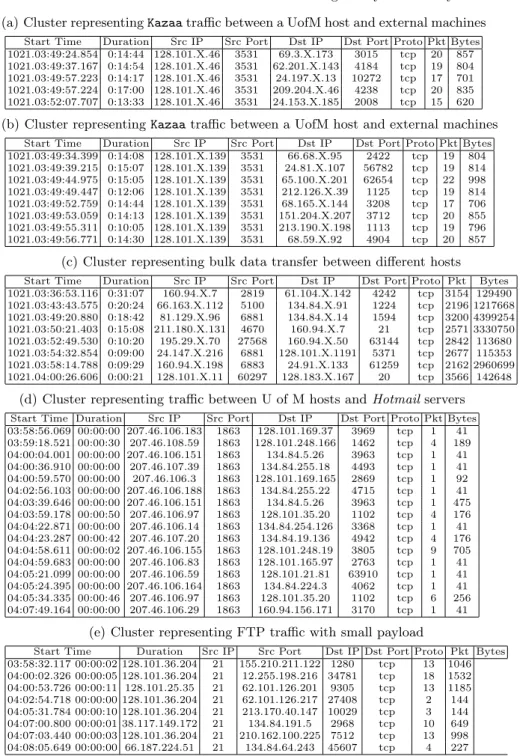
Min-nesota network data. The first two clusters (Tables 6(a) and 6(b)) representKazaa
(a)
Start Time Duration Src IP Src Port Dst IP Dst Port Proto Pkt Bytes 10:00:10.428036 0:00:00 A 4125 B 8200 tcp 5 248 10:00:40.685520 0:00:03 A 4127 B 8200 tcp 5 248 10:00:58.748920 0:00:00 A 4138 B 8200 tcp 5 248 10:01:44.138057 0:00:00 A 4141 B 8200 tcp 5 248 10:01:59.267932 0:00:00 A 4143 B 8200 tcp 5 248 10:02:44.937575 0:00:01 A 4149 B 8200 tcp 5 248 10:04:00.717395 0:00:00 A 4163 B 8200 tcp 5 248 10:04:30.976627 0:00:01 A 4172 B 8200 tcp 5 248 10:04:46.106233 0:00:00 A 4173 B 8200 tcp 5 248 10:05:46.715539 0:00:00 A 4178 B 8200 tcp 5 248 10:06:16.975202 0:00:01 A 4180 B 8200 tcp 5 248 10:06:32.105013 0:00:00 A 4181 B 8200 tcp 5 248 10:07:32.624600 0:00:00 A 4185 B 8200 tcp 5 248 10:08:18.013525 0:00:00 A 4188 B 8200 tcp 5 248 10:08:48.273214 0:00:00 A 4190 B 8200 tcp 5 248 10:09:03.642970 0:00:00 A 4191 B 8200 tcp 5 248 10:09:33.902846 0:00:01 A 4193 B 8200 tcp 5 248 (b)
Start Time Duration Src IP Src Port Dst IP Dst Port Proto Pkt Bytes 10:01:00.181261 0:00:00 A 1176 B 161 udp 1 95 10:01:23.183183 0:00:00 A -1 B -1 icmp 1 84 10:02:54.182861 0:00:00 A 1514 B 161 udp 1 95 10:03:03.196850 0:00:00 A -1 B -1 icmp 1 84 10:04:45.179841 0:00:00 A -1 B -1 icmp 1 84 10:06:27.180037 0:00:00 A -1 B -1 icmp 1 84 10:09:48.420365 0:00:00 A -1 B -1 icmp 1 84 10:11:04.420353 0:00:00 A 3013 B 161 udp 1 95 10:11:30.420766 0:00:00 A -1 B -1 icmp 1 84 10:12:47.421054 0:00:00 A 3329 B 161 udp 1 95 10:13:12.423653 0:00:00 A -1 B -1 icmp 1 84 10:14:53.420635 0:00:00 A -1 B -1 icmp 1 84 10:16:33.420625 0:00:00 A -1 B -1 icmp 1 84 10:18:15.423915 0:00:00 A -1 B -1 icmp 1 84 10:19:57.421333 0:00:00 A -1 B -1 icmp 1 84 10:21:38.421085 0:00:00 A -1 B -1 icmp 1 84 10:21:57.422743 0:00:00 A 1049 B 161 udp 1 168 (c)
Start Time Duration Src IP Src Port Dst IP Dst Port Proto Pkt Bytes 10:10:57.097108 0:00:00 A 3004 B 21 tcp 7 318 10:11:27.113230 0:00:00 A 3007 B 21 tcp 7 318 10:11:37.111176 0:00:00 A 3008 B 21 tcp 7 318 10:11:57.118231 0:00:00 A 3011 B 21 tcp 7 318 10:12:17.125220 0:00:00 A 3013 B 21 tcp 7 318 10:12:37.132428 0:00:00 A 3015 B 21 tcp 7 318 10:13:17.146391 0:00:00 A 3020 B 21 tcp 7 318 10:13:37.153713 0:00:00 A 3022 B 21 tcp 7 318 10:14:47.178228 0:00:00 A 3031 B 21 tcp 7 318 10:15:47.199100 0:00:00 A 3040 B 21 tcp 7 318 10:16:07.206450 0:00:00 A 3042 B 21 tcp 7 318 10:16:47.220403 0:00:00 A 3047 B 21 tcp 7 318 10:17:17.231042 0:00:00 A 3050 B 21 tcp 7 318 10:17:27.234578 0:00:00 A 3051 B 21 tcp 7 318 10:17:37.241179 0:00:00 A 3052 B 21 tcp 7 318 10:17:47.241807 0:00:00 A 3054 B 21 tcp 7 318 10:17:57.247902 0:00:00 A 3055 B 21 tcp 7 318 10:19:07.269827 0:00:00 A 3063 B 21 tcp 7 318 10:19:27.276831 0:00:00 A 3065 B 21 tcp 7 318 10:20:07.291046 0:00:00 A 3072 B 21 tcp 7 318
Table 5. Clusters obtained from network traffic at a US Army Fort, representing
(a) connections toGoToMyPC.com, (b) mis-configured computers subjected to SNMP
Kazaausage is not allowed in the university, this cluster brings forth an anomalous profile for the network analyst to investigate. Cluster in Table 6(c) represents traffic involving bulk data transfers between internal and external hosts; i.e. this cluster covers traffic in which the number of packets and bytes are much larger than the normal values for the involved IPs and ports. Cluster in Table 6(d) represents traffic
between different U of M hosts andHotmailservers (characterized by the port 1863).
Cluster in Table 6(e) representsftptraffic in which the data transferred is low. This
cluster has different machines connecting to different ftp servers all of which are
transferring much lower amount of data than the usual values forftptraffic. A key
observation to be made is that the clustering algorithm automatically determines the dimensions of interest in different clusters. In clusters of Table 6(a),6(b), the protocol, source port and the number of bytes are similar. In cluster of Table 6(c) the only common characteristic is large number of bytes. The common character-istics in cluster of Table 6(d) are the protocol and the source port. In cluster of Table 6(e) the common features are the protocol, source port and the low number of packets transferred.
5 Scan Detection
A precursor to many attacks on networks is often a reconnaissance operation, more commonly referred to as a scan. Identifying what attackers are scanning for can alert a system administrator or security analyst to what services or types of computers are being targeted. Knowing what services are being targeted before an attack allows an administrator to take preventative measures to protect the resources e.g. installing patches, firewalling services from the outside, or removing services on machines which do not need to be running them.
Given its importance, the problem of scan detection has been given a lot of at-tention by a large number of researchers in the network security community. Initial solutions simply counted the number of destination IPs that a source IP made con-nection attempts to on each destination port and declared every source IP a scanner whose count exceeded a threshold [19]. Many enhancements have been proposed re-cently [23, 11, 18, 14, 17, 16], but despite the vast amount of expert knowledge spent on these methods, current, state-of-the-art solutions still suffer from high percent-age of false alarms or low ratio of scan detection. For example, a recently developed scheme by Jung [11] has better performance than many earlier methods, but its performance is dependent on the selection of the thresholds. If a high threshold is selected, TRW will report only very few false alarms, but its coverage will not be satisfactory. Decreasing the threshold will increase the coverage, but only at the cost of introducing false alarms. P2P traffic and backscatter have patterns that are similar to scans, as such traffic results in many unsuccessful connection attempts from the same source to several destinations. Hence such traffic leads to false alarms by many existing scan detection schemes.
MINDS uses a data-mining-based approach to scan detection. Here we present an overview of this scheme and show that an off-the-shelf classifier, Ripper [5], can achieve outstanding performance both in terms of missing only very few scanners and also in terms of very low false alarm rate. Additional details are available in [20, 21].
(a) Cluster representingKazaatraffic between a UofM host and external machines
Start Time Duration Src IP Src Port Dst IP Dst Port Proto Pkt Bytes 1021.03:49:24.854 0:14:44 128.101.X.46 3531 69.3.X.173 3015 tcp 20 857 1021.03:49:37.167 0:14:54 128.101.X.46 3531 62.201.X.143 4184 tcp 19 804 1021.03:49:57.223 0:14:17 128.101.X.46 3531 24.197.X.13 10272 tcp 17 701 1021.03:49:57.224 0:17:00 128.101.X.46 3531 209.204.X.46 4238 tcp 20 835 1021.03:52:07.707 0:13:33 128.101.X.46 3531 24.153.X.185 2008 tcp 15 620
(b) Cluster representingKazaatraffic between a UofM host and external machines
Start Time Duration Src IP Src Port Dst IP Dst Port Proto Pkt Bytes 1021.03:49:34.399 0:14:08 128.101.X.139 3531 66.68.X.95 2422 tcp 19 804 1021.03:49:39.215 0:15:07 128.101.X.139 3531 24.81.X.107 56782 tcp 19 814 1021.03:49:44.975 0:15:05 128.101.X.139 3531 65.100.X.201 62654 tcp 22 998 1021.03:49:49.447 0:12:06 128.101.X.139 3531 212.126.X.39 1125 tcp 19 814 1021.03:49:52.759 0:14:44 128.101.X.139 3531 68.165.X.144 3208 tcp 17 706 1021.03:49:53.059 0:14:13 128.101.X.139 3531 151.204.X.207 3712 tcp 20 855 1021.03:49:55.311 0:10:05 128.101.X.139 3531 213.190.X.198 1113 tcp 19 796 1021.03:49:56.771 0:14:30 128.101.X.139 3531 68.59.X.92 4904 tcp 20 857
(c) Cluster representing bulk data transfer between different hosts
Start Time Duration Src IP Src Port Dst IP Dst Port Proto Pkt Bytes 1021.03:36:53.116 0:31:07 160.94.X.7 2819 61.104.X.142 4242 tcp 3154 129490 1021.03:43:43.575 0:20:24 66.163.X.112 5100 134.84.X.91 1224 tcp 2196 1217668 1021.03:49:20.880 0:18:42 81.129.X.96 6881 134.84.X.14 1594 tcp 3200 4399254 1021.03:50:21.403 0:15:08 211.180.X.131 4670 160.94.X.7 21 tcp 2571 3330750 1021.03:52:49.530 0:10:20 195.29.X.70 27568 160.94.X.50 63144 tcp 2842 113680 1021.03:54:32.854 0:09:00 24.147.X.216 6881 128.101.X.1191 5371 tcp 2677 115353 1021.03:58:14.788 0:09:29 160.94.X.198 6883 24.91.X.133 61259 tcp 2162 2960699 1021.04:00:26.606 0:00:21 128.101.X.11 60297 128.183.X.167 20 tcp 3566 142648
(d) Cluster representing traffic between U of M hosts andHotmailservers
Start Time Duration Src IP Src Port Dst IP Dst Port Proto Pkt Bytes 03:58:56.069 00:00:00 207.46.106.183 1863 128.101.169.37 3969 tcp 1 41 03:59:18.521 00:00:30 207.46.108.59 1863 128.101.248.166 1462 tcp 4 189 04:00:04.001 00:00:00 207.46.106.151 1863 134.84.5.26 3963 tcp 1 41 04:00:36.910 00:00:00 207.46.107.39 1863 134.84.255.18 4493 tcp 1 41 04:00:59.570 00:00:00 207.46.106.3 1863 128.101.169.165 2869 tcp 1 92 04:02:56.103 00:00:00 207.46.106.188 1863 134.84.255.22 4715 tcp 1 41 04:03:39.646 00:00:00 207.46.106.151 1863 134.84.5.26 3963 tcp 1 475 04:03:59.178 00:00:50 207.46.106.97 1863 128.101.35.20 1102 tcp 4 176 04:04:22.871 00:00:00 207.46.106.14 1863 134.84.254.126 3368 tcp 1 41 04:04:23.287 00:00:42 207.46.107.20 1863 134.84.19.136 4942 tcp 4 176 04:04:58.611 00:00:02 207.46.106.155 1863 128.101.248.19 3805 tcp 9 705 04:04:59.683 00:00:00 207.46.106.83 1863 128.101.165.97 2763 tcp 1 41 04:05:21.099 00:00:00 207.46.106.59 1863 128.101.21.81 63910 tcp 1 41 04:05:24.395 00:00:00 207.46.106.164 1863 134.84.224.3 4062 tcp 1 41 04:05:34.335 00:00:46 207.46.106.97 1863 128.101.35.20 1102 tcp 6 256 04:07:49.164 00:00:00 207.46.106.29 1863 160.94.156.171 3170 tcp 1 41
(e) Cluster representing FTP traffic with small payload
Start Time Duration Src IP Src Port Dst IP Dst Port Proto Pkt Bytes 03:58:32.117 00:00:02 128.101.36.204 21 155.210.211.122 1280 tcp 13 1046 04:00:02.326 00:00:05 128.101.36.204 21 12.255.198.216 34781 tcp 18 1532 04:00:53.726 00:00:11 128.101.25.35 21 62.101.126.201 9305 tcp 13 1185 04:02:54.718 00:00:00 128.101.36.204 21 62.101.126.217 27408 tcp 2 144 04:05:31.784 00:00:10 128.101.36.204 21 213.170.40.147 10029 tcp 3 144 04:07:00.800 00:00:01 38.117.149.172 21 134.84.191.5 2968 tcp 10 649 04:07:03.440 00:00:03 128.101.36.204 21 210.162.100.225 7512 tcp 13 998 04:08:05.649 00:00:00 66.187.224.51 21 134.84.64.243 45607 tcp 4 227
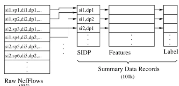
si1,sp1,di1,dp1,... . . . si1,sp4,di2,dp2,... si2,sp3,di2,dp1,... si1,sp2,di2,dp1,... si2,sp5,di3,dp3,... si2,sp6,di3,dp2,... si2,dp1 si1,dp2 si1,dp1 . . . . . . . . .
SIDP Features Label
Raw NefFlows
Summary Data Records .
. .
(5M)
(100k)
Fig. 3.Transformation of raw netflow data in an observation window to the
Sum-mary Data Set. Features are constructed using the set of netflows in the observation window. Labels for use in the training and test sets are constructed by analyzing the data over a long period (usually several days)
Methodology
Currently our solution is a batch-mode implementation that analyzes data in win-dows of 20 minutes. For each 20-minute observation period, we transform the
NetFlow data into asummary data set. Figure 3 depicts this process. With our
focus on incoming scans, each new summary record corresponds to a potential
scanner—that is pair of external source IP and destination port (SIDP). For each SIDP, the summary record contains a set of features constructed from the raw netflows available during the observation window. Observation window size of 20 minutes is somewhat arbitrary. It needs to be large enough to generate features that have reliable values, but short enough so that the construction of summary records does not take too much time or memory.
Given a set of summary data records corresponding to an observation period, scan detection can be viewed as a classification problem [24] in which each SIDP,
whose source IP is external to the network being observed, is labeled as scanner
if it was found scanning ornon-scannerotherwise. This classification problem can
be solved using predictive modeling techniques developed in the data mining and
machine learning community if class labels (scanner/non-scanner) are available for
a set of SIDPs that can be used as a training set.
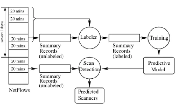
Figure 4 depicts the overall paradigm. Each SIDP in the summary data set for an observation period (typically 20 minutes) is labeled by analyzing the behavior of the source IPs over a period of several days. Once a training set is constructed, a predictive model is built using Ripper. The Ripper generated model can now be used on any summary data set to produce labels of SIDPs.
The success of this method depends on (1) whether we can label the data accu-rately and (2) whether we have derived the right set of features that facilitate the extraction of knowledge. In the following sections, we will elaborate on these points.
Model Predictive Labeler Predicted Scanners NetFlows 20 mins 20 mins 20 mins 20 mins 20 mins 20 mins Summary Records (unlabeled) Summary Records (labeled) Summary Records (unlabeled) Training Detection Scan several days
Fig. 4. Scan Detection using an off-the-shelf classifier, Ripper. Building a
pre-dictive model: 20 minutes ofNetFlowdata is converted into unlabeled Summary
Record format, which is labeled by the Labeler using several days of data. Predictive
model is built on the labeled Summery Records. Scan Detection: 20 minutes of
data is converted into unlabeled Summary Record format. The predictive model is applied to it resulting in a list of predicted scanners.
application is the necessity to integrate the expert knowledge into the method. A part of the knowledge integration is the derivation of the appropriate features. We make use of two types of expert knowledge. The first type of knowledge consists of a list of inactive IPs, a set of blocked ports and a list of P2P hosts in the network being monitored. This knowledge may be available to the security analyst or can be simply constructed by analyzing the network traffic data over a long period (several weeks or months). Since this information does not change rapidly, this analysis can be done relatively infrequently. The second type of knowledge captures the behavior
of<source IP, destination port>(SIDP) pairs, based on the 20-minute observation
window. Some of these features only use the second type of knowledge, and others use both types of knowledge.
Labeling the Data Set: The goal of labeling is to generate a data set that can
be used as training data set for Ripper. Given a set of summarized records cor-responding to 20-minutes of observation with unknown labels (unknown scanning statuses), the goal is to determine the actual labels with very high confidence. The problem of computing the labels is very similar to the problem of scan detection except that we have the flexibility to observe the behavior of an SIDP over a long
period. This makes it possible to declare certain SIDPs asscannerornon-scanner
with great confidence in many cases. For example, if a source IP s ipmakes a few
failed connection attempts on a specific port in a short time window, it may be
hard to declare it a scanner. But if the behavior ofs ipcan be observed over a long
period of time (e.g. few days), it can be labeled asnon-scanner(if it mostly makes
successful connections on this port) orscanner (if most of its connection attempts
are to destinations that never offered service on this port). However, there will sit-uations, in which the above analysis does not offer any clear-cut evidence one way
on the labeling method, the reader is referred to [20].
Evaluation
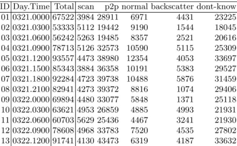
For our experiments, we used real-world network trace data collected at the Uni-versity of Minnesota between the 1st and the 22nd March, 2005. The UniUni-versity of Minnesota network consists of 5 class-B networks with many autonomous sub-networks. Most of the IP space is allocated, but many subnetworks have inactive IPs. We collected information about inactive IPs and P2P hosts over 22 days, and we used flows in 20 minute windows during 03/21/2005 (Mon.) and 03/22/2005 (Tue.) for constructing summary records for the experiments. We took samples of 20-minute duration every 3 hours starting at midnight on March 21. A model was built for each of the 13 periods and tested on the remaining 12 periods. This allowed us to reduce possible dependence on a certain time of the day, and performed our experiments on each sample.
Table 7 describes the traffic in terms of number of<source IP, destination port>
(SIDP) combinations pertaining to scanning-, P2P-, normal- and backscatter traffic.
Table 7.The distribution of (source IP, destination ports) (SIDPs) over the various
traffic types for each traffic sample produced by our labeling method
ID Day.Time Total scan p2p normal backscatter dont-know
01 0321.0000 67522 3984 28911 6971 4431 23225 02 0321.0300 53333 5112 19442 9190 1544 18045 03 0321.0600 56242 5263 19485 8357 2521 20616 04 0321.0900 78713 5126 32573 10590 5115 25309 05 0321.1200 93557 4473 38980 12354 4053 33697 06 0321.1500 85343 3884 36358 10191 5383 29527 07 0321.1800 92284 4723 39738 10488 5876 31459 08 0321.2100 82941 4273 39372 8816 1074 29406 09 0322.0000 69894 4480 33077 5848 1371 25118 10 0322.0300 63621 4953 26859 4885 4993 21931 11 0322.0600 60703 5629 25436 4467 3241 21930 12 0322.0900 78608 4968 33783 7520 4535 27802 13 0322.1200 91741 4130 43473 6319 4187 33632
In our experimental evaluation, we provide comparison to TRW [11], as it is one of the state-of-the-art schemes. With the purpose of applying TRW for scanning worm containment, Weaver et al. [25] proposed a number of simplifications so that TRW can be implemented in hardware. One of the simplifications they applied— without significant loss of quality—is to perform the sequential hypothesis testing in logarithmic space. TRW then can be modeled as counting: a counter is assigned to each source IP and this counter is incremented upon a failed connection attempt and decremented upon a successful connection establishment.
Our implementation of TRW used in this paper for comparative evaluation draws from the above ideas. If the count exceeds a certain positive threshold, we declare the source to be scanner, and if the counter falls below a negative threshold, we declare the source to be normal.
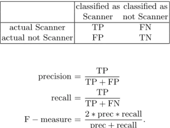
The performance of a classifier is measured in terms of precision, recall and F-measure. For a contingency table of
classified as classified as
Scanner not Scanner
actual Scanner TP FN
actual not Scanner FP TN
precision = TP
TP + FP
recall = TP
TP + FN
F−measure = 2∗prec∗recall
prec + recall .
Less formally, precision measures the percentage of scanning (source IP, des-tination port)-pairs (SIDPs) among the SIDPs that got declared scanners; recall measures the percentage of the actual scanners that were discovered; F-measure balances between precision and recall.
To obtain a high-level view of the performance of our scheme, we built a model on the 0321.0000 data set (ID 1) and tested it on the remaining 12 data sets. Figure 5 depicts the performance of our proposed scheme and that of TRW on the same
data sets4.
One can see that not only does our proposed scheme outperform TRW by a wide margin, it is also more stable: the performance varies less from data set to data set (the boxes in Figure 5 appear much smaller).
Figure 6 shows the actual values of precision, recall and F-measure for the dif-ferent data sets. The performance in terms of F-measure is consistently above 90% with very high precision, which is important, because high false alarm rates can rapidly deteriorate the usability of a system. The only jitter occurs on data set # 7 and it was caused by a single source IP that scanned a single destination host on 614(!) different destination ports meanwhile touching only 4 blocked ports. This source IP got misclassified as P2P, since touching many destination ports (on a number of IPs) is characteristic of P2P. This single misclassification introduced 614 false negatives (recall that we are classifying SIDPs not source IPs). The reason for the misclassification is that there were no vertical scanners in the training set — the highest number of destination ports scanned by a single source IP was 8, and this source IP touched over 47 destination IPs making it primarily a horizontal scanner.
4 The authors of TRW recommend a threshold of 4. In our experiments, we found,
that TRW can achieve better performance (in terms of F-measure) when we set the threshold to 2, this is the threshold that was used in Figure 5, too.
Prec Rec F−m Prec Rec F−m 0 0.2 0.4 0.6 0.8 1 Ripper TRW Performance Comparison
Fig. 5.Performance comparison between the proposed scheme and TRW. From left
to right, the six box plots correspond to the precision, recall and F-measure of our proposed scheme and the precision, recall and F-measure of TRW. Each box plot has three lines corresponding (from top downwards) to the upper quartile, median and lower quartile of the performance values obtained over the 13 data sets. The whiskers depict the best and worst performance.
3 5 7 9 11 13 0 0.2 0.4 0.6 0.8 1 Test Set ID Performance of Ripper Precision Recall F−measure
Fig. 6. The performance of the proposed scheme on the 13 data sets in terms
of precision (topmost line), F-measure (middle line) and recall (bottom line). The model was built on data set ID 1.
6 Conclusion
MINDSis a suite of data mining algorithms which can be used as a tool by network analysts to defend the network against attacks and emerging cyber threats. The
various components ofMINDS such as the scan detector, anomaly detector and the
profiling module detect different types of attacks and intrusions on a computer network. The scan detector aims at detecting scans which are the percusors to any network attack. The anomaly detection algorithm is very effective in detecting behavioral anomalies in the network traffic which typically translate to malicious
activities such asdostraffic, worms, policy violations and inside abuse. The profiling
module helps a network analyst to understand the characteristics of the network traffic and detect any deviations from the normal profile. Our analysis shows that
the intrusions detected byMINDSare complementary to those of traditional signature based systems, such as SNORT, which implies that they both can be combined
to increase overall attack coverage. MINDS has shown great operational success in
detecting network intrusions in two live deployments at the University of Minnesota and as a part of the Interrogator [15] architecture at the US Army Research Labs Center for Intrusion Monitoring and Protection (ARL-CIMP).
7 Acknowledgements
This work is supported by ARDA grant AR/F30602-03-C-0243, NSF grants IIS-0308264 and ACI-0325949, and the US Army High Performance Computing Re-search Center under contract DAAD19-01-2-0014. The reRe-search reported in this article was performed in collaboration with Paul Dokas, Yongdae Kim, Aleksan-dar Lazarevic, Haiyang Liu, Mark Shaneck, Jaideep Srivastava, Michael Steinbach, Pang-Ning Tan, and Zhi-li Zhang. Access to computing facilities was provided by the AHPCRC and the Minnesota Supercomputing Institute.
References
1. Rakesh Agrawal, Tomasz Imieliski, and Arun Swami. Mining association rules
between sets of items in large databases. InProceedings of the 1993 ACM
SIG-MOD international conference on Management of data, pages 207–216. ACM Press, 1993.
2. Daniel Barbara and Sushil Jajodia, editors. Applications of Data Mining in
Computer Security. Kluwer Academic Publishers, Norwell, MA, USA, 2002. 3. Markus M. Breunig, Hans-Peter Kriegel, Raymond T. Ng, and J Sander. Lof:
identifying density-based local outliers. InProceedings of the 2000 ACM
SIG-MOD international conference on Management of data, pages 93–104. ACM Press, 2000.
4. Varun Chandola and Vipin Kumar. Summarization – compressing data into an
informative representation. In Fifth IEEE International Conference on Data
Mining, pages 98–105, Houston, TX, November 2005.
5. William W. Cohen. Fast effective rule induction. InInternational Conference
on Machine Learning (ICML), 1995.
6. Dorothy E. Denning. An intrusion-detection model. IEEE Trans. Softw. Eng.,
13(2):222–232, 1987.
7. Eric Eilertson, Levent Ert¨oz, Vipin Kumar, and Kerry Long. Minds – a new
approach to the information security process. In 24thArmy Science Conference.
US Army, 2004.
8. Levent Ert¨oz, Eric Eilertson, Aleksander Lazarevic, Pang-Ning Tan, Vipin Ku-mar, Jaideep Srivastava, and Paul Dokas. MINDS - Minnesota Intrusion
Detec-tion System. In Data Mining - Next Generation Challenges and Future
Direc-tions. MIT Press, 2004.
9. Levent Ertoz, Michael Steinbach, and Vipin Kumar. Finding clusters of different
sizes, shapes, and densities in noisy, high dimensional data. In Proceedings of
10. Anil K. Jain and Richard C. Dubes. Algorithms for Clustering Data. Prentice-Hall, Inc., 1988.
11. Jaeyeon Jung, Vern Paxson, Arthur W. Berger, and Hari Balakrishnan. Fast
portscan detection using sequential hypothesis testing. InIEEE Symposium on
Security and Privacy, 2004.
12. Vipin Kumar, Jaideep Srivastava, and Aleksander Lazarevic, editors.Managing
Cyber Threats–Issues, Approaches and Challenges. Springer Verlag, May 2005. 13. Aleksandar Lazarevic, Levent Ert¨oz, Vipin Kumar, Aysel Ozgur, and Jaideep Srivastava. A comparative study of anomaly detection schemes in network
in-trusion detection. InSIAM Conference on Data Mining (SDM), 2003.
14. C. Lickie and R. Kotagiri. A probabilistic approach to detecting network scans. InEighth IEEE Network Operations and Management, 2002.
15. Kerry Long. Catching the cyber-spy, arl’s interrogator. In 24th Army Science
Conference. US Army, 2004.
16. V. Paxon. Bro: a system for detecting network intruders in real-time. InEighth
IEEE Network Operators and Management Symposium (NOMS), 2002. 17. Phillip A. Porras and Alfonso Valdes. Live traffic analysis of tcp/ip gateways.
InNDSS, 1998.
18. Seth Robertson, Eric V. Siegel, Matt Miller, and Salvatore J. Stolfo. Surveillance
detection in high bandwidth environments. InDARPA DISCEX III Conference,
2003.
19. Martin Roesch. Snort: Lightweight intrusion detection for networks. InLISA,
pages 229–238, 1999.
20. Gyorgy Simon, Hui Xiong, Eric Eilertson, and Vipin Kumar. Scan detection: A data mining approach. Technical Report AHPCRC 038, University of Minnesota – Twin Cities, 2005.
21. Gyorgy Simon, Hui Xiong, Eric Eilertson, and Vipin Kumar. Scan detection:
A data mining approach. InProceedings of SIAM Conference on Data Mining
(SDM), 2006.
22. Anoop Singhal and Sushil Jajodia. Data mining for intrusion detection. InData
Mining and Knowledge Discovery Handbook, pages 1225–1237. Springer, 2005. 23. Stuart Staniford, James A. Hoagland, and Joseph M. McAlerney. Practical
automated detection of stealthy portscans. Journal of Computer Security,
10(1/2):105–136, 2002.
24. Pang-Ning Tan, Michael Steinbach, and Vipin Kumar. Introduction to Data
Mining. Addison-Wesley, May 2005.
25. Nicholas Weaver, Stuart Staniford, and Vern Paxson. Very fast containment of