Optimal Fiscal Policy in a Monetary Union

(1)

CENTER FOR FISCAL POLICY

CFI

Optimal Fiscal Policy in a Monetary Union

by

Luisa Lambertini

January 2007

Center for Fiscal Policy Working Paper Series

(2)

Optimal Fiscal Policy in a Monetary Union

∗

by

Luisa Lambertini

EPFL and Claremont McKenna College

January 2007

Abstract

We study optimal fiscal policy in a monetary union where monetary policy is decided by an independent central bank. We consider a two-country model with trade in goods and assets, augmented with sticky prices, labor income taxes and stochastic government consumption. It is optimal to finance a shock in part by running deficits and in part by raising the labor income tax, even though the latter is distortionary. The optimal speed of adjustment of budget deficits is much higher than the benchmark adjustment of 0.5 percent of GDP per year required by the recent revision of the Stability and Growth Pact (SGP). Optimal fiscal policy does not depend on the initial level of public debt. Ramsey monetary policy allows for less aggressive and more expansionary response of fiscal policy than the monetary policy implied by an interest rates rule.

Address of author:

Luisa Lambertini, Department of Economics, Claremont McKenna College, 500 E. 9th Street, Claremont, CA 91711, USA. E-mail: luisa.lambertini@cmc.edu

∗_{This paper has been originally written for presentation at the conference: “Five Years of the Euro:}

Successes and New Challenges,” Federal Reserve Bank of Dallas, May 14-16, 2004. I have benefited from the comments of Nicola Giammarioli, Leo von Thadden and participants of the conference on “New Perspective on Fiscal Sustainability,” the Konstanz Seminar on Monetary Policy 2006 and of seminars at the ECB, Boston College, Boston University, Claremont McKenna College and GREQAM. The usual disclaimer applies.

(3)

1 Introduction

The creation of the Economic and Monetary Union (EMU) in Europe has put much emphasis on the design of monetary and fiscal institutions and on encouraging fiscal discipline among the member states. This has materialized in the Maastricht Treaty and its subsequent pacts that forbid the European Central Bank (ECB) from purchasing member states’ debts or bailing them out, even in the event of a fiscal crisis, and require it to pursue price stability. The Stability and Growth Pact (SGP), in its original formulation, establishes that EMU members should not run deficits in excess of 3 percent of GDP, except in deep recessions, and that fiscal policy should aim to bring the debt to GDP ratio to about 0.6 and balance the budget over the business cycle after that. The rationale behind fiscal limits in the EMU, according to its proponents, was the fear of excessive deficits and pressure on the ECB with untested reputation to monetize such deficits.

Repeated violations of the deficit limits stipulated by the SGP and difficulties in imple-menting the established procedures for countries in violation of such limits led to a revision of the SGP in 2005 aimed to increase its flexibility and to improve the implementability of the pact. The increase in flexibility came with a broader definition of “severe economic downturn” to include prolonged period of low growth and with the introduction of relevant factors, such as significant economic reforms, in the judgement used for triggering an ex-cessive deficit procedure. The improved implementability took the form of country-specific medium-term objectives in cyclically adjusted terms and the introduction of a benchmark adjustment of 0.5 percent of GDP per year for countries with deficits higher than their medium-term objectives.

By now, the SGP regulates several dimensions of fiscal policy, from the size of the deficit to the speed of adjustment, the medium-term budget balances and the long-run public debt level. An important component of an analysis of fiscal policy and fiscal limits is the fully optimal fiscal policy. This is the benchmark against which to compare actual policies and fiscal limits should drive actual policies close to such benchmark.

This paper characterizes optimal fiscal policy in a monetary union. This is the policy that can be achieved by commitment by solving the Ramsey problem. We consider a two-country model that trade in goods and assets augmented with sticky prices; both countries belong to a monetary union and the common monetary policy is decided by an independent central bank. Government spending as well as technology are stochastic and each government decides fiscal policy in its own country by setting the labor income tax and by deciding how much public debt to issue.

We find that it is optimal to finance a shock, for example an unanticipated increase in government spending, in part by running a deficit and in part by raising income taxes. There are two reasons why taxes are raised even if they are distortionary. First, the price level cannot be raised instantaneously to inflate public debt away because monetary policy follows an interest rate rule that responds to inflation. Second, even optimal monetary policy would not inflate public debt away completely because this would be costly in our setup with sticky prices. As a result, optimal fiscal policy entails an increase in the labor income tax

(4)

and budget deficits that spread the tax increase over time.

The optimal unconditional net financial position of the fiscal authority is a credit large enough to finance, with its interest income, steady-state government spending and labor sub-sidies aimed at eliminating the distortion stemming from monopolistic competition. Condi-tional on a given initial level of public debt, the optimal level of public debt is a random walk in our model. In flexible price models, like in Chari et al. (1991), optimal monetary policy inflates any initial level of government debt away in the first period. This is not the case in our setup because the central bank follows an interest rate rule. Even if monetary policy is optimal, it does not inflate the initial debt away in our model because the large increase in the initial price level would persist over time in our setup, distorting relative prices and consumption choices.

Optimal fiscal policy is does not depend on the initial level of public debt. Ramsey fiscal policy commands the same response of public debt and taxes independently of the initial debt level.1

Monetary and fiscal policy interact in important ways. By changing the nominal interest rate, the central bank affects the borrowing cost and therefore the extent to which optimal fiscal policy relies on deficit versus tax financing. Interest rate rules that imply a more aggressive increase of the nominal interest rate in response to a government spending shock are associated with less persistent deficits. In response to a government spending shock, the Ramsey planner reduces the nominal interest rate and the tax rate. This results in a strong response of hours that raises output and makes the fiscal shock expansionary in the short run.

Optimal fiscal policy in one country of the monetary union responds to shocks in other countries of the union. There are a number of reasons for this result. First, we characterize cooperative optimal fiscal policy in the monetary union. Second, countries trade in goods and assets. Third, monetary policy responds to union-wide variables so that a shock in one country triggers an interest rate response by the common central bank.

2 Existing Literature

The existing literature studies the determination of optimal monetary and fiscal policy when the government problem is to finance an exogenous stream of public consumption by levying taxes and issuing debt and money so as to maximize welfare. Optimal monetary and fiscal policies depend on the environment in which they operate. When prices are flexible, com-petition is perfect and government debt is state contingent, as in Lucas and Stokey (1983), government debt and tax rates inherit the stochastic process of the exogenous shocks. When government debt is nominally non-state-contingent, as in Chari et al. (1991), the government finds it optimal to use inflation as a lump-sum tax on financial wealth; as a result inflation is highly volatile while the tax rate remains stable over the business cycle. This result is robust to the introduction of monopolistic competition in the goods market, as shown by

(5)

Schmitt-Grohe and Uribe (2004d).

Some papers have focused on studying optimal monetary policy in an environment with nominal rigidities and monopolistic competition. Part of this literature assumes that the government has access to lump-sum taxes to finance its consumption and that it can im-plement a production subsidy that eliminates the inefficiency stemming from monopolistic competition.2 _{As a result, the optimal inflation rate is stable and close to zero. Intuitively,}

lump-sum taxes are used to finance government spending without creating distortions and prices can remain stable to minimize the costs of inflation in an environment with price rigidities. Schmitt-Grohe and Uribe (2004a) depart from this literature by studying optimal monetary and fiscal policy in a model where the government can resort only to distortionary income taxation and issue only nominal non-state-contingent bonds. Schmitt-Grohe and Uribe find that optimal inflation volatility is almost zero even for low degrees of price sticki-ness. Correia et al. (2003) enrich the set of fiscal instruments and find that the set of frontier implementable allocations does not depend on the degree of price stickiness.

We find that public debt and tax rates follow a random walk behavior in our model. This result is consistent with the findings of Aiyagari et al. (2002) and Schmitt-Grohe and Uribe (2004a), which assume like us that government debt is non-state contingent. Our work is different as it extends the analysis to an open economy with a monetary union.

A number of papers focus on the interaction of monetary and fiscal policies. Dixit and Lambertini (2003a) and Lambertini (2004) study the strategic interaction between a conservative and independent central bank and a benevolent fiscal authority that maximizes social welfare in models where purpose of fiscal policy is to stabilize prices and output. In such setting, equilibrium outcomes are suboptimal when policies are discretionary and even when monetary policy is committed but fiscal policy is discretionary. The optimal design of institutions assigns non-conflicting goals to the authorities and, if policies are discretionary, the price goal should be appropriately conservative. Dixit and Lambertini (2001, 2003b) extend this analysis to a monetary union and find that the spillover of one country’s fiscal policy on others exacerbates the suboptimality of the equilibrium. Sibert (1992), Levine and Brociner (1994) and Beetsma and Bovenberg (1998) consider monetary-fiscal interactions in a monetary union where the purpose of fiscal policy is to provide public goods. Chari and Kehoe (2004) conclude that fiscal limits are desirable in a monetary union when the central bank cannot commit in advance. We depart from this literature in two ways. First, we assume that government spending is exogenous and stochastic and that the problem faced by the fiscal authority is how to finance such spending stream in the least disruptive way. Second, we assume that the fiscal authority can commit to its policies and the central bank can commit to follow an interest rate rule. Third, the central bank and the fiscal authority have non-conflicting goals.

There is a large literature on the SGP, too large to be reviewed here. Eichengreen and Wyplosz (1998) suggest that the SGP is likely to affect the fiscal behavior of EMU members

2_{See Erceg et al. (2000), Gal´ı and Monacelli (2000), Khan et a. (2000), Rotemberg and Woodford (1999)}

(6)

and to partly hamper automatic stabilizers,3 _{thereby wondering if the SGP will only be a}

“minor nuisance”. Beetsma and Debrun (2004, 2005) argue that fiscal limits ´a la SGP help reduce the deficit bias of electorally-motivated governments but also reduce spending on “high-quality” outlays such as public investment and other outlays typically associated with economic reforms. Wyplosz (2005, 2006) argue that the SGP is flawed, even though it has influenced policymakers in the sense that fiscal policy would have likely been less disciplined than they have been. Nevertheless, fiscal policy should follow the lead from monetary policy and move from discretion to rules and then to institutions. This logical sequence has been put into practice for monetary policy and it has worked remarkably well. We contribute to this literature by providing a formal assessment of how often the SGP would bind if fiscal policy were optimal.

3 The Model

The model assumes two countries, country 1 and 2, that belong to a monetary union and share a common currency. Each country has a separate government that run fiscal policy while monetary policy is decided by a common and independent central bank.

The representative household in country 1 has preferences defined over per capita con-sumption C1,t and per capita hours workedN1,t as described by the utility function

Et

∞

X

s=t

βs−tU(C1,s−b1C1,s−1, N1,s) (1)

where 0< β <1 is a discount factor andEt denotes the mathematical expectations operator

conditional on information available at the beginning of period t. Hours worked is given by

N1,t ≡

Z _n

0 N1,t(i)di

where N1,t(i) is the quantity of labor of type i supplied by the representative individual to

domestic firms. It is assumed that each differentiated good uses a specialized labor input in its production and the individual supplies labor input to all domestic firms. Preferences display internal habit formation measured by the parameter b1 ∈[0,1).

There is a continuum of differentiated goods distributed over the interval [0,1]; a fraction

n of these goods is produced in country 1 while the fraction 1−n is produced in country 2.

C1,t is the real consumption index

C1,t = ·Z ₁ 0 C1,t(i) θ−1 θ di ¸ θ θ−1 , (2)

where C1,t(i) is consumption of good i at time t and θ > 1 is the constant elasticity of

substitution among the individual goods. The representative household consumes all goods

3_{Gal´ı and Perotti (2003), however, find no empirical evidence that the SGP has impaired fiscal}

(7)

produced in the world economy. The price indexPt corresponding to the consumption index C1,t is Pt= ·Z ₁ 0 Pt(i) 1−θ_di ¸ 1 1−θ , (3)

which is the minimum cost of a unit of the aggregate consumption good defined by (2), given individual good prices Pt(i).

The representative household in country 2 has symmetric preferences to those in (1) and (2). All households in country 1 begin with the same amount of financial assets and own the same share of domestic firms; ownership of foreign firms is not allowed. The budget constraint in real terms for the representative agent in country 1 is

bp₁_,t 1 +it +C1,t = bp₁_,t₋₁ πt +w1,t(1−τ1,t)N1,t+ Z _n 0 Π1,t n (i)di, (4) where bp₁_,t ≡ B p 1,t Pt , w1,t ≡ W1,t Pt .

Here bp₁_,t is the purchase of a riskless, non-contingent nominal bond in real terms. This bond is the only asset available for borrowing or lending between the two countries and 1 +it is the gross nominal interest rate. w1,t is the real wage in period t; in the absence of

firm-specific technological shocks, all labor types receive the same wage because they have the same marginal productivity. Π1,t(i) are real profits of firm producing good i in country

1. τ1,t is a distortionary income tax levied by the government of country 1 at time t. The

household is subject to the transversality condition lim T→∞qt,T " bp₁_,T₊₁ 1 +iT+1 # = 0 (5)

on financial wealth, where qt,T is the stochastic discount factor. The household maximizes

utility (1) subject to the budget constraint (4). The first-order conditions that describe the agent’s behavior are:

C1,t(i) = Ã Pt(i) Pt !₋_θ C1,t, (6) UC(C1,t−b1C1,t−1)−b1βEtUc(C1,t+1−b1C1,t, N1,t+1) = λ1,t, (7) λ1,t 1 +it =βEt λ1,t+1 πt+1 , (8) −UN(C1,t−b1C1,t−1, N1,t) = λ1,tw1,t(1−τ1,t), (9)

where UC, UN are the marginal utility with respect to consumption and labor, respectively

and λ1,t is the lagrangean multiplier at time t on the agent’s budget constraint. (6) shows

that the agent’s consumption of each differentiated goods is negatively related to its relative price. λ1,t equals the marginal utility of consumption, as stated by (7). (8) is the standard

(8)

Goods are produced by firms that make use only of labor:

Y1,t(i) =A1,tN1,t(i), (10)

where A1,t is an exogenous stochastic technological factor common to all firms in country 1.

Country 2 has a similar production function. Firms maximize the present discounted value of profits. Firm i in country 1 maximizes

Et

∞

X

s=t

qt,sPsΠ1,s(i). (11)

Real profits at time t are sale revenues minus the cost of producing the goods, which is the wage bill:

Π1,t(i) =

Pt(i)

Pt

Y1,t(i)−w1,tN1,t(i). (12)

The firm takes the real wage as given. The demand faced by i−th producer is

Y1,t(i)d = " Pt(i) Pt #₋_θ (Ct+Gt) (13)

where Ct ≡ nC1,t + (1 −n)C2,t is monetary union-wide private consumption and Gt ≡

nG1,t+ (1−n)G2,t is monetary union-wide public consumption.

Prices are sticky. Every period, a fraction φ ∈ [0,1) of randomly chosen firms does not change price and meets demand at the posted price; the remaining fraction 1−φ of firms sets the price optimally. At time t, firms that have the opportunity of changing the price maximize Et ∞ X s=t φs−t_q t,sPs " Pt(i) Ps Ys(i)−w1,s Ys(i) As # +mc1,s  _A_s_N₁_,s₍_i₎₋ Ã Pt(i) Ps !₋_θ Ys  _, ₍₁₄₎

where mc1,t is the Lagrangean multiplier associated with the constraint that production

meets demand. In each period firms choose how much labor to hire and the first-order condition gives:

mc1,t = w1,t

A1,t

. (15)

The associated first-order condition with respect to Pt(i) is

θEt ∞ X s=t φs−t_q t,sYsmc1,s Ã Pt(i) Ps !₋_θ₋₁ = (θ−1)Et ∞ X s=t φs−t_q t,sYs Ã Pt(i) Ps !₋_θ , (16) where Yt =Ct+Gt is aggregate demand, which the firm takes as given. The optimal price

depends on current and expected future marginal costs and demand conditions. Here we limit our attention to a symmetric equilibrium where all firms that can change their prices

(9)

in a country choose the same price. Let ˜p1,t ≡ P˜1,t/Pt, where ˜Pt is the optimal price level

chosen at t by firms in country 1. The dynamics of prices is

1 =φπ_tθ−1+ (1−φ)hnp˜1₁−_,tθ+ (1−n)˜p1₂−_,tθi, (17) where πt≡Pt/Pt−1 is the inflation rate in period t.

Because the model does not assume production subsidies to ensure that long-run output levels are at their competitive levels, we wish to retain the non-linearity of (16) and use second-order linear approximations to the equilibrium conditions for correct welfare evalua-tion. To do that, I follow Schmitt-Grohe and Uribe (2004c) and rewrite (16) as

v1,t

θ

θ−1 =vv1,t, (18)

where the two auxiliary variables v1,t and vv1,t are defined as follows:

v1,t ≡Et ∞ X s=t φs−tqt,sYs w1,s A1,s Ã Pt(i) Ps !₋_θ₋₁ = ˜p−₁_,tθ−1Ytmc1,t+φβEt λ1,t+1 λ1,t π_tθ₊₁ Ã ˜ p1,t ˜ p1,t+1 !₋_θ₋₁ v1,t+1, (19) vv1,t ≡Et ∞ X s=t φs−tqt,sYs Ã Pt(i) Ps !₋_θ = ˜p−₁_,tθYt+φβEt λ1,t+1 λ1,t πθ_t₊₁−1 Ã ˜ p1,t ˜ p1,t+1 !₋_θ vv1,t+1. (20)

A common central bank decides monetary policy for the union and each country’s govern-ment decides fiscal policy for its own country. The central bank is instrugovern-ment-independent in the sense that it chooses monetary policy freely and it does not share the government budget constraints. The central bank follows the interest rate rule

it= ¯i+φy µ Yt−Y Y ¶ +φπ µ πt−π π ¶ +φi(it−1−¯i), (21)

where ¯i is the steady-state value of the nominal interest rate. (21) describes an interest rate rule whereby the central bank sets the nominal rate as a function of the deviations of monetary union-wide output and inflation from their steady state values. It is typically assumed that the coefficient on inflationφπ is greater than one, which implies that the central

bank raises the nominal interest rate in response to an increase in inflation.

The fiscal authority in each country decides how to finance an exogenous and stochastic stream of public consumption. Government spending in country 1, G1,t, is stochastic and

takes the form

G1,t = ·Z ₁ 0 G1,t(i) θ−1 θ di ¸ θ θ−1 , (22)

and similarly for country 2. Cost minimization implies that the government demand for good i has the same form as (6), the agent’s demand for good i. The budget constraint for the government in real terms is

bg₁_,t 1 +it = b g 1,t−1 πt +G1,t−w1,tN1,tτ1,t, (23)

(10)

where bg₁_,t ≡B₁g_,t/Pt.

Let h1,t ≡

R

0,n(Pt(i)/Pt)1−θdi, x1,t ≡

R

0,n(Pt(i)/Pt)−θdi. After some simplifications, these

variables can be written as

h1,t ≡ Z _n 0 Ã Pt(i) Pt !₁₋_θ di=n(1−φ)˜p1−θ 1,t +φπtθ−1h1,t−1, (24) x1,t ≡ Z _n 0 Ã Pt(i) Pt !₋_θ di=n(1−φ)˜p−θ 1,t +φπtθx1,t−1. (25)

In equilibrium, firms meet demand. Integration over all firms in country 1 delivers

nA1,tN1,t = Z _n 0 Ã Pt(i) Pt !₋_θ diYt=x1,tYt (26)

and similar equations hold for country 2. Real aggregate profits in country 1 are

Z _n 0 Πi,tdi= Z _n 0 Ã Pt(i) Pt !₁₋_θ di Yt−w1,tN1,t =h1,tYt−w1,tN1,t. (27)

Equilibrium in the goods market implies

nA1,tN1,t x1,t

+ (1−n)A2,tN2,t

x2,t

=Yt=Ct+Gt, (28)

which implies clearing in the asset market:

n(bg₁_,t−bp₁_,t) + (1−n)(bg₂_,t−bp₂_,t) = 0, ∀t. (29)

4 The Ramsey Problem

Consider now a benevolent planner that decides how to finance an exogenously given stream of public spending in the monetary union so as to maximize utility as given by a weighted average of the two countries’ utilities. Suppose the benevolent planner can commit ex-ante to a sequence of policies. Let n1 = n, n2 = 1− n1. The lagrangean for the benevolent

planner’s problem, which is known as the Ramsey problem, is given in (A.1) in appendix A. The benevolent planner chooses the sequence of tax rates {τs} associated with the

competitive equilibrium that yields the highest level of joint utility in the union. The Ramsey policy functions associated to problem (A.1) form a dynamic system that cannot be solved analytically. As suggested earlier, steady-state output is inefficiently low in this model, thereby violating the set of assumptions that allow welfare to be approximated accurately from a first-order approximation to the equilibrium conditions. For this reason, we compute second-order approximations to the policy functions using the computer code of Schmitt-Grohe and Uribe (2004b).

(11)

5 Calibration

The time unit is a quarter and the period utility function is:

U(C1,t−b1C1,t−1, N1,t) = log(C1,t−b1C1,t−1)−dlog(1−N1,t).

d is equal to 2, which implies that the representative agent works one third of her total time in the steady state. The internal habit persistence stock is assumed to be 55% of past consumption, which is in line with the estimates in Smets and Wouters (2002). The discount factor β is 0.99, which is consistent with a steady-state real rate of return of 4.1 percent a year. Sbordone (2002) and Clarida et al. (1999) suggest that the parameter φ summarizing the degree of price staggering is equal to 2/3 implying that firms on average change prices every three quarters; Bils and Klenow (2004) suggest instead a 4.3 months average lifespan of prices. We follow Bils and Klenow and set the parameter φ equal to 1/3, which implies an average life span of prices of 4.5 months. The steady-state gross inflation rate is one. The mark-up parameter θ is set equal to 11, so that steady-state mark-up is 10 percent, as consistent with the work of Basu and Fernald (1997) and as used in other works that assume price staggering (see for example Gal´ı (2003)). For our benchmark specification, we assume that the interest rate rule responds to inflation and to the lagged nominal interest rate by setting φπ = 1.5 and φi = 0.9. Later on we consider alternative parameter values

along the lines of Smets and Wouters (2002) and Taylor (1993). The size of country 1 is set equal to 0.3, which is consistent with the size of Germany relative to the euro area. Steady-state government consumption is assumed to be 20 percent of GDP in both countries, which is consistent with data from post-war Germany and most members of the EMU. The benchmark simulation features a government debt-to-GDP ratio of 0.6 both in country 1 and 2; private bond holding are assumed to be 0.6 of GDP in country 1 and 2. The steady-state labor income tax rate that balances the government budget is 24% in country 1 and 20% in country 2. Table 1 summarizes the values assigned to the structural parameters of the model.

Government spending and technology are assumed to follow the stochastic processes lnGi,t = (1−ρg) lnGi+ρglnGi,t−1+²gi,t, i= 1,2, (30)

lnAi,t = (1−ρa) lnAi+ρalnAi,t−1+²ai,t, i= 1,2. (31)

The persistence parameters and the standard deviation of the shocks are estimated using data for Germany; their values are given in Table 1.

6 Ramsey Dynamics

With sticky prices and nominally non-state-contingent assets, the Ramsey problem contains a sequence of intertemporal constraints, one for each date and state. This makes it impossible to find an exact numerical solution to the Ramsey problem. This section presents the results of our second-order approximation to the Ramsey’s problem.4 _{Incidentally, a first-order}

(12)

Parameter Value Description

β 0.99 Subjective discount factor

d 2 Calibrated to match N = 0.3

b 0.55 Internal habit

θ 11 Calibrated to match 1.1 gross value-added markup

φ 1/3 Degree of price stickiness

φy 0 Coefficient on output

φπ 1.5 Coefficient on inflation

φi 0.9 Interest-rate smoothing

g/Y 0.2 Government consumption to GDP ratio

bg_/Y _0.6 _{Government debt to GDP ratio}

bp_/Y _0.6 _{Private bond holding as % of GDP}

n1 0.3 Country size

ρg 0.88 Serial correlation of lngt

σg 0.015 Standard deviation of innovation to lngt

ρa 0.9 Serial correlation of lnat

σa 0.02 Standard deviation of innovation to lnat

Table 1: Structural parameters

approximation to the Ramsey equilibrium conditions generates dynamics that are very close to the dynamics associated with a second-order approximation in a closed economy with characteristics similar to those of our model.5

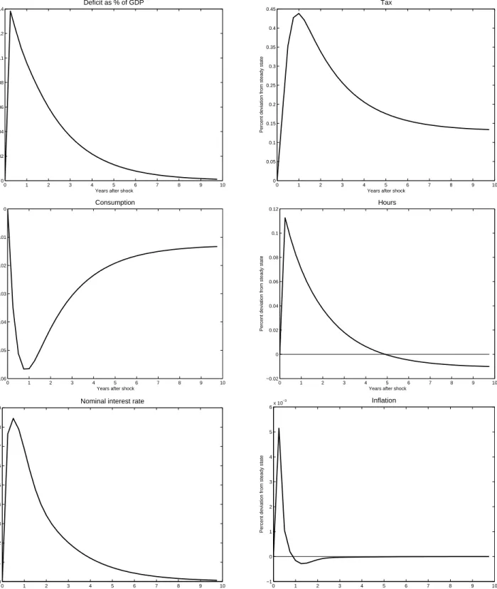
Figure 1 shows the impulse response of some variables in country 1 to a one percentage point increase in government purchases. It is optimal to finance an increase in government spending in part by raising labor income taxes and in part by running budget deficits. Issuing public debt enables the Ramsey planner to keep a smooth tax profile that spreads the distortion over time and to soften the response of private consumption.

Taxes and real public debt display unit-root behavior, as deficits are not followed by surpluses. In response to a one percentage point increase in government spending, real public debt increases by 2 percentage points in the long run. As a consequences of higher debt, the tax rate increases, hours fall and consumption falls at the new steady state.

In a monetary economy with flexible prices, a Ramsey planner that decides monetary and fiscal policy would set the price level equal to ∞ in period 0 because this amounts to a non distortionary wealth tax – see Lucas and Stokey (1983). If the initial price level is not allowed to change but subsequent prices are fully flexible, Chari et al. (1991) show that the Ramsey planner finds it optimal to finance an increase in government spending by raising prices. As a result, inflation is highly volatile and little persistent while the labor income tax rate has low volatility and high persistence. Intuitively, the inflation tax works as a lump-sum tax on nominal wealth that is preferable to distortionary labor income tax. Neither of

(13)

0 1 2 3 4 5 6 7 8 9 10 0 0.02 0.04 0.06 0.08 0.1 0.12 0.14 Deficit as % of GDP

Years after shock

Percent deviation from steady state

0 1 2 3 4 5 6 7 8 9 10 0 0.05 0.1 0.15 0.2 0.25 0.3 0.35 0.4 0.45 Tax

Years after shock

0 1 2 3 4 5 6 7 8 9 10 −0.06 −0.05 −0.04 −0.03 −0.02 −0.01 0 Consumption

Years after shock

0 1 2 3 4 5 6 7 8 9 10 −0.02 0 0.02 0.04 0.06 0.08 0.1 0.12 Hours

Years after shock

0 1 2 3 4 5 6 7 8 9 10 0 0.1 0.2 0.3 0.4 0.5 0.6 0.7 0.8 0.9

Nominal interest rate

Years after shock

0 1 2 3 4 5 6 7 8 9 10 −1 0 1 2 3 4 5 6x 10 −3 _Inflation

Years after shock

(14)

these results is present in our model. The Ramsey fiscal planner knows that the interest rate follows the rule (21) and chooses a set of fiscal policies that are consistent with relatively stable prices. Moreover, because price adjustment is not instantaneous in the economy, price changes are persistent and price dispersion distorts production and consumption choices, thereby reducing welfare.

The dynamic response of our macroeconomic variables are consistent with those found in other studies that focus on monetary and fiscal policy in sticky-price economies – see for example Schmitt-Grohe and Uribe (2004c). Gal´ı et al. (2004) assume rule-of-thumb agents that do not participate the asset market so that their consumption responds one-for-one to changes in disposable income as in the Keynesian tradition. If the fraction of rule-of-thumb agents is sufficiently large and the labor market non-competitive, the model delivers a positive response of private consumption to a shock in government spending. Bilbiie at al. (2005) find that the fraction of rule-of-thumb consumers necessary to generate a positive response of private consumption to a government spending shock in U.S. data has fallen significantly.

Figure 2 depicts the impulse of a number of endogenous variables to a one percentage point increase in the exogenous productivity factor A1 in country 1. In response to the

productivity shock, the real wage and hours worked increase in country 1. Private consump-tion also responds positively. Inflaconsump-tion falls because goods produced in country 1 become cheaper. The increased demand for goods raises the real wage in country 2 and reduces hours worked there. The technological shock is expansionary at the moneteary-union level. The nominal interest rate falls in response to the technological shock. While this result may seem surprising, it is entirely due to the negative impact of the supply shock on inflation. As for fiscal policy, the tax rate falls in response to the technological improvement and gives additional incentive for an increase in hours worked. Notwithstanding the fall in the tax rate, country 1 experiences budget surpluses that reduce real public debt in the long run.

7 Ramsey Fiscal Policy and the Debt Level

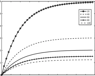
This section investigates how Ramsey fiscal policy is affected the initial level of public debt. Figure 3 shows the impulse response of the fiscal variables to a government consumption shock associated with steady-state debt levels ranging from 20 to 100 percent of GDP. In our specification, the optimal response of real public debt is to increase by thesameamount independently of its initial level. Hence, real public debt grows more for lower initial debt levels once the increase is expressed in percentage points.

Since the increase in the level of real public debt is the same, this means that all economies must raise their tax revenues by the same amount in order to finance the interest payment on the increase of the debt. Hence, tax rates increase by the same amount and have the same dynamics.

Ramsey fiscal policy is therefore independent of the initial level of debt in our specifica-tion. In response to a government spending shock, real public debt increases by the same amount independently of the initial debt level, which in turn requires an identical increase in

(15)

0 1 2 3 4 5 6 7 8 9 10 −0.18 −0.16 −0.14 −0.12 −0.1 −0.08 −0.06 −0.04 −0.02 0 Deficit as % of GDP

Years after shock

0 1 2 3 4 5 6 7 8 9 10 −3 −2.5 −2 −1.5 −1 −0.5 0 Tax

Years after shock

0 1 2 3 4 5 6 7 8 9 10 0 0.1 0.2 0.3 0.4 0.5 0.6 0.7 Consumption

Years after shock

0 1 2 3 4 5 6 7 8 9 10 −0.14 −0.12 −0.1 −0.08 −0.06 −0.04 −0.02 0 0.02 Hours

Years after shock

0 1 2 3 4 5 6 7 8 9 10 −5 −4.5 −4 −3.5 −3 −2.5 −2 −1.5 −1 −0.5 0

Nominal interest rate

Years after shock

0 1 2 3 4 5 6 7 8 9 10 −0.03 −0.025 −0.02 −0.015 −0.01 −0.005 0 0.005 Inflation

Years after shock

(16)

0 1 2 3 4 5 6 7 8 9 10 0.218 0.22 0.222 0.224 0.226 0.228 0.23 0.232

Years after shock Tax Rate 20 40 60 80 100 0 1 2 3 4 5 6 7 8 9 10 0 1 2 3 4 5 6

Years after shock

Real Public Debt

20 40 60 80 100

Figure 3: Impulse response to a one percentage point government consumption shock with different steady-state debt levels

tax rates that generates an identical increase in revenues to finance higher interest payments.

8 Fiscal Cooperation

Ramsey cooperative fiscal policy studies how fiscal policy in country 1 and in country 2 should respond to a shock so as to maximize the jointutility in the monetary union, namely the weighted average of the utility functions of the two representative citizens. We have assumed the weight of each utility function to be equal to the relative size of the country.

Under Ramsey fiscal cooperation, country 2’s fiscal policy responds to a shock in country 1 and vice versa. Figure 4 shows the impulse of variables in country 2 in response to a one percentage point increase of government spending shock in country 1, namely the same shock considered in Figure 1. The optimal fiscal response in country 2 is to raise taxes and run budget surpluses in the short run. Intuitively, the deficits of country 1 are matched by surpluses in country 2. However, the short-run increase of the tax rate in country 2 is about half the increase in country 1. Private consumption is crowded out on impact but it raises above its steady-state value thereafter. Hours worked also increase in the short run in response to the demand shock.

From the monetary union point of view it is optimal to match public deficits in country 1 to public surpluses in country 2 to avoid a large fall in bond prices that, in turn, would require an even larger tax increase in country 1. The public surpluses in country 2 reduce the net supply of bonds and help spreading the tax distortion over the monetary union.

There are two additional reasons why a shock in country 1 generates a fiscal response in country 2. One is the international transmission of shocks stemming from the fact that

(17)

0 1 2 3 4 5 6 7 8 9 10 −0.05 −0.045 −0.04 −0.035 −0.03 −0.025 −0.02 −0.015 −0.01 −0.005 0 Deficit as % of GDP

Years after shock

0 1 2 3 4 5 6 7 8 9 10 −0.05 0 0.05 0.1 0.15 0.2 0.25 0.3 0.35 Tax

Years after shock

0 1 2 3 4 5 6 7 8 9 10 −0.045 −0.04 −0.035 −0.03 −0.025 −0.02 −0.015 −0.01 −0.005 0 0.005 Consumption

Years after shock

0 1 2 3 4 5 6 7 8 9 10 0 0.005 0.01 0.015 0.02 0.025 0.03 0.035 Hours

Years after shock

Figure 4: Impulse response in country 2 to a one percentage point government consumption shock in country 1

the two countries trade extensively in goods and assets. The other reason is that monetary policy responds to union-wide shocks. As a result, the international transmission of shocks is important in our model, as it is the case in the EMU.

8.1 Ramsey Fiscal and Monetary Policy

Monetary and fiscal policy interact in a number of ways. On one side, a short-run increase in the nominal interest rate raises the cost of borrowing and depresses bond prices. The Ramsey fiscal planner will therefore rely more on raising taxes than on deficit financing of a shock. On the other hand, an increase in the labor income tax rate is likely to have a negative impact on hours worked and have inflationary consequences that, in turn, will require an increase of the nominal interest rate.

(18)

This section characterizes optimal fiscal and monetary policy. The Ramsey planner now decides not only the labor income tax but also the nominal interest rate. Our goal is to compare dynamics under Ramsey fiscal and monetary policy with the dynamics under Ram-sey fiscal and rule-based monetary policy to understand how monetary and fiscal policies interact.

Figure 5 shows the impulse responses of some macroeconomic variables under Ramsey monetary and fiscal policy and under Ramsey fiscal policy and the interest rule (21) with

φπ = 1.5 andφi = 0.9. Ramsey monetary policy reduces on impact the nominal interest rate

whereas rule-based monetary policy raises it. The Ramsey planner tolerates slightly higher inflation in order to bring a stronger expansionary response. By cutting the cost of issuing bonds, the Ramsey planner can even cut taxes in the short run to bring out an even stronger response of hours. As a result, the deficit is smaller under Ramsey monetary policy as well as the fall in private consumption.

Other studies have analyzed the response to a government spending shock in a closed economy and the impulse responses of figure 1 are in line with them. In a closed economy with a number of additional frictions, Schmitt-Grohe and Uribe (2005) find a similar dynamic response of the nominal interest rate and the tax rate, namely that they fall in impact, rise and then fall again. As a result, they also find a positive response of hours, output and inflation and a negative response of private consumption under Ramsey monetary and fiscal policies. Interestingly, the initial negative response of the nominal interest rate and the labor income tax rate is replaced by a positive one when Schmitt-Grohe and Uribe analyze simpler policy rules that, in the case of monetary policy, resemble quite closely the Taylor-type rule (21).

9 The Speed of Adjustment

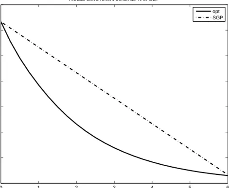
The recent reform of the SGP requires EMU member countries that have yet not achieved their medium-term objective for the budget deficit to undertake an annual adjustment of at least 0.5 percent of GDP. Figure 9 compares the optimal speed of adjustment with the mandated adjustment of the SGP. The lines in figure 9 are the budget deficits as percent of GDP under optimal fiscal policy and under the assumption that the country adjusts at the annual speed of 0.5 percent of GDP. The adjustment speed required by the SGP is lower than the optimal one and it results in budget deficits consistently higher than those stemming from Ramsey fiscal policy for over six years.

10 Conclusions

We have studied optimal fiscal policy in an economy with sticky prices that consists of two countries belonging to a monetary union. The main findings of our work can be summarized as follows. First, in response to a government spending shock, it is optimal to raise taxes and run budget deficits in the country where the shock originates; the other country finds

(19)

0 1 2 3 4 5 6 7 8 9 10 −14 −12 −10 −8 −6 −4 −2 0 2

Years after shock

Nominal Interest Rate

Rule Ramsey 0 1 2 3 4 5 6 7 8 9 10 −0.01 0 0.01 0.02 0.03 0.04 0.05

Years after shock

Inflation Rule Ramsey 0 1 2 3 4 5 6 7 8 9 10 −0.05 0 0.05 0.1 0.15 0.2 0.25 0.3 0.35 0.4 0.45

Years after shock

Tax Rate Rule Ramsey 0 1 2 3 4 5 6 7 8 9 10 0 0.02 0.04 0.06 0.08 0.1 0.12 0.14 0.16

Years after shock

Deficit as % of GDP Rule Ramsey 0 1 2 3 4 5 6 7 8 9 10 −0.02 0 0.02 0.04 0.06 0.08 0.1 0.12

Years after shock

Hours Rule Ramsey 0 1 2 3 4 5 6 7 8 9 10 −0.06 −0.05 −0.04 −0.03 −0.02 −0.01 0

Years after shock

Consumption

Rule Ramsey

Figure 5: Impulse response to a one percentage point government consumption shock under Ramsey and under rule-based monetary policy

(20)

0 1 2 3 4 5 6 0 0.5 1 1.5 2 2.5 3 3.5

Years after shock

Annual Government deficit as % of GDP

opt SGP

Figure 6: Adjustment Speed under Optimal Fiscal Policy and the SGP

it optimal to also raise tax rates that lead to budget surpluses and an improved long run equilibrium. Second, real public debt and taxes display random walk behavior. Following a government shock, for example, the optimal fiscal policy implies an increase in real debt and therefore a worsening of the net asset position of the country. Third, the optimal fiscal policy does not change with the initial level of debt.

Ramsey monetary policy is less aggressive than monetary policy implied by an interest rate rule. In response to a government spending shock, the interest rate increases when monetary policy follows an interest rate rule. On the other hand, under Ramsey monetary policy the nominal interest rate falls. This reduction of the cost of borrowing makes the fiscal response smoother and more expansionary under Ramsey monetary policy.

Our work studies optimal fiscal policy in a relatively simple setup with a representative agent and with no utility stemming from public good provision. This simple setup is justified by our focus on the stabilization part of fiscal (and monetary) policy. Fiscal policy, however, has other components we have abstracted from. Public spending on investment may improve the productivity of factors of production and therefore boost economic activity in the future, as argued by Blanchard and Giavazzi (2003). Households may care about public good provision and, more importantly, they may care differently about different public goods as some may prefer spending on national defense over spending on environmental issues or viceversa. Under this scenario, governments are partisan and electoral uncertainty biases

(21)

fiscal policy away from optimality by making governments run excessive deficits. Beetsma and Debrun (2004, 2005) argue that fiscal limits ´a la SGP help reduce such deficit bias but also reduce spending on “high-quality” outlays such as public investment and other outlays typically associated with economic reforms. Future research should incorporate these characteristics of fiscal policy and emphasize the political-economy issues related to the implementation of fiscal policy rules.

References

Aiyagari, S. Rao; Marcet, Albert; Sargent, Thomas J. and Juha Seppala. 2002. “Opti-mal Taxation without State-Contingent Debt,” Journal of Political Economy, 110(6), December, 1220-54.

Basu, Susantu and John Fernald. 1997. “Returns to Scale in U.S. Production: Estimates and Implications,” Journal of Political Economy, 105, 249-83. April.

Beetsma, Roel and Lans Bovenberg. 1998. “Monetary union without fiscal coordination may discipline policymakers.” Journal of International Economics, 45, 239–258. Beetsma, Roel and Xavier Debrun. 2004. “Reconciling Stability and Growth: Smart Pacts

and Structural Reforms,” IMF Staff Papers, 51, 3, 431-56.

Beetsma, Roel and Xavier Debrun. 2005. “Implementing the Stability and Growth Pact: Enforcement and Procedural Flexibility,” ECB Working paper,433, 1-55.

Blanchard, Olivier and Francesco Giavazzi. 2003. “Improving the SGP through a Proper Accounting of Public Investment,” working paper, MIT.

Bilbiie, Florin O., Meier, Andre and Gernot J. Muller. 2006. “What Accounts for the Changes in U.S. Fiscal Policy Transmission?” ECB working paper No. 582.

Bils, Mark and Peter Klenow. 2004. “Some Evidence on the Importance of Sticky Prices.”

Journal of Political Economy, 112.

Chari, V. V.; Christiano, Lawrence J. and Patrick J. Kehoe. 1991. “Optimal Fiscal and Monetary Policy: Some Recent Results,” Journal of Money, Credit and Banking, 23, August, 519-39.

Chari, V. V. and P. Kehoe. 2004. “On the Desirability of Fiscal Constraints in a Monetary Union,” Federal Reserve Bank of Minneapolis.

Clarida, Richard, Gal´ı, Jordi and Mark Gertler. 1999. “The Science of Monetary Policy: A New Keynesian Perspective,” Journal of Economic Literature, 37, 1661-1707.

Correia, Isabel; Nicolini, Juan P. and Pedro Teles, 2003. “Optimal Fiscal and Monetary Policy: Equivalence Results.” CEPR Discussion Papers: 3730.

Dixit, Avinash and Luisa Lambertini. 2003a. “Interactions of Commitment and Discretion in Monetary and Fiscal Policies.” American Economic Review, 93(5), December, 1522–42. Dixit, Avinash and Luisa Lambertini. 2003b. “Symbiosis of Monetary and Fiscal Policies in

(22)

Dixit, Avinash and Luisa Lambertini. 2001. “Monetary-Fiscal Policy Interactions and Com-mitment Versus Discretion in a Monetary Union.” European Economic Review,45(4-6), May, 977-87.

Eichengreen, Barry and Charles Wyplosz. 1998. “The Stability Pact: More than a Minor Nuisance?” Economic Policy,0(26), April, 65-104.

Erceg, Cristopher J.; Henderson, Dale W. and Andrew T. Levin. 2000. “Optimal Monetary Policy with Staggered Wage and Price Contracts.” Journal of Monetary Economics,

46(2), October, 81-113.

Gal´ı, Jordi. 2003. “New Perspectives on Monetary Policy, Inflation, and the Business Cy-cle,” in Advances in Economic Theory, edited by: M. Dewatripont, L. Hansen, and S. Turnovsky, vol. III, 151-197, Cambridge University Press.

Gal´ı, Jordi; Lopez-Salido J. David and Javier Valles. 2004. “Rule-of-Thumb Consumers And The Design Of Interest Rate Rules,” Journal of Money, Credit and Banking, vol. 36(4,Aug), 739-763.

Gal´ı, Jordi and Tommaso Monacelli. 2000. “Optimal Monetary Policy and Exchange Rate Volatility in a Small Open Economy.” Mimeo, Universitat Pompeu Fabra, May.

Gal´ı, Jordi and Roberto Perotti. 2003. “Fiscal Policy and Monetary Integration in Europe.” NBER Working Paper 9773.

Khan, Aubhik; King, Robert G. and Alexander Wolman. 2002. “Optimal Monetary Policy.” NBER Working Paper 9402.

Lambertini, Luisa. 2006. “Monetary-Fiscal Interactions with a Conservative Central Bank,”

Scottish Journal of Political Economy, 53(1), February, 90-128.

Levine, P. and A. Brociner, 1994, Fiscal policy coordination and EMU: A dynamic game approach, Journal of Economic Dynamics and Control,18(3/4), 699–729.

Lucas, Robert and Nancy Stokey. 1983. “Optimal Fiscal and Monetary Policy in an Economy without Capital.” Journal of Monetary Economics, 12.

Rotemberg, Julio and Michael Woodford. 1999. “Interest Rate Rules in an Estimated Sticky Price Model.” Monetary Policy Rules, Taylor, J. ed. The University of Chicago Press, 57-119.

Schmitt-Grohe, Stephanie and Martin Uribe. 2004a. “Optimal Monetary and Fiscal Policy Under Sticky Prices.” Journal of Economic Theory, 114 (2), 198-230.

Schmitt-Grohe, Stephanie and Martin Uribe. 2004b. “Solving Dynamic General Equilib-rium Models Using a Second-Order Approximation to the Policy Function.”Journal of Economic Dynamics and Control, 28, January, 755-775. September.

Schmitt-Grohe, Stephanie and Martin Uribe. 2004c. “Optimal Simple and Implementable Monetary and Fiscal Rules, ”NBER Working Papers 10253.

Schmitt-Grohe, Stephanie and Martin Uribe. 2004d. “Optimal Monetary and Fiscal Policy Under Monopolistic Competition,” Journal of Macroeconomics, 26, 183-209.

(23)

Schmitt-Grohe, Stephanie and Martin Uribe. 2005. “Optimal Fiscal and Monetary Policy in a Medium-Scale Macroeconomic Model: Expanded Version,” NBER Working paper 11417, June.

Sibert, Anne. 1992. “Government finance in a common currency area.” Journal of Interna-tional Money and Finance, 11, 567–578.

Smets, Frank and Raf Wouters. 2002. “An Estimated Stochastic Dynamic General Equilib-rium Model of the Euro Area.” ECB Working paper No. 171.

Woodford, Michael. 2000. “The Taylor Rule and Optimal Monetary Policy.” Mimeo, Prince-ton University. December.

Woodford, Michael. 2003. Interest & Prices. Princeton University Press.

Wyplosz, Charles. 2005. “Fiscal Policy: Institutions versus Rules.” National Institute Eco-nomic Review, 91, 70-84.

Wyplosz, Charles. 2006. “European Monetary Union: The Dark Sides of a Major Success.”

(24)

Appendix

A

The Ramsey Problem

The benevolent planner solves the following problem:

Lt =Et ∞ X s=t βs−t 2 X i=1 ni n

U(Ci,s−biCi,s−1, Ni,s) +λci,s[UCC, i, s−biβUC(C, i, s−1)−λi,s] +

(A.1) λτ i,s " −τi,s+ Ã 1 + UN,i,s λi,swi,s !# + λd

i,s[Ai,sNi,s−xi,sYs] +λmi,s

"

bg_i,s

1 +is

+wi,sNi,sτi,s−

bg_i,s₋₁ πs −Gi,s # + βλm i,s+1 " bg_i,s₊₁ 1 +is+1 +wi,s+1Ni,s+1 Ã 1 + UN,i,s+1 λi,s+1wi,s+1 ! − b g i,s πs+1 −Gi,s+1 # + λo

i,s[θvi,s−(θ−1)vvi,s] +λpi,s

 ₋_v_i,s_{+ ˜}_p−θ−1 i,s Ysmci,s+φβ λi,s+1 λi,s πθ s+1 Ã ˜ pi,s ˜ pi,s+1 !₋_θ₋₁ vi,s+1  ₊ λp_i,s₋₁ β  ₋_v_i,s₋₁_{+ ˜}_p−θ−1 i,s−1Ys−1mci,s−1+φβ λi,s λi,s−1 πθ s Ã ˜ pi,s−1 ˜ pi,s !₋_θ₋₁ vi,s  ₊ λpp_i,s  ₋_vv_i,s_{+ ˜}_p−θ i,sYs+φβ λi,s+1 λi,s πθ−1 s+1 Ã ˜ pi,s ˜ pi,s+1 !₋_θ vvi,s+1  ₊ λpp_i,s₋₁ β  ₋_vv_i,s₋₁_{+ ˜}_p−θ i,s−1Ys−1+φβ λi,s λi,s−1 πθ−1 s Ã ˜ pi,s−1 ˜ pi,s !₋_θ vvi,s  ₊_λmc i,s " mci,s− wi,s Ai,s # + λx i,s h

−xi,s+ (1−φ)˜pi,s−θ+φπθsxi,s−1

i

+βλx i,s+1

h

−xi,s+1+ (1−φ)˜pi,s−θ+1+φπsθ+1xi,s

i

+ +λh

i,s

h

−hi,s+ (1−φ)˜pi,s1−θ+φπsθ−1hi,s−1

i

+βλh i,s+1

h

−hi,s+1+ (1−φ)˜p1i,s−+1θ +φπsθ+1−1hi,s

i λe i,s " λi,s 1 +is −βλi,s+1 πs+1 # + λ e i,s−1 β " λi,s−1 1 +is−1 −βλi,s πs # + λb i,s " bp_i,s 1 +is +mi,s+Ci,s− bp_i,s₋₁+mi,s−1 πs

+wi,s(1−τi,s)Ni,s+hi,sYs−wi,sNi,s+

γi 2 ³ bp_i,s−¯bp_i´2+τm i,s ¸ +βλb i,s+1 " bp_i,s₊₁ 1 +is+1 +mi,s+1+Ci,s+1− bp_i,s+mi,s πs+1 +

wi,s+1(1−τi,s+1)Ni,s+1+hi,s+1Ys+1−wi,s+1Ni,s+1+

γi 2 ³ bp_i,s₊₁−¯bp_i´2+τm i,s+1 ¸¾ +

(25)

λi s · −is+ ¯i+φy µ_Y s−Y Y ¶ +φπ µ_π s−π π ¶ +φi(is−1−¯i) ¸ + βλi s+1 · −is+1+ ¯i+φy µ_Y s+1−Y Y ¶ +φπ µ_π s+1−π π ¶ +φi(is−¯i) ¸ + λπ s h −φπθ−1 s + (1−φ) ³ n1p˜11−,sθ+n2p˜12−,sθ ´ −1i+λy s[Ys−Cs−Gs],