Automatically Inferring Patterns of Resource Consumption
in Network Traf
fi
c
Cristian Estan, Stefan Savage, George Varghese
Computer Science and Engineering DepartmentUniversity of California San Diego cestan,savage,[email protected]
ABSTRACT
The Internet service model emphasizes flexibility – any node can send any type of traffic at any time. While this design has allowed new applications and usage models to flourish, it also makes the job of network management significantly more challenging. This paper describes a new method of traffic characterization that automatically groups traffic into minimal clusters of conspicuous consumption. Rather than providing a static analysis specialized to capture flows, plications, or network-to-network traffic matrices, our ap-proach dynamically produces hybrid traffic definitions that match the underlying usage. For example, rather than re-port five hundred small flows, or the amount of TCP traffic to port 80, or the “top ten hosts”, our method might reveal that a certain percent of traffic was used by TCP connec-tions between AOL clients and a particular group of Web servers. Similarly, our technique can be used to automat-ically classify new traffic patterns, such as network worms or peer-to-peer applications, without knowing the structure of such traffic a priori. We describe a series of algorithms for constructing these traffic clusters and minimizing their representation. In addition, we describe the design of our prototype system, AutoFocus and our experiences using it to discover the dominant and unusual modes of usage on several different production networks.
Categories and Subject Descriptors
C.2.3 [Computer-Communication Networks]: Network Operations—Network monitoring
Keywords
Traffic measurement, Network monitoring, Data mining
1. INTRODUCTION
The Internet is a moving target. Flash crowds, stream-ing media, CDNs, denial of service (DoS) attacks, network worms, peer-to-peer applications – these are but a few of the
Permission to make digital or hard copies of all or part of this work for personal or classroom use is granted without fee provided that copies are not made or distributed for profit or commercial advantage and that copies bear this notice and the full citation on thefirst page. To copy otherwise, to republish, to post on servers or to redistribute to lists, requires prior specific permission and/or a fee.
SIGCOMM’03,August 25–29, 2003, Karlsruhe, Germany.
Copyright 2003 ACM 1-58113-735-4/03/0008 ...$5.00.
forces that shape traffic on today’s networks. Each year, new applications and usage models emerge, and from these arise new communications patterns. This flexibility is a hallmark of the Internet architecture and can be credited with much of the Internet’s success. At the same time, this quality also brings serious challenges for network management. Un-like the traditional voice networks, which are built around a single high-level abstraction for application data transfer (“calls”), managers of IP-based networks are forced to in-ferthe type of traffic and how it relates to applications and users. Consequently, to understand and react to changes in network usage, a network manager must first analyze the bit patterns in individual packets, extract an appropriate traffic model and then reconfigure network elements to recognize that model appropriately.
To make this process feasible in practice, managers use a standard set of pre-defined patterns to identify well-known aspects of network traffic. For example, network managers frequently construct a model of application usage by clas-sifying traffic according to the IP header fields: Protocol and SrcPort. Such an analysis might determine that 90 per-cent of traffic uses the TCP protocol, 75 perper-cent of TCP traffic is for the HTTP service, 10 percent is for SMTP, 5 percent for FTP and so on. Similarly, to identify individ-ual conversations between pairs of hosts, the five tuple (Sr-cIP, DstIP, Protocol, SrcPort, DstPort), is used to impart a “flow” abstraction on traffic. These kinds of analyses, exemplified by popular monitoring tools such as FlowScan, and Cisco’s FlowAnalyzer, are a staple of modern network management [14]. However, they have two significant lim-itations when used in practice: insufficient dimensionality andexcessive detail.
While network traffic may be characterized by many dif-ferent criteria, it is easiest to aggregate traffic along one dimension at a time. Unfortunately, by aggregating traffic along any single dimension, the network manager inevitably loses any interesting, but orthogonal, structure. For ex-ample, by aggregating traffic according to an application-oriented view (i.e. Protocol and SrcPort), a network man-ager might conclude that peer-to-peer file sharing applica-tions are in wide use, when in fact a small set of hosts are responsible for most of the file sharing traffic [15]. While the network manager can expose this structure by using finer-grained representations, such as flows, she then must man-age the excessive detail contained in such a representation. Rather than identifying the file-sharing traffic concisely, the flow-oriented view decomposes it into thousands of individ-ual network transfers.
Consequently, network managers spend considerable time manually “hunting for needles” in their data – trying to un-derstand what are the real and significant sources of traffic in their network and which components of usage are changing over time. This problem is only exacerbated when there is a pressing need to understand and respond to sudden traffic spikes such as network worms or denial-of-service attacks. Moreover, automated techniques for addressing these issues – such as network pushback [11] – also require a means to identify malicious aggregates.
The focus of our work is to help automate these tasks and this paper makes four contributions in this direction. First, in Section 2 we motivate the need for a new approach to traffic monitoring that can automatically classify traffic into appropriate multi-dimensional clusters. We define a concrete and practical instance of such traffic clusters and describe a set of operations for reducing their size and in-creasing their utility. Based on this definition, Section 3 de-scribes and evaluates algorithms for cluster construction and for implementing the key operations described in Section 2. Finally, in Section 4 we describe AutoFocus, our prototype system, and in Section 5 we describe our experience using it on several production networks. At the end of our paper, we relate our efforts to previous work and then summarize our results.
2. MULTI-DIMENSIONAL TRAFFIC
CLUSTERS
While the goal of every traffic analysis method is to em-power the human operator with improved understanding, there is an inherent contradiction between the level of detail provided and the capacity of humans to absorb information: more detail can lead to a deeper understanding but makes the report harder to read – at one extreme is a bandwidth meter, at the other extreme are raw packet traces. The sim-plest solution is to report only the largest flows, so-called “top ten” reports, but this approach has a serious flaw: ag-gregates made up of many small flows can be important, but each individual flow may not be large. For example, a busy Web server might generate the bulk of the traffic, but since all of its flows are relatively small, the “top ten” re-port might only contain transfers from a nearby FTP server hosting a few large files.
Another solution is to aggregate the individual flows into a common category (e.g. by source or destination port, source or destination address, prefix or Autonomous System num-ber). However, if we chose the wrong dimension to aggregate over then we may miss the interesting characteristics of the traffic. For example, if we aggregate traffic by port num-ber, we may miss the importance of traffic generated by a denial-of-service attack using random port numbers. In this case, aggregating traffic by destination address would likely be a more useful approach.
However, in some cases there is significant information that is hidden by aggregating on anysinglefield, but is re-vealed by aggregating according to a combination of fields (multi-dimensional aggregates). For example, aggregating traffic by IP address might identify a set of popular servers and aggregating traffic by port might identify popular ap-plications, but to identify which server generates which kind of traffic requires aggregating according to two fields simul-taneously.
Our way out of this impasse is to focus on dynamically-defined traffic clusters instead of individual flows or other predefined aggregates. Our aim is to define the clusters so that any meaningful aggregate of individual flows is a traf-fic cluster. For example, a single cluster might represent all TCP client traffic originating from America Online’s net-work destined for a cluster of replicated Web servers on Google’s network. Another cluster might represent signif-icant amounts of traffic originating from a host infected by the Sapphire worm destined to random addresses at UDP port 1434. While the goal is clearly attractive, automati-cally building such clusters is quite challenging. In practice, creating effective clusters requires balancing three key re-quirements:
• Dimensionality. The dimensionality of the problem is defined by how many distinct properties are consid-ered in constructing a traffic cluster. If there is too little dimensionality then important traffic categories can be masked, while if there is too much, the compu-tational overhead of computing cluster combinations can become infeasible.
• Detail. While multi-dimensional clusters allow us to capture the structure of the traffic being analyzed, this does nothing to reduce the magnitude of data that must be evaluated – one can easily create thousands of clusters from a traffic trace. To make such data useful, a clustering algorithm must carefully prune this set to remove “unimportant” clusters and tradeoff the loss in detail for corresponding gains in conciseness.
• Utility. In the end, network managers are not merely passive observers of traffic, but are active parties who attempt to control and react to changes in traffic load and usage. Therefore, while we could construct traffic clusters using arbitrary combinations of packet header bit patterns, it is far more useful to restrict our choices to header fields that are already well-classified by net-work hardware and can therefore be acted upon.
2.1 De
fi
ning Traf
fi
c Clusters
Based on these principles, we define our traffic clusters in terms of the five fields typically used to define a fine-grained flow: source IP address, destination IP address, protocol, source port and destination port. Unlike individual flows defined by unique values for each of these fields, clusters are defined by sets of values for each of these fields. These sets can contain a single value, all possible values (we use * to denote this case) or restricted subsets of possible values.
Evaluating all possible subsets of the values for each field would have made the problem of finding all large clusters unnecessarily difficult. Instead, we use the natural hierar-chies that exist for each field. For IP addresses a cluster can be defined by prefixes of length from 8 to 32 (for individual IP addresses) or (*) for all IP addresses. For port num-bers, clusters can be defined by a particular port number (e.g. port 80) or the set of all possible values (*). Because well known ports statically allocated for services are below 1024 and ephemeral ports allocated on-demand to clients are above 1023 the set of high (>1023) port numbers and that of low (<1024) ones can also define clusters. Finally, the protocol field can take on exact values or (*).
For example, the cluster defined as (SrcIP=10.8.200.3, DstIP=*, Proto=TCP, SrcPort=80, DstPort=*) represents
Web traffic from the server with address 10.8.200.3. (Sr-cIP=*, DstIP=172.27.0.0/16, Proto=TCP, SrcPort=low, Dst-Port=high) represents TCP traffic coming from low ports and going to high ports destined to a certain prefix. Finally, (SrcIP=*, DstIP=*, Proto=ICMP, SrcPort=*, DstPort=*) represents all ICMP traffic. Notice that the first two clusters overlap with each other while the third cluster is unique.
There are many ways to further generalize the definition of traffic clusters. For example, we could define a hierar-chies based on Autonomous System number, integer ranges of port numbers, or arbitrary user-defined categories (e.g. Universities, Broadband Access, Data Centers, etc.). We could also employ heuristics such as those for identifying passive FTP and Napster traffic (that use random ports) in [14]. While these additions may provide greater value in some settings, they do not require any fundamental changes in our approach, merely a different set of aggregation criteria when constructing clusters. For the remainder of this paper we restrict our discussion to the “vanilla” cluster definitions we have described previously.
There are three advantages to this cluster definition. First, our definition is sufficiently general to capture much of the usage structure in existing applications and networks. Sec-ond, our definition is consistent with current packet clas-sifiers [8] and consequently a manager can apply controls, such as policy routing and hardware rate limiting, to the clusters we dynamically identify. Third, our definition al-lows a simple visually appealing rule-based display of clus-ters (Section 4). Finally, initial results on several distinct networks (Section 5) indicate that clusters defined in this way do identify interesting resource consumption patterns that managers care about.
Our definition of clusters satisfies two of the requirements: the need for multi-dimensional clusters (dimensionality) and field selection constrained by existing field hierarchies (util-ity). However, satisfying the remaining requirement, reduc-ing detail, requires significant additional effort.
2.2 Operations on Traf
fi
c Clusters
Atraffic reportis a list of clusters presented to a manager. It is very easy to see that even restricting ourselves to IP prefixes and very simple port ranges, that there is an expo-nential number of raw clusters. There are approximately 233 possible source IP prefixes alone! The first step in reducing this onslaught of data is to restrict the report to only in-cludehigh volumeclusters, where volume may be defined as the number of bytes or the number of packets contained in the cluster over a predefined measurement interval. While other criteria could be used to filter clusters, data volume is a categorization of inherent interest. A cluster containing 20 percent of all traffic is one that a network manager is likely to care about, while a cluster that only contains a few packets usually warrants less attention.
However, even with this restriction, the number of such clusters identified in real traces is far too large to manage. Since the precious resource is not network bandwidth or CPU cycles, but a network manager’s time, verbose and un-structured reports are not likely to be appreciated or useful. Consequently, to maximize the effectiveness of a traffic re-port, we believe that there are four essential operations that must be provided:
• Operation 1, Compute: Given a description of traf-fic as input (e.g., packet traces or NetFlow records),
compute the identity of all clusters with a traffic vol-ume above a certain threshold. This is the base oper-ation.
• Operation 2, Compress: Having found the base set of clusters, one can compress the report considerably by removing a clusterCfrom the report if clusterC’s traffic can be inferred (within some error tolerance) from that of clusterC that is already in the report. For example, if all the traffic is generated by a single high-volume connection from source S to destination D is high volume, then one can infer that the traffic sent bySis also high volume. Thus one should retain theStoDcluster for the detail it shows, and omit the Scluster as it can be inferred from theStoDcluster. Intuitively, the rule we use is to remove a more general cluster if its traffic volume can be inferred (within some error tolerance) from more specific clusters included in the report.
• Operation 3, Compare: A good way to save the manager time is to concisely show how the traffic mix changes from day to day, or week to week. Computing these deltas requires finding those high volume clusters that have changed significantly since the last report. This is trickier than it seems, because a high volume cluster on day 1 may now become low on day 2, or vice versa. Worse, more general clusters need not be larger than the sum of more specific non-overlapping clusters. Thus combining deltas (Operation 3) with compression (Operation 2) is much harder than just implementing each operation in isolation.
• Operation 4, Prioritize: Even after compressing the report and computing Deltas, it is still desirable to prioritize the elements of the report in terms of their potential level of interest to a manager. We choose to equate the interest in a cluster to what we call its unexpectedness. While there are many ways to define this metric, we chose to use a relatively unsophisti-cated approach that is easy to compute. We define unexpectedness in terms of deviation from a uniform model in which the contents of different fields is mutu-ally independent. For example, if prefixAsends 25% of the traffic and prefix B receives 40% of all traffic, then under the assumption of independence, we would expect the traffic from Ato B to be 25%*40%=10% of the total traffic. If the actual traffic from A to B is 15% of the total traffic instead of 10%, the clus-ter is tagged with a score of 150%, indicating that it is unexpectedly large by a factor of 1.5. If the traf-fic from A to B is only 6%, then it is given a score of 60%, indicating that it is unexpectedly small. The closer a score is to 100%, the more boring it is, and the less important it is to highlight to the user. This con-struction of unexpectedness is, in effect, a very simple multi-dimensional gravity model.
3. ALGORITHMS
The last section motivated four fairly abstract operations on sets of clusters. Here we describe the specific algorithms we chose to implementthese operations. These algorithms form the engine that underlies the core of our AutoFocus tool described in Section 4. Rather than directly present the
algorithms for the multi-dimensional case, we first present the simpler algorithms for the unidimensional (i.e., single field) case. Addressing this simpler case will help build in-tuition. Furthermore AutoFocus also includes in its output the simpler unidimensional results and the multidimensional algorithms use the results of the unidimensional algorithms to reduce their search space.
For some of the algorithms we also present theoretical up-per bounds on the size of the report and on the algorithm’s running time. Measurement results in the technical report version of this paper [5] show that in reality reports are much smaller than these upper bounds. Since our focus in this pa-per is maximizing information transfer to the manager, not algorithmic optimization; we believe that significantly faster algorithms that produce similar results may be possible.
In this section we use the terms dimension and field inter-changeably since each field defines a dimension along which we can classify. We usek for the number of fields. In the actual system we implementedk= 5.
The sets (i.e., prefixes in IP address fields) for each field form a natural hierarchy in terms of set inclusion. This can be described by a tree where the parent is always the smallest superset of the child. The leaves of this tree are individual values the field can take. The root is always the set of all possible values, *. The sets denoted by two nodes are disjoint unless one of the nodes is an ancestor of the other, in which case it is a superset of the other. We call the number of levels in this tree the depth of the tree (the maximum distance from the root to a leaf plus 1). We use di for the depth of the hierarchy of thei-th of thek fields.
The hierarchy for IP addresses we use in this paper has a depth of 26 that for port numbers has a depth of 3 while for the protocol field we use the simplest possible hierarchy with a depth ofd= 2.
The raw data we build our algorithms on is a simplified version of NetFlow flow records: each flow record, which we sometimes refer to as a “flow” for conciseness, has a key that specifies exact values for all five fields and two counters, one counting the packets that matched the key during the measurement interval considered and one for the number of bytes in those packets. Transforming a trace with packet headers and timestamps into such flow records leads to no loss of information from the standpoint of traffic clusters.
We use n for the number of such records. Each traffic cluster is made up of one or more flow records and the responding byte and packet counters are the sum of the cor-responding counters of the flow records it includes. Note that if a cluster contains exact values in all fields it is ex-actly equivalent to a single flow. For the rest of this section we ignore that the flow records contain two counters and work with a single counter. Our algorithms use a thresh-old H and focus on the traffic clusters that are above this threshold. We uses for the ratio between the total traffic T and the threshold s =T /H, so if H is 5% of the total traffic, thens= 20.
3.1 Unidimensional clustering
First we concentrate on the problem of computing high volume clusters on a single field, such as the source IP ad-dress. Note that even the unidimensional case is significantly more complex than traditional tools like FlowScan, in which managers define a static hierarchy by pre-specifying which subnets should be watched. By clustering automatically, we
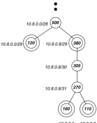
10.8.0.3 10.8.0.6 10.8.0.7 10.8.0.2 15 35 30 40 50 70 50 35 35 75 75 75 10.8.0.9 10.8.0.8 160 110 270 10.8.0.10 10.8.0.14 380 305 10.8.0.12/30 10.8.0.14/31 10.8.0.10/31 10.8.0.0/28 10.8.0.8/30 10.8.0.8/31 10.8.0.4/30 10.8.0.6/31 70 10.8.0.0/30 10.8.0.2/31 10.8.0.0/29 120 500 10.8.0.8/29
Figure 1: Each individual IP address sending traffic appears as a leaf. The traffic of an internal node is the sum of the traffic of its children. Nodes whose traffic is above H=100 (double circles) are the high volume traffic clusters. The Web server 10.8.0.12 is a large cluster in itself. While no individual DHCP address is large enough, their aggregate 10.8.0.0/29 is, so it is listed as a large cluster.
do not need to define subnets; the tool will automatically group addresses into “subnets” that contain a high volume of traffic.
We usedto represent the depth of the hierarchy andm≤ n to represent the number of distinct values of the field in thenflow records of the input.
Computing Unidimensional Clusters
Before we describe our algorithms for computing the high volume unidimensional clusters, it is useful to bound their number. Consider the IP source address. A reasonable in-tuition might be that a thresholdH of 5% of the total traf-fic restricts the report size to 20, because there can be at most 20disjointclusters, each contributing 5% of the traf-fic. Unfortunately, our definition of clusters allows clusters to overlap. Thus, if 128.50.∗.∗is a high volume cluster, then 128.∗.∗.∗is as well. Fortunately, a given source address cluster’s traffic can at most be counted in 25 other clus-ters (the number of ancestors in its hierarchy tree – we do not consider prefixes with lengths from 1 to 7). Therefore, the maximum number of high volume clusters is not 20 but roughly 20·26 = 520. In [5] we show that the size of all such reports is bounded by 1 + (d−1)s.
For the unidimensional case, we now describe the algo-rithm to do Operation 1, computing the raw set of high volume clusters. When the number of sets in the hierarchy is relatively small, for example 257 for protocol and 65539 for port numbers, we can apply a brute force approach: keep a counter for each set and traverse all nflow records while updating all relevant counters; at the end, list the clusters whose counters have exceededH.
If the number of possible values is much larger, as is the case for IP addresses, we use another algorithm illustrated by the example from Figure 1. As we go through the flow records, we first build the leaf nodes that correspond to the IP addresses that actually appear in the trace. For exam-ple, there are only 8 possible source addresses (leaves) in the trace that Figure 1 was built from. Thus, we make a pass
over the trace updating the counters of all the leaf nodes. By the end of this pass, the leaf counters are correct; we also initialize the counters of all nodes between these leaves and the root to 0. In a second pass over this tree, we can deter-mine which clusters are above thresholdH by traversing in post order (children before parents). Also, just before fin-ishing with each node, the algorithm must add its traffic to the traffic of its parent. This way, when the algorithm gets to each node its counter will reflect its actual traffic. The memory requirement for this algorithm isO(1 +m(d−1)) and it can be reduced toO(m+d) by generating the internal nodes only as we traverse the tree. The running time of the algorithm isO(n+ 1 +m(d−1)). No algorithm can execute faster thanO(n+ 1 + (d−1)s) because all algorithms need to at least read in the input and print out the result.
Compressing Unidimensional Traf
fi
c Reports
For the unidimensional case, we now describe the algorithm for Operation 2, compressing the raw set of high volume clusters. The complete list of all clusters above the thresh-old is too large and most often it contains redundant infor-mation. Even if a /8 (address prefix of length 8) contains exactly the same amount of traffic as a more specific /24 prefix, all the prefixes with lengths in between are also high volume clusters. More generally, perhaps an intermediate prefix length like /16 has a little more traffic than the /24 it includes (or the sum of the traffic of several more specific /24s already in the report) but not much more. Report-ing the /16 adds little marginal value but takes up precious space in the report. Removing the /16 on the other hand, will mean that the manager’s estimate of the /16 may be a little off. Thus we trade accuracy for reduced size. In general, define the compression thresholdC as the amount by which a cluster can be off. In our experiments we de-finedC=H. We did so to avoid unintended errors: if the manager wants all clusters aboveH, surely she realizes that the report can be off byH in terms of missing clusters of size smaller thanH. By settingC=H, we are only adding another way to be off byH. Also, settingC=H produces the following simple but appealing result.
Lemma 1. The number of clusters above the threshold in a non-redundant compressed report is at mosts.
Proof Since none of the clusters in the report is redundant, each has a traffic of at leastC=H that was not reported by any of its descendants. The sum of these differences is at mostT because each flow can be associated with at most one most specific cluster in the report and these flows make up the difference between that cluster and the more specific ones. Therefore, a report can contain at most T /H = s clusters.
If we go back to our original example for computing all clusters that send over 5% of the total traffic, we find that the number of clusters in the compressed report (assuming C=H = 5%) is at most 20 and not roughly 20·26. The compressed report corresponding to Figure 1 is in Figure 2. Note that the number of nodes retained in the report (nodes with double circles) has dropped from 7 to 4 which is actu-ally less than the 5 Lemma 1 would have predicted for the 20% threshold.
Our algorithm for computing the unique non-redundant compressed report, exemplified in Figure 2, relies on a single traversal of the tree of the high volume traffic clusters. Each
10.8.0.9 10.8.0.8 10.8.0.8/31 160 110 10.8.0.0/28 10.8.0.8/30 305 500 270 120 10.8.0.8/29 380 10.8.0.0/29
Figure 2: The clusters from the compressed re-port are represented with double circles. Node 10.8.0.8/31 is not in the compressed report because its traffic is exactly the sum of the traffic of its chil-dren. Node 10.8.0.8/30 is not in the compressed report because its traffic is within a small amount (35) of as what we can compute based on its two descendants in the report.
node in the tree maintains two counters: one reflecting its traffic and one reflecting an estimate of its traffic based on the more specific clusters included in the report. We per-form a post order traversal and decide for each node whether it goes into the report or not. We compute the node’s “es-timate” as the sum of the estimates of its children. If the difference between this value and the actual traffic is below the threshold, the node is ignored, otherwise it is reported with its exact traffic and its “estimate” counter is set to its actual traffic. This algorithm significantly reduces the size of the report while guaranteeing that all clusters of sizeH or larger can be reconstructed within errorC.
Computing Unidimensional Cluster Deltas
While compressed reports provide a complete traffic char-acterization for a given input, sometimes we are more in-terested in how the structure of traffic has changed. More specifically, the challenge is to produce a concise report that indicates the amount of the change for all the clusters whose increase or decrease in traffic is larger than a given thresh-old.
There are two ways to define the problem: by looking at the absolutechange in the traffic of clusters, or by looking at therelativechange. If the lengths of the measurement in-tervals are equal and the total traffic doesn’t change much, one can use absolute change: the number of bytes or pack-ets by which the clusters increase or decrease. However, to compare the traffic mix over intervals of different lengths (e.g. how does the traffic mix between 10 and 11 AM differ from the traffic mix of the whole day), we can only meaning-fully measure relative change and must normalize the sizes of traffic clusters so that the normalized total traffic is the same in both intervals. Thus, even if the traffic of a given cluster changed significantly, if it represents the same per-centage of the total traffic, its relative change is zero. For
the rest of this paper we assume that the we are comput-ing the absolute change or that the traffic has already been normalized.
To detect the clusters that change by more than H, we can use the full traces from each interval, but a more effi-cient algorithm can be built simply using the uncompressed reports computed earlier. Since each cluster in the uncom-pressed report is above a threshold of H, if a cluster was below H in both intervals it could not have changed by more than H overall. But operating only on the reports for the two intervals still leaves some ambiguities: we can-not be sure whether a cluster that appears only in one of the intervals and is close toH was zero in the other one and thus changed by more thanH, or was close to but belowH and thus changed by very little. Of course, if the threshold used by the input reports is much belowH, the ambiguity is reduced and we can ignore it in practice. A simple pre-processing step can provide the exact input required for the delta algorithm as follows: using reports with thresholdH for both intervals we compute the set of clusters that were aboveH in either of them and in one more pass over the trace we compute the exact traffic in both intervals for each of these clusters.
We can apply to delta reports a compression algorithm similar to that from the previous section. We decide whether to include a cluster into the compressed delta report by com-paring its actual change to the estimate based on more spe-cific clusters already reported: if the estimate is lower or larger by at least H than the actual change, the cluster is reported. Note that this can (and does) lead to putting clusters that did not change by more than the threshold into the compressed delta report. Consider the following example. The traffic from port 80 (Web) increased by more than the threshold and therefore we put it into the delta re-port. At the same time, no traffic from individual low ports changed much and the total traffic from low ports remained the same. This is possible because traffic from many low ports may have decreased slightly, thus compensating for the increase in port 80 traffic. Our compressed delta report needs to indicate that the total traffic from low ports did not change because otherwise the manager would assume that it increased by approximately as much as the Web traffic.
Lemma 2. The number of clusters in a non-redundant compressed delta report is at mosts1+s2.
Proof Each cluster in the report covers a traffic of at least H from one of the intervals that was not reported by any of its descendants. The sum of the absolute value of these differences is at mostT1+T2 (T1 is the total traffic of the
first measurement interval andT2 is the total traffic of the second one) because each flow can be associated with at most one most specific cluster in the report and the sum of the sizes of all flows is T1+T2. Therefore, there are at most (T1+T2)/H=s1+s2clusters in the compressed delta report.
While this result suggests that compressed delta reports could be double the size of compressed reports, in practice traffic changes slowly, so the deltas are much more compact than compressed reports using the same threshold.
3.2 Multidimensional clustering
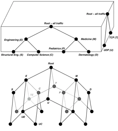
The relationships between multidimensional clusters form a more complex space defined by combining multiple
unidi-Medicine (M) Root C E UE UC U TE S T M D P Engineering (E) Structural Eng. (S) Pediatrics (P) Dermatology (D) UDP (U) TCP (T) Root − all traffic
Root − all traffic
Computer Science (C)
Figure 3: The multidimensional model combines unidimensional hierarchies (trees) into a graph. The hierarchy on the near side of the cube breaks up the traffic by prefixes; the hierarchy on the right side of the cube by protocol. For example, the node la-beled C on the near side represents the Computer Science Department, the node labeled U on the right side represents the UDP traffic and the node labeled UC in the graph represents the UDP traffic of the Computer Science Department.
mensional hierarchies. In the top of Figure 3, the closer face of the cube shows the prefix hierarchy that breaks up the traffic of a hypothetical university between the Engineering School and the Medical School, and breaks up the traffic of the Engineering School between the Structural Engineering Department and the Computer Science Department. On the right side of the cube we illustrate another hierarchy that breaks up the traffic by protocol into TCP and UDP. When we combine these hierarchies in the bottom of Figure 3 we obtain a specific type of directed acyclic graph, a semi-lattice. Nodes in this graph have up to k parents instead of just one: one parent for each dimension along which they are not defined as *. For example, node UC represents the UDP traffic of the Computer Science Department and has as parents the nodes UE (the UDP traffic of the Engineer-ing School) and C (the total traffic of the Computer Science Department). Unlike unidimensional clusters, two multidi-mensional clusters can overlap and still neither includes the other: one can be more general along one dimension, while the second can be more general along another one. For ex-ample, clusters UE and C overlap (their intersection is UC) but neither includes the other. As a result, the size of the graph is much larger than the sizes of the trees representing the hierarchies of individual fields: it is the product of their
sizes.
We use the phrase unidimensional ancestor of cluster X along dimensionito denote the cluster that is identical to X in itsith field and has wildcards in all the otherk−1 fields. This is also a unidimensional cluster along dimensioni. In our example, C is the unidimensional ancestor of UC along the prefix dimension and U is its unidimensional ancestor along the protocol dimension. We use the phrase children of cluster X along dimension ito denote the clusters that have exactly the same sets for all other dimensions and for dimensionitheir sets are one step more specific (i.e. they are children of the set used by X in the hierarchy of fieldi). For example S and C are the children of E along the prefix hierarchy and UE and TE are its children along the protocol hierarchy.
Computing Multidimensional Clusters
Our algorithm examines all clusters that may be above the threshold; for each such cluster, the algorithm examines all n flows, and adds up the ones that match. If the traffic is above the threshold, the cluster is reported, otherwise it is not. Explicitly evaluating all the clusters generated by the n flows in the input, approximately n ki=1di, is not an acceptable approach for the configurations we ran on. Therefore our algorithm restricts its search (thereby reduc-ing runnreduc-ing time) based on a number of optimizations that prune the search space.
The first optimization exploits that all the unidimensional ancestors of a certain cluster include it, so the cluster can be above the threshold only if all its unidimensional ancestors are also above threshold. We first solve thekunidimensional problems. After this, we restrict the search to those clusters that have field values appearing in each of the uncompressed unidimensional reports. Next, observe that traversal of the search space is such that we always visit all the ancestors of a given node before visiting the node itself. Thus our second optimization is to consider only clusters with all parents above the threshold. This is very easy to check because in our graph nodes have pointers to their parents. A third optimization is to batch a number of clusters when we go through the list of flow records.
Even with all three optimizations, among all our algo-rithms, this one produces the largest outputs and takes the longest to run. For example, computing both packet and byte reports with a 5% threshold takes on average 16 min-utes for a one day measurement interval, 2 minmin-utes for a one hour measurement interval and 1 minute for a five minute measurement interval using a 1 GHz Intel processor, however using a threshold of 0.5% for a one day trace it takes over 3 hours to compute the uncompressed report. We believe this algorithm can be improved significantly. In [5] we bound the number of high volume clusters in the multidimensional case bys ki=1di. While there are pathological inputs that could force the size of the output close to its worst case bound, the results for real data are much smaller.
Compressing Multidimensional Traf
fi
c Reports
For the multidimensional caseOperation 2, compression, is absolutely necessary to achieve reports of reasonable size. We first bound the maximum size of the compressed report. Lemma 3. For any traffic mix, there exists a compressed report of size at most(s ki=1di)/(max di).
COMPRESS REPORT
1 sort more specific first(cluster list) 2 foreachclusterincluster list
3 forfield= 1 to 5
4 sum[i]=add estimates(cluster.childlists[field])
5 endfor
6 cluster.estimate=max(sum[i])
7 if(cluster.traffic−cluster.estimate≥H)
8 add to compressed report(cluster)
9 cluster.estimate=cluster.traffic
10 endif
11 endforeach
Figure 4: The algorithm for compressing traffic re-ports traverses all clusters starting with the more specific ones. The “estimate” counter of each cluster contains the total traffic of a set of non-overlapping more specific clusters that are in the compressed report. The clusters whose estimate is below their actual traffic by more than the threshold H , are included into the compressed report.
Proof Letmbe the field with the deepest hierarchy (dm= max di). LetLjbe the sizes of clusters (indexed byj) that
have * in fieldm. Since each flow belongs to at most i=mdi
clusters with ∗in field m, we get
Lj ≤T i=mdi. We
can obtain any cluster by varying themth field of the cor-responding clusterj. We can compress all the clusters ob-tained from cluster j by varying field m using the unidi-mensional algorithm for field m, so by applying Lemma 1, we get that the number of clusters in the result is bound by sj = Lj/H. These reports for all j together cover all clusters, so for the total size of the report we get
Lj/H≤ s i=mdi= (s ik=1di)/(max di).
We have implemented a fast greedy algorithm for multi-dimensional compression (Figure 4). It traverses all clusters in an order that ensures that more specific clusters come before all of their ancestors (line 1). At each cluster we keep an “estimate” counter. When we get to a particular cluster we compute the sum of the estimates of its children along all dimensions (line 4) and set the estimate of the current cluster to the largest among these sums (line 6). If the dif-ference between the estimate and the actual traffic of the cluster is below the threshold (line 7), it doesn’t go into the compressed report. Otherwise we report the cluster (line 8) and set its “estimate” counter to its actual traffic (line 9). The invariant that ensures the correctness of this algo-rithm is that after a cluster has been visited, its “estimate” counter contains the total traffic of a set of non-overlapping more specific clusters that are in the compressed report. It is easy to see how this invariant is maintained: when com-puting the estimate for the cluster, for each dimension, the algorithm computes the sum of the estimates of the chil-dren of the node (cluster) along that particular dimension. Since the sets at the same level of the field hierarchy never overlap, the sets contributing to the estimates of distinct children will never overlap, so the invariant is maintained.
The compression rule allows the algorithm to consider all non-overlapping sets of more specific clusters reported when computing the estimate. Our algorithm does something
sim-pler: it only looks at the sets of non-overlapping more spe-cific clusters that can be partitioned along a dimension or another. Thusit will sometimes include clusters into the report that could have been omitted, but it will never omit a cluster that does not meet the compression criterion(i.e., is larger by more thanH than the traffic of each of the sets of non-overlapping more specific clusters in the compressed report). This is a small price to pay for the big gains in per-formance we get by performing simpler local checks. Com-puting both byte and packet compressed reports takes less than 30 seconds for a threshold as low as 0.5%.
In practice compressed traffic reports are two to three or-ders of magnitude smaller than uncompressed reports and dramatically smaller than the theoretical bound. For a thresh-old of 5% of the total traffic the average report size is around 30 clusters. This is not influenced significantly by the length of the measurement interval or the diversity of the traffic (backbone versus edge), but the size of the report is pro-portional to the inverse of the threshold. For brevity we only present in [5] our algorithm for computing compressed multidimensional delta reports, but note here that the in-teractions between compression (Operation 2) and deltas (Operation 3) are more complex than in the unidimen-sional case.
Computing “Unexpectedness”
RecallOperation 4which seeks to prioritize clusters via a measure of unexpectedness based on comparing the cluster percentage to the product of the percentages computed for each field in the cluster by itself. Computing the unexpect-edness score of a given cluster is very easy using the graph describing the relations between the high volume clusters: we only need to locate the unidimensional ancestors along all dimensions.
4. THE AUTOFOCUS TOOL
The AutoFocus prototype is an off-line traffic analysis sys-tem composed of three principal components:
• Traffic Parser. This component consumes raw net-work measurement data. Our current system uses (sampled) packet header traces as input, but it could easily be modified to accept other forms of data such as sampled NetFlow records.
• Cluster Miner. The cluster miner is the core of the tool and applies our multidimensional and unidi-mensional algorithms to compute compressed traffic reports, compressed delta reports and unexpectedness scores.
• Visual Display. The visual display component is responsible for formatting the report and construct-ing graphical displays to aid understandconstruct-ing. To im-prove user recognition of individual elements, we post-process the raw traffic report to attach salient names to individual addresses and ports. These names are generated from the WHOIS and DNS services, lists of well-known ports, as well as user-specified rules that contain information about the local network environ-ment (e.g. that a particular host is a Web proxy cache or a file server). The display component also generates a series of time-domain graphs, using different colors to identify a set of key traffic categories. These categories
can contain multiple clusters. Categories are ordered and each flow is counted against the first category it matches, traffic not falling any particular category is lumped into an “Other” category. Ideally, the cate-gories are also constructed to be representative of “in-teresting” aggregates (e.g. outbound SSL traffic from our Web servers). Currently, the user specifies these categories – typically based on examining the clusters contained in the textual report. Heuristics for auto-matically selecting these traffic categories remains an open problem, complicated by the requirement that categories be meaningful. We expect that some user involvement will always be beneficial.
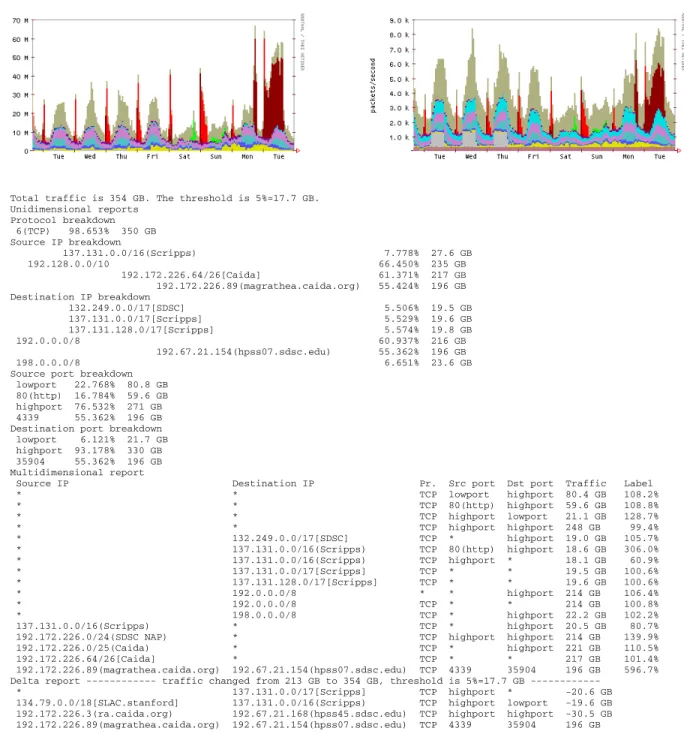
Figure 5 depicts a report generated by AutoFocus us-ing a 5% threshold on a trace recently collected from the SD-NAP exchange point. After identifying the size of the total traffic and the threshold parameters, the report pro-vides the five unidimensional compressed reports – protocol, source address, destination address, source port and desti-nation port. For example the report indicates that 66% of traffic in this trace originates from 192.128.0.0/10, however most of this traffic can be attributed to the more specific fix, 192.172.226.64/26 (owned by CAIDA). Note that pre-fixes between these two records, from /10 to /26, are com-pressed away because their traffic does not differ by more than 5% (17.7GB) from the more specific /26 prefix. Ulti-mately, an individual source IP address is responsible for the majority of this activity. The compressed multidimensional report starts with the least specific clusters (such as arbi-trary TCP traffic from servers using low ports to clients). Note that the most specific cluster shown exactly identi-fies theparticular transferthat consumed more than half of the total bandwidth. Moreover, its unexpectedness score of 596%, promptly brings it to the attention of the network administrator. Consequently, this cluster is also identified in the delta section at the end of the report. The output of AutoFocus also includes time-series plots of traffic as bytes and packets colored by the appropriate categories on two timescales: short (two days – not shown here) and long (eight days). The conspicuous spikes at each midnight are periodic backups.
The AutoFocus prototype has another feature that proved useful on a number of occasions: drilling down into indi-vidual categories. For each of the categories, we provide separate time series plots and reports that analyze the in-ternal composition of the traffic mix within that particular category.
5. EXPERIENCE WITH AUTOFOCUS
5.1 Comparison to unidimensional methods
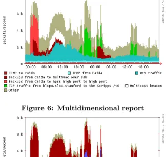
We contrast our multidimensional method with unidimen-sional analysis. Figure 6 presents a simplified version of the time domain plot generated by AutoFocus for Friday the 20th and Saturday the 21st of December 2002, while Figure 7 and Figure 8 present two unidimensional plots (see [5] for the unidimensional reports for the other fields). Be-sides compactness, our multidimensional view has the ad-vantage of making it easier to see very specific facts about the network traffic. For example the light colored “spot” between 7 AM and 2 PM on the first day is UDP traf-fic that goes to a specitraf-fic port of a specitraf-fic multicast
ad-Total traffic is 354 GB. The threshold is 5%=17.7 GB. Unidimensional reports Protocol breakdown 6(TCP) 98.653% 350 GB Source IP breakdown 137.131.0.0/16(Scripps) 7.778% 27.6 GB 192.128.0.0/10 66.450% 235 GB 192.172.226.64/26[Caida] 61.371% 217 GB 192.172.226.89(magrathea.caida.org) 55.424% 196 GB Destination IP breakdown 132.249.0.0/17[SDSC] 5.506% 19.5 GB 137.131.0.0/17[Scripps] 5.529% 19.6 GB 137.131.128.0/17[Scripps] 5.574% 19.8 GB 192.0.0.0/8 60.937% 216 GB 192.67.21.154(hpss07.sdsc.edu) 55.362% 196 GB 198.0.0.0/8 6.651% 23.6 GB Source port breakdown
lowport 22.768% 80.8 GB 80(http) 16.784% 59.6 GB highport 76.532% 271 GB 4339 55.362% 196 GB Destination port breakdown lowport 6.121% 21.7 GB highport 93.178% 330 GB 35904 55.362% 196 GB Multidimensional report
Source IP Destination IP Pr. Src port Dst port Traffic Label * * TCP lowport highport 80.4 GB 108.2% * * TCP 80(http) highport 59.6 GB 108.8% * * TCP highport lowport 21.1 GB 128.7% * * TCP highport highport 248 GB 99.4% * 132.249.0.0/17[SDSC] TCP * highport 19.0 GB 105.7% * 137.131.0.0/16(Scripps) TCP 80(http) highport 18.6 GB 306.0% * 137.131.0.0/16(Scripps) TCP highport * 18.1 GB 60.9% * 137.131.0.0/17[Scripps] TCP * * 19.5 GB 100.6% * 137.131.128.0/17[Scripps] TCP * * 19.6 GB 100.6% * 192.0.0.0/8 * * highport 214 GB 106.4% * 192.0.0.0/8 TCP * * 214 GB 100.8% * 198.0.0.0/8 TCP * highport 22.2 GB 102.2% 137.131.0.0/16(Scripps) * TCP * highport 20.5 GB 80.7% 192.172.226.0/24(SDSC NAP) * TCP highport highport 214 GB 139.9% 192.172.226.0/25(Caida) * TCP * highport 221 GB 110.5% 192.172.226.64/26[Caida] * TCP * * 217 GB 101.4% 192.172.226.89(magrathea.caida.org) 192.67.21.154(hpss07.sdsc.edu) TCP 4339 35904 196 GB 596.7% Delta report traffic changed from 213 GB to 354 GB, threshold is 5%=17.7 GB
* 137.131.0.0/17[Scripps] TCP highport * -20.6 GB 134.79.0.0/18[SLAC.stanford] 137.131.0.0/16(Scripps) TCP highport lowport -19.6 GB 192.172.226.3(ra.caida.org) 192.67.21.168(hpss45.sdsc.edu) TCP highport highport -30.5 GB 192.172.226.89(magrathea.caida.org) 192.67.21.154(hpss07.sdsc.edu) TCP 4339 35904 196 GB
Figure 5: The report for the 17th of December 2002 (one of the 31 daily reports for this trace) contains compressed unidimensional reports on all 5 fields and the compressed multidimensional cluster report using a threshold of 5% of the total traffic. In the unidimensional reports the percentages indicate the share of the total traffic the given cluster has. In the multidimensional report they indicate the unexpectedness score. Note how much smaller the delta report is than the full report.
dress. While we could manually correlate the corresponding “bright spots” from the protocol, destination prefix and des-tination port plots, the AutoFocus plot automatically iden-tifies the key usage directly. The massive spike causing the traffic surge from 12:01 AM until 3 AM the first day and the longer dark traffic cluster from 1 AM until 11 AM that day and 1 AM and to 6 AM the second day are two different types of backups. It would be difficult to disentangle them using only unidimensional plots. Since they use different
source ports (SSH versus high ports) they show up sepa-rately in the source port report, but since they come from the same source network and go to the same destination network they show up together in those plots.
5.2 Experience with analysis of traf
fi
c traces
This section presents highlights of our experience using AutoFocus to analyze traffic traces from three large produc-tion networks. While the usefulness of the insights gleaned
Figure 6: Multidimensional report
Figure 7: Unidimensional – source port
Figure 8: Unidimensional – destination network
using AutoFocus is hard to quantify, we hope that present-ing some of them will give the reader a more accurate idea of the power of our system.
Small network exchange point
Our first trace was collected from SD-NAP, a small network exchange point in San Diego, California, that connects many research and educational institutions and also connects some of them to the rest of the Internet. The trace is 31 days long and it starts on the 7th of December 2002. In addition, we were able to consult with those familiar with this network to calibrate our conclusions and receive useful feedback about out results.
When analyzing the raw reports we looked for traffic clus-ters that were large, but did not completely dominate the traffic (e.g. the cluster containing all TCP traffic is not very useful). In particular, we found that port 80 (TCP) Web traffic was so large that it was best subdivided into
four categories: Web traffic from a particular server at the Scripps Institute, Web traffic destined for clients within the Scripps /16 (Web client traffic), other traffic from port 80 and traffic to port 80. Of these, the first and second cate-gories proved to be the most interesting. Traffic from the Web server showed a clear diurnal pattern with peaks be-fore noon (sometimes a second peak after noon) and lows after midnight. It also showed a clear weekly pattern with lower traffic on the weekends and holidays. The second cat-egory (the Web clients) had similar trends, but the lows around midnight usually went down to zero and the differ-ence between weekend and weekday peaks was much larger. In retrospect, this is to be expected since the client traffic requires the physical presence of people at Scripps, while the server traffic can be driven by requests from home machines or users outside the institution.
Another interesting traffic cluster contained Web proxy traffic originating from port 3128 of a particular server at NLANR. The amount of traffic had a daily and weekly cycle, but the lowest traffic was at noon and the highest at mid-night. Using AutoFocus’ drill-down feature we were able to examine the breakdown of this traffic, which identified large clusters containing transfers to second-level caches from Tai-wan, Indonesia, Spain and Hong Kong. Evidently the traffic was driven by the daily cycle of the clients in these other time zones.
AutoFocus places the remaining non-categorized traffic into an amalgamated “Other” category. On the last day of the trace, we saw a huge sharp increase at 5:30 PM in the “Other” traffic that saturated the link followed by a sudden decrease at 11 PM. Again using the drill-down feature, we observed that this change was mostly attributable to traf-fic between two nearby universities: from UCSD to UCLA. However, traffic between these two did not appear in any other cluster over the previous 30 days. Upon investigation we determined that traffic bulge was due to a temporary net-work outage that forced traffic normally using the CalREN network to transit SD-NAP instead.
Large research institution
Our second trace was taken from the edge of a network that connects a large research institution (roughly 15,000 hosts) to the Internet. The trace is 39 days long and it starts on the 12th of December. In this case, we had access to similar although less-detailed expertise concerning the operation of the network.
Many findings for the second trace were similar to those we have described earlier, but there were some differences. We observed a series of regularly scheduled backup transfers: one from a range of machines destined to TCP port 7500 that had regular daily spikes at 11PM and 5AM followed by periods of quiescence. Another example was a regular 40GB transfer that started at 8PM on each Wednesday (usually lasting until 10AM the following morning). This activity proved to be a full backup of a large RAID array.
We observed a single large cluster containing a series of regular TCP transfers from a single host to port 5002 on three other hosts distributed around the Internet. This turned out to be a regularly scheduled network measurement experiment that was part of a distributed research activity. The most interesting result for this second trace came by looking at the breakout of the Sapphire worm [12]. This worm exploits a vulnerability of the Microsoft SQL server
Figure 9: The Sapphire/SQL Slammer worm shows up in the time series plots as a big increase in the traffic of the “Other” category around 21:30. Once we highlight the worm by putting it into a separate category, it is evident that while its traffic is significantly reduced at 22:10 when the infected internal hosts were neutralized, worm traffic persists at a lower level because of outside hosts spreading it into this network.
running on UDP port 1434 and spreads extremely aggres-sively using single 404 byte packets to infect random destina-tions. We computed the traffic reports for three hour mea-surement intervals. The time at which the worm started was apparent in the time series plot (see Figure 9). It showed up as a huge increase in the “Other” traffic category. Drilling down into the report describing that category, the worm was conspicuous: 90% of the traffic was to UDP port 1434. A quick comparison between the packet and byte reports also gave us the average packet size. Furthermore, the report readily revealed the 6 internal IP addresses that generated 80% of the traffic: these were local hosts infected by the worm aggressively trying to infect the outside world. These compromised servers were promptly neutralized by the net-work administrators. In the next three hour interval, while the traffic in the “Other” category decreased to levels simi-lar to those before the worm, still a substantial fraction of it (23%) was worm traffic. The report revealed that this was traffic originating on the outside: it consisted of incoming probes trying to infect internal hosts. We also performed an analysis of the trace with the worm traffic separated into its own category (the second plot from Figure 9). We were able to see fine details. For example some of the infected hosts did not spread their traffic uniformly over the whole address space, but focused on single /8s. This is consistent with the observation [12] that for some values of the random seed, the algorithm used by the worm to select target addresses chooses them from a limited set. This example shows once again the strength of our multidimensional approach: Auto-Focus is able to promptly bring to the network manager’s attention and describe in great detail such unexpected and unpredictable event as a worm epidemic.
While none of the traces we worked with contained mas-sive denial of service attacks, we believe that AutoFocus would bring them to the attention of the network operator the same way it showed the worm. The victim of the at-tack (whether it is an individual IP address or a prefix) will show up in the report with a very large number of packets (or bytes depending on the type of attack). Furthermore, the attack will reveal the protocol used by the attack and possibly the port number if it is kept constant. If the source address is faked at random from the whole IP address space, the report will not associate any particular source address with the attack traffic hitting the victim. However, if for some reason (e.g. egress filtering at the site the attack
orig-inates from), the source addresses are restricted to a certain prefix (or a small number of prefixes), the report will identify these, thus facilitating prompt and specific response.
We presented the output of AutoFocus to network man-agers of the first two networks we had traces from. Their reactions were very positive. It was easy for them to un-derstand the output. They appreciated the intuitiveness of the time series plots, the large amount of information they convey and the ease with which the traffic reports and the drill-down feature provided them more detailed information when they needed it. The managers of both networks ex-pressed interest in widely deploying our tool.
Backbone
A third trace we looked at was captured in August 2001 from an OC-48 backbone link and is 8 hours long. We looked at traffic reports for one hour measurement intervals. The re-ports reveal that around two thirds of the bytes on the link come from TCP port 80 and around one third come from high ports. The report also revealed that around one third of the traffic was from high ports to high ports. This is con-sistent with the behavior of peer to peer traffic. Through the unexpectedness scores, the report revealed some further facts that seemed surprising at first. There were specific source and destination prefixes where the Web traffic rep-resented almost all of the traffic. One explanation for the prefixes that send almost only Web traffic is the clustering of Web servers in Web hosting centers or server farms. The prefixes that receive almost exclusively Web traffic could be organizations with many Web clients whose internal policy prohibits the use of peer to peer applications.
6. RELATED WORK
FlowScan [14] is a package by Dave Plonka used for vi-sualizing network traffic. It uses NetFlow [13] data to give detailed information about the traffic by breaking it down in a number of ways: by the IP protocol; by the well-known service or application; by IP prefixes associated with “local” networks; or by the AS pairs between which the traffic was exchanged. There are many other applications that pro-duce similar breakdowns of the traffic such as CoralReef [1] or the IPMON project [2] based on packet traces instead of NetFlow data. In [6] Estan and Varghese present algo-rithms that automatically and efficiently identify large clus-ters, once the definition of clusters is fixed. In terms of
our terminology, these reports display traffic clusters along predefineddimensions.
There are methods for reducing the size of the raw data describing the traffic mix in a way that does not preclude future analyses: through sampling [4] or sketches [7]. While our method also produces a very compact summary of the traffic mix, its primary purpose is not to be used by further analyses, but to convey a description of the traffic to the human operator.
The problems we are solving are related to classical clus-tering [10], but are different in that we use the space defined by the field hierarchies instead of a Euclidian space. An-other problem, finding association rules [3], requires finding frequent item sets in high dimensional data, and is a well studied problem in data mining. The two important differ-ences between these two problems are: 1)Most approaches to association rules do not use hierarchies. A notable ex-ception is Han and Fu [9] who use asinglehierarchy across all fields unlike our use ofseparatehierarchies for each field. 2)Our compression rules were crucial to the effectiveness of AutoFocus. To the best of our knowledge, no algorithms for association rules use compression rules similar to ours.
7. CONCLUSIONS
Managing IP-based networks is hard. It is particularly complicated by not understanding the nature of the appli-cations and usage patterns driving traffic growth. In this paper, we have introduced a new method for analyzing IP-based traffic,multidimensional traffic clustering, that is de-signed to provide better insight into these factors. The nov-elty of our approach is that it automatically infers, based on the actual traffic, a traffic model that matches the dominant modes of usage. Unlike previous work, our algorithms can analyze traffic along multiple different “dimensions” (Srource address, Destination address , Protocol, Source port, Des-tination Port) at once, and yet be able to use compression to map results from this multidimensional space into a con-cise report. In essence, our approach exploits the locality created by particular modes of usage.
In addition to developing these algorithms, we have em-bodied them in the AutoFocus analysis system. We have developed a Web-based user interface to allow managers to explore clusters across multiple time-scales and to drill down to explore the contents of any clusters of interest. Our pre-liminary experiences with this tool have been extremely pos-itive and we have been able to identify unusual traffic pat-terns that would have been considerably harder to identify using conventional tools. Moreover, we have received posi-tive feedback from network mangers who have quickly been able to appreciate the benefits of our approach.
Finally, note that AutoFocus, as described in this paper, automatically extracts patterns of resource consumption in asingle intervalof time based on the traffic log of asingle link. The natural generalization would to extend AutoFocus to automatically extract patterns of resource consumption across timeand across space. While AutoFocus currently provides a visual display across a limited number of peri-ods, it would be useful to doautomatictime-series analyses across large time periods using compressed clusters as a new and parsimonious basis for such analysis. Similarly, extend-ing AutoFocus to detect resource consumptionacross space would allow managers to detect geographical patterns within the network. We leave these generalizations for future work.
8. ACKNOWLEDGMENTS
We would like to thank Vern Paxson and Jennifer Rexford for the many discussions that led to the clarifying the con-cept of traffic clusters. We would also like to thank David Moore and Vern Paxson for help with the evaluation of the AutoFocus prototype. Support for this work was provided by NSF Grant ANI-0137102 and the Sensilla project spon-sored by NIST Grant 60NANB1D0118.
9. REFERENCES
[1] Coralreef - workload characterization.
http://www.caida.org/ analysis/ workload/. [2] Ipmon - packet trace analysis.
http://ipmon.sprintlabs.com/ packstat/ packetoverview.php.
[3] R. Agrawal, T. Imielinski, and A. Swami. Mining association rules between sets of items in large databases. InProceedings of the ACM SIGMOD, 1993. [4] N. Duffield, C. Lund, and M. Thorup. Charging from
sampled network usage. InSIGCOMM Internet Measurement Workshop, November 2001.
[5] C. Estan, S. Savage, and G. Varghese. Automatically inferring patterns of resource consumption in network traffic. Technical report CS2003-0746, UCSD. [6] C. Estan and G. Varghese. New directions in traffic
measurement and accounting. InProceedings of the ACM SIGCOMM, 2002.
[7] A. Gilbert, Y. Kotidis, S. Muthukrishnan, and M. Strauss. Quicksand: Quick summary and analysis of network data. Dimacs technical report, 2001. [8] P. Gupta and N. Mckeown. Packet classification on
multiple fields. InProceedings of the ACM SIGCOMM, 1999.
[9] J. Han and Y. Fu. Discovery of multiple-level association rules from large databases. InProceeding of VLDB, 1995.
[10] T. Hastie, R. Tibshirani, and J. Friedman. The elements of statistical learning. Springer, 2001. pages 453-479.
[11] R. Mahajan, S. Bellovin, S. Floyd, J. Ioannidis, V. Paxson, and S. Shenker. ACM SIGCOMM CCR, Vol 32, No. 3, July 2002.
[12] D. Moore, V. Paxson, S. Savage, C. Shannon, S. Staniford, and N. Weaver. The spread of the sapphire/slammer worm. Technical report, January 2003.http://www.caida.org/ outreach/ papers/ 2003/ sapphire.
[13] Cisco netflow.http://www.cisco.com /warp /public /732 /Tech /netflow.
[14] D. Plonka. Flowscan: A network traffic flow reporting and visualization tool. InProceedings of USENIX LISA, 2000.
[15] S. Saroiu, K. Gummadi, R. Dunn, S. Gribble, and H. Levy. An analysis of internet content delivery systems. InProceedings of OSDI, 2002.