Linking Cross-Sectional and Aggregate Expected Returns

=

=

Working Paper

=

Linking Cross-Sectional and Aggregate Expected Returns

Serhiy Kozak

University of Michigan

Shrihari Santosh

Ross School of Business Working Paper

Working Paper No. 1257

November 2014

This work cannot be used without the author's permission. This paper can be downloaded without charge from the Social Sciences Research Network Electronic Paper Collection:

Linking Cross-Sectional and Aggregate Expected

Returns

∗

Serhiy Kozak§, Shrihari Santosh‡

November 19, 2014

Abstract

We propose a one state variable ICAPM that rationalizes the size, value, and mo-mentum “anomalies” observed in stock returns. Our main insight is that differential covariance with news about future market discount rates drives the observed cross-sectional variation in expected returns. We find that in response to an increase in expected future market discount rates, large, growth, and recent losers company stocks outperform small, value, and recent winner stocks, respectively. Our interpretation is that such an increase in discount rates represents “bad” news for the representative investor, increasing his marginal utility of wealth. We further show that ignoring this state variable leads to drastic underestimation of the equilibrium price of “level risk” measured using bond returns. An augmented model which adds a “level” factor jointly prices both stock and bond returns.

∗_{We thank John Cochrane, Eugene Fama, Stefano Giglio, Valentin Haddad, Lars Hansen, John Heaton,}

Bryan Kelly, Ralph Koijen, Diogo Palhares, Harald Uhlig for helpful comments and suggestions.

§_{Ross School of Business, University of Michigan. Email: [email protected].} ‡_{R.H. Smith School of Business, University of Maryland. Email: [email protected].}

1

Introduction

The logic of Merton(1973) suggests there exists a representation for the stochastic discount factor1 _{which is a linear combination of the return on the aggregate wealth portfolio and}

state variables which capture changes in the investment opportunity set and “outside income” (non-tradable wealth)2_{. We propose and test an equilibrium model in which shocks to risk}

aversion (sentiment) generate time-varying expected equity returns. We find support for the model’s prediction that such shocks represent “bad” news for the representative investor and manifest in the cross-section of expected asset returns.

We find that augmenting the one-factor CAPM3 _{with a single additional factor, the}

shock to expected future excess market returns, is sufficient to rationalize the cross-section of expected returns of portfolios formed on size, book-to-market ratio, and recent performance (momentum). Since the CAPM completely fails in fitting the cross-section of portfolio sorts we analyze, the success of our model comes entirely from the expected market return factor. This result is similar toCampbell and Vuolteenaho(2004) but with an important difference. Instead of the typical VAR (vector auto-regression) approach, we use future realized returns to proxy for expected future returns (see Section 2.4). This provides a consistent estimate of expected returns under any information set. Both approaches yield consistent results but under different assumptions. Our methodology produces a very different cross-sectional patterns in factor loadings. We find that growth stocks and large firm stocks outperform value stocks and small firm stocks, respectively, in response to an increase in market expected returns.

The pattern in loadings we find results in an opposite conclusion about the compensation an investor requires for bearing the risk of time-varying expected returns. We conclude that an increase in the expected market return corresponds to a drop in the investor’s utility and hence an increase in his marginal utility of wealth. This implies the investor is willing to pay in order to eliminate this risk from his portfolio. In Appendix A we solve a general equilibrium model that delivers exactly this prediction. In the model, expected market returns are high when the representative investor’s risk aversion is high. These states of the world correspond to times of high marginal utility.

The second contribution of our paper is decomposing the average return differential between 1_{Also called a state-price density. Equivalently, no arbitrage implies the existence of a present-value}

function and of an equivalent martingale measure.

2_{Under loose restrictions, even with trading constraints, the absence of arbitrage implies the existence of}

a stochastic discount factor,Mt+1, such that the relationship 1 =Et[Mt+1Ri,t+1] holds for all assetsSkiadas

(2009, Chapter 1)

Figure 1: Covariances of stock portfolios and bonds with the expected returns factor Portfolio # 1 2 3 4 5 ×10-5 0 0.5 1 1.5 2 ”Large” ”Small” Cov(Re

i,t,λt) of Portfolios Formed on ME

(a) Portfolios formed on Market Equity

Portfolio # 1 2 3 4 5 ×10-5 0 0.5 1 1.5 2 2.5 ”Growth” ”V alue” Cov(Re

i,t,λt) of Portfolios Formed on BE/ME

(b) Portfolios formed on Book-to-Market

Portfolio # 1 2 3 4 5 ×10-5 0 1 2 3 4 ”Losers” ”W inners” Cov(Re

i,t,λt) of Portfolios Formed on Prior2-12 Ret

(c) Portfolios formed on Prior 2-12m Return

Maturity (years) 3 4 5 6 7 ×10-6 0 5 10 15 20

Cov(Rei,t,λt) of zero-coupon Treasury Bonds

(d) Zero-coupon Treasury Bonds

long and short term government bonds into a large positive return differential due to loadings on “level risk” (change in long-term yields) and a large negative return differential due to loadings on our expected market return factor. These net to a slightly upward sloping term structure of expected bond returns. Koijen et al.(2010) find a similar decomposition of bond risk premia using time-varying expectedbond returns instead of stock returns. Figure 1

shows the loadings of bonds and portfolios formed on size, book-to-market, and prior 1-year return on our expected return factor. Large stocks, growth stocks, recent losers, and long-term bonds have higher covariance with innovations in the expected excess market return than small stocks, value stocks, recent winners, and short-term bonds, respectively. These patterns are consistent with a “flight-to-quality” interpretation where effective investor risk aversion rises, stock prices fall, bond prices rise, and “good” companies outperform “bad” companies.

Finally, we document that returns on the Fama-French factors smb, hml, and mom

are useful forecasters of the future market excess return, significant both statistically and economically. In our sample from 1963 to 2010, the three combined greatly outperform the

dividend price ratio, D_{/P, in terms of R}2_{. This confirms the spreads in covariances seen in}

Figure 1are of economically relevant magnitudes, aleviating concerns that our asset pricing

exercise is simply a regression of “noise on noise.”

2

The Model

2.1

Specification

FollowingDuffie and Epstein (1992a), we define a stochastic differential utility by two prim-itive functions, f(Ct, Jt) : R+ ×R → R and A(Jt) : R → R. For a given consumption

process C, the utility process J is the unique Ito process that satisfies the stochastic differ-ential equation, dJt= −f(Ct, Jt)− 1 2A(Jt)kσJ,tk 2 dt+σJ,tdZt, (1)

whereσJ,tis anR2-valued square-integrable utility-”volatility” process,Jtis the continuation utility forC at timet, conditional on current information,f(Ct, Jt) is the flow utility,A(Jt) is a variance multiplier that penalizes the variance of the utility “volatility”kσJ,tk ≡σJ,tσ

0

J,t, and Zt is a vector of shocks. A pair (f, A) is called an aggregator. We use a Kreps-Porteus (Epstein-Zin-Weil) aggregator, defined as

f(C, J) = δ ρ Cρ−Jρ Jρ−1 = δ ρJ " _C J ρ −1 # (2) A(J) = −α J, (3) where ρ = 1− 1

ψ and ψ is the elasticity of intertemporal substitution; δ is a subjective discount factor, and α is the risk-aversion parameter.

We consider a simple endowment with a dividend process given by:

dD

D =gtdt+σDdZ

where gt is the mean consumption growth,

dg =φg(¯g−g)dt+σgdZ.

We further extend the utility specification when the parameter α is stochastic,

This parameter can be interpreted as either time-varying risk aversion (Campbell and Cochrane

(1999),Dew-Becker (2011)) or time-varying ambiguity aversion with respect to model

spec-ification (Drechsler (2013), Hansen and Sargent (2008))4_.

Finally, agent’s wealth evolves according to:

dW

W = (θλ+r−C)dt+θσRdZ

where θ is the share invested in the risky asset, λ is the excess return on the risky assets, r

is the risk-free rate.

2.2

Solution

Market clearing requires C =D, W =P, and θ = 1. For simplicity, we further assume that the elasticity of intertemporal substitution is equal to unity. We solve the Hamilton-Jacobi-Bellman equation corresponding to the above problem in the Appendix A.

Theorem 1. Equilibrium SDF corresponding to the problem in equations (1), (2), (3), and (4) is given by: dΛ Λ = −rdt−αdRM −(α−1)|{z}aα <0 σαdZ−(α−1) ag |{z} >0 σgdZ (5)

where RM is the return on the market portfolio, aα and ag are constants provided in the

Appendix A. When risk aversion is higher than 1, the price of risk-aversion risk is negative.

Equity Risk premium is given by

λ =λ0 +α×σDσ

0

D

where λ0 is a constant defined in the Appendix A. Finally, the risk-free rate is:

r=g−λ.

Proof. See Appendix A.

Theorem 2. The price of the (market) discount rate risk is negative when investor’s risk aversion is higher than unity. Investors dislike assets that pay off poorly in states when the discount rate is high, and command high risk premium on those assets.

4_{Variability in α generates time-varying prices of risk in the model. Our main results survive if we}

model time-varying quantity of risk (through time-varying volatility of consumption growth) instead and are therefore not exclusive to the preference specification chosen.

Proof. The result follows immediately from the fact that the coefficientaα in (5) is negative,

aα <0 (see Appendix A).

Theorem 3. Given the results in Theorem 1, the three-factor model holds:

Re_i,t = α×covt−1 Re_i,t, Re_M,t+ag(α−1)×covt−1 Re_i,t, dg (6) + (α−1)aα×covt−1 R_i,te , dλ where Re

i,t is the excess return on any test asset, ReM,t is the excess return on the market portfolio, dλ are shocks to the equity risk premium, and dg are shocks to the growth rate. The term in square brackets is negative for all plausible parameter values.

Proof. See Appendix A.

2.3

Unconditional Pricing

We further proceed with the discrete version of the model and definerxi,t+1 as the log return

on an assetiover time periodt →t+1. When instanteneous excess returnsRe_i,t are normally distributed, corresponding discrete-time excess returns rxi,t+1 are log-normally distributed.

The model above is specified conditionally with “shocks” as factors. With two assump-tions, we derive an unconditional representation in terms of “levels”.

Assumption 1. Covariances with market and expected returns factorsciM ≡covt(rxi,t+1, rxM,t+1), ciλ≡covt(rxi,t+1, λt+1), and variances Vi =vart(rxi,t+1) are constant in time.

Our goal is to capture time variation in Sharpe ratios. Empirical evidence that links conditional volatilities and conditional means is weak (Welch and Goyal,2008). We therefore, use this assumption to focus on time variation in Sharpe ratios that is driven entirely by variation in expected returns.

Assumption 2. Expected log market excess returns λt+1 = Et+1rxM,t+2 follow an AR(1)

process.

This assumption, while quite restrictive, serves primarily the purpose of deriving closed-form solutions and quantifying the effects discussed below. It allows us to capture persistence in the risk premium while keeping the model very tractable. The assumption is similar in na-ture to those made in the literana-ture, which typically assume that the vector of state variables follows a VAR(1) process (see, for example, Campbell (1996), Campbell and Vuolteenaho

Assumption 3. Consumption growth rate is constant, σg = 0.

Assumption 3 serves solely for expositional purposes in this chapter and will be relaxed

inSection 4.

Theorem 4. Given Assumption 1, Assumption 2, Assumption 3, and conditional model in

Eq. 6, we obtain the following linear pricing relation:

∀i, t : E(rxi,t+1) + Vi 2 = cov(rxi,t+1, rxM,t+1)× ˆ δM (7) + cov(rxi,t+1, λt+1)×δˆλ

where ˆδM and δˆλ are two constant unconditional prices of market and expected returns risk, respectively. Section B.2 derives the link between these prices and the conditional ones in

Appendix, Eq. 23.

Proof. Refer to the proof of a more generalTheorem 9 with the arbitrary number of factors and risk prices in Appendix, Section B.2.

Two aspects about this relation are worth emphasizing. First, all moments in the formula are unconditional and hence can be easily estimated using time-series regressions. Second, the formula involves the covariances withlevels rather than shocks. This result is an implication of homoskedasticity and the AR(1) structure imposed above.

2.4

Expected Returns Factor

2.4.1 Using Future Realized Returns

The unconditional model in Eq. 7 involves the expected return factor λt+1 which is not

directly observable by an econometrician. Empirical literature that faces this issue typi-cally uses the residual from predictive regressions instead. Campbell(1996), Campbell and

Vuolteenaho(2004) uses the VAR approach with macroeconomic and financial variables that

have been shown to be good forecasters of expected returns and thus changes in investment opportunity set. This approach narrows the information set that is used to make predictions about future returns and therefore can be potentially biased. Moreover, the information that is being used is limited to a small set of forecasters that have limited ability in forecasting returns.

We employ a novel methodology designed to circumvent the issue. We use future realized returns as an unbiased estimator of current risk premia required by investors. Future realized

returns as an estimate of expected returnsrxM,t+2 =Et+1rxM,t+2+εt+2 is indeed an unbiased

estimator, since for any information set Ft+1 at timet+ 1, Et+1(εt+2) = Et+1(εt+2|Ft+1) = 0

True (population) conditional covariances are also equal

covt(rxi,t+1, rxM,t+2) = covt(rxi,t+1, Et+1rxM,t+2)

and thus an unbiased and consistent estimator of the covariance on the RHS is also an unbiased and consistent estimator of the covariance on the LHS. See Section B.4 for a more formal argument.

Our empirical approach allows us to test the model without directly estimating expected market returns. We require a restrictive AR(1) assumption, but we make no assumptions about investors’ information set. Instead, our approach is based on the agent’s ability to forecast returns rather than econometrician’s. Unlike previous work, we do not rely on any forecasting regressions.

2.4.2 Moving Average of Future Realized Returns

One issue with using one period ahead realized returns is that the signal-to-noise ratio of such proxy is very low. If expected returns are persistent, we could cumulate sufficiently long series of future returns in order to improve the ratio. There is an obvious trade-off here: increasing the length of the cumulative sum will improve the signal-to-noise ratio at a decreasing rate. We will determine the horizon length empirically in later sections.

We now show that the cumulative sum of future realized returns can be used as a proxy for market risk premium in Eq. 7.

Theorem 5. When the expected returns factor is measured over long horizon, the uncondi-tional relation in Eq. 7 still holds, with the new prices of risk that are a linear transform of the ones in Eq. 7:

∀i, t : E(rxi,t+1) + Vi 2 = cov(rxi,t+1, rxM,t+1)× ˜ δM (8) + cov(rxi,t+1, λt+1:t+T)×δ˜λ

where λt+1:t+T = Et+1rxM,t+2:t+T+1 denotes expected market returns (risk premia) starting

market and expected returns risk, respectively. Section B.2 in the Appendix derives the link between these prices and the conditional ones in Eq. 6 and Eq. 26.

Proof. Refer to the proof of a more generalTheorem 10with an arbitrary number of factors and risk prices in Appendix, Section B.2.

In the case when the moving average of future returns is used as an estimator of the expected market returns factor, we can still show its unbiasedness. See Section B.2.1 for more details.

2.5

Price of Expected Returns Risk

We now make the following assumption that will allow us easily compare the sign on price of expected returns risk in conditional and unconditional models.

Assumption 4. Price of the expected returns (discount rate) risk is constant, var(δλ,t) = 0.

This assumption states that the time-variation in expected returns is driven exclusively by the price of market risk. This implies that the expected return on a long-short portfolio of two assets that have the same loading on the market factor is not time-varying.

Assumption 4 delivers the following result:

Theorem 6. When Assumptions 1, 2, and 4 hold, the sign of the price of expected returns risk is preserved: sign{E[δλ,t]}=sign n ˜ δλ o

where δλ,t is the price of expected returns risk in conditional model (6) andδ˜λ is the price of expected returns risk in either of conditional models in (7) or (8).

Proof. See the proof in Appendix, Section B.3.

2.6

Empirical Relation

Equipped with the results in Theorem 4 and Theorem 5, we proceed with approximating the unconditional relation inEq. 8to facilitate the empirical tests in the following Section 3.

Section B.5 in the Appendixshows, that with daily data, the unconditional pricing relation

inEq. 8 can be approximated by the following relation:

∀i, t: ERe_i,t+1 = cov(rxi,t+1, rxM,t+1)×δ˜M (9) + covrxi,t+1,ˆλt+1:t+T

where Re i ≡

Ri

Rf is the level of excess returns and ˆλt+1:t+T ≡ rxM,t+2:T =

PT

j=2rxM,t+j. In deriving this relation, we use the fact that future realized returns can be used as an unbiased and consistent estimate of market risk premia (see Eq. 27).

All the variables in Eq. 9 are observed by an econometrician. We can use the level of excess returns,Re

i, on the LHS, and the covariances of log excess returnsrxi with the market

rxM and the future realized excess returns, rxM,t+2:T =PTj=2rxM,t+j on the RHS.

In theAppendix,Section 3.4 we compare the empirical specification inEq. 9to a similar one in Campbell and Vuolteenaho(2004).

3

Empirical Link Between Cross-Sectional and

Aggre-gate Expected Returns

We estimate and test the expected return relation ofEq. 9using two sets of test assets. The first is the canonical 25 portfolios formed by a two-way sort of firms on market capitalization (SIZE) and book-to-market ratio (BE/ME), available at Ken French’s website 5_.

Lewellen et al.(2010) highlight a key issue in estimating and testing asset pricing models. When the test assets have a strong factor structure that captures much of the time-series variation as well as the cross-sectional variation in expected returns, a spurious model with many factors may still produce a remarkably good cross-sectional fit as long as the spurious factors are correlated with the “true” factors. This result is not due to sampling varia-tion; it holds in population. A solution they propose is to add assets which increase the “dimensionality” of the test asset space.

Therefore, in addition to the canonical 25 portfolios sorted on size and book-to-market ratio, we construct an alternative set of test assets. We include fifteen portfolios consisting of five value-weighted quintile portfolios each from independent sorts on size, book-to-market ratio, and momentum (PRIOR) 6_{. Fama and French (2008) show that sorting firms based}

on prior performance produces a reliable spread in average returns subsumed by neither the size effect or the book-to-market effect. Furthermore, the momentum factor, MOM (Mark M. Carhart,1997), is nearly uncorrelated with the size factor, SMB, and is negatively corre-lated with the book-to-market factor, HML (Fama and French, 1996). Therefore, including momentum sorted portfolios as test assets makes it decidedly more difficult for a model to fit the cross-section of expected returns. Our preferred estimation uses these fifteen portfolios; for robustness and for comparison with the literature, we perform all estimation and testing on the Fama-French 25 portfolios as well.

5

http://mba.tuck.dartmouth.edu/pages/faculty/ken.french/data_library.html

Following the spirit of Merton (1973) and the continuous-time model in Section 2, we use portfolio returns measured at daily frequency7_{. All returns are measured over the period}

July 1963 to December 2010. Though monthly returns are available going back to 1927, we choose to use the shorter sample of daily returns. Using daily returns reduces the approxi-mation error due to linearization of the exponential function that we rely on in deriving the estimation equation.

As noted in Campbell and Vuolteenaho (2004), “July 1963 is when COMPUSTAT data become reliable and because most of the evidence on the book-to-market anomaly is obtained from the post-1963 period”. Furthermore, in the pre-1963 sample, the “CAPM explains the cross-section of stock returns reasonably well” (Campbell and Vuolteenaho, 2004). Since inflation estimates are not available daily (and inflation is not well measured even at monthly frequency (Cecchetti,1997), we use only excess log returns, which, by construction, are real returns.

As a proxy for the excess return on the wealth portfolio, rxm,t, we use RmRf, the excess return on the value-weight portfolio of all common equity traded on the NYSE, AMEX, and NASDAQ. Of course the standard critique applies that there exist many assets, both traded (foreign securities) and non-traded (real-estate, human capital) that are not included in this portfolio (Roll, 1977). As discussed above, we construct λe_t = PH

i=1rxm,t+i. For our preferred specification, we set H = 126 trading days, or one-half year. Though the theory of

Section 2.4 implies the model should fit for all choices ofH, finite length of the historic data series means that increasing H comes with a loss of precision in estimating Covrxi,t,λe_t

. Our results are quantitatively robust across various choices of H, from 3 months to 2 years.

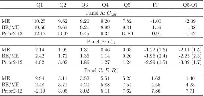
Table 1 below shows the estimated covariances of asset returns with the factors. Panel

A shows Cov(rxi,t, rxm,t) with GMM standard errors in parentheses. Quintile 1 represents large firms, growth firms, and recent losers in relation to the dimensions, size, book-to-market, and momentum, respectively. Analogously, Quintile 5 represents small firms, value firms, and recent winners. The column to the right of Quintile 5 represents the Q5-Q1 spread portfolio. The last column give the estimates for the canonical Fama-French factors, SMB, HML, and MOM. The covariances match the well known pattern in market betas.

Panel B reports Covrxi,t,λe_t

for the same portfolios. In all three dimensions (size, book-to-market, and momentum),Covrxi,t,λe_t

decreases from left to right. That is to say, when the “risk premium”,λt, rises, small stocks are expected to fall more than large stocks, value stocks are expected to fall more than growth stocks, and recent winners are expected to fall more than recent losers. Though realized returns in place of expected returns produces consistent and unbiased covariances estimates, they will be less precisely estimated due to

Table 1: Covariances Q1 Q2 Q3 Q4 Q5 FF Q5-Q1 Panel A: Ci,M ME 10.25 9.62 9.26 9.20 7.82 -1.00 -2.39 BE/ME 10.66 9.63 9.21 8.99 9.31 -1.59 -1.38 Prior2-12 12.17 10.07 9.45 9.34 10.80 -0.91 -1.42 Panel B: Ci,λ ME 2.14 1.99 1.31 0.46 0.03 -1.22 (1.5) -2.11 (1.5) BE/ME 2.42 1.71 1.36 1.14 0.20 -1.96 (2.4) -2.23 (2.3) Prior2-12 4.82 3.02 1.86 1.27 1.24 -2.29 (1.5) -3.02 (1.7) Panel C:E[Re_i] ME 2.94 5.11 5.52 5.51 5.23 1.63 1.40 BE/ME 2.48 3.71 4.20 5.88 7.54 4.55 4.23 Prior2-12 -2.19 3.05 3.02 5.11 7.62 7.86 7.71

Notes: This table shows covariances and annualized mean returns estimated over 1963:07:01-2010:12:31. Panel A lists the covariances of portfolio returns with the market return,Ci,M. Panel B depicts the covariances of portfolio returns with the expected returns factor, Ci,λ. Panel C shows the the expected excess returns on each portfolio, E[Re

i]. The column "FF" represent the Fama-French factors,smb,hml, andmom. Moving-block bootstrap t-statistics in parentheses.

the extra noise present in realized returns. Still, the covariances of the spread portfolios with λe are statistically significantly different from zero and the covariances follow a reliable

pattern, suggesting that we are not just “regressing noise on noise.”

The model in Section 2 suggests these covariances could result from a “flight-to-quality” phenomenon, where the overall risk premium rises and the risk premium on “low quality” assets rises by even more. When risk aversion rises, demand for all risky assets falls, in-creasing their risk premia. Our model is only one such motivation for time-varying expected returns. Indeed, as noted in (Shefrin, 2008, Chapter 30.3.3), the stochastic discount factor in a habit formation model (Campbell and Cochrane, 1999) is of the same general form as one based on a model of investor sentiment. Both deliver time-varying expected returns through an effectively time-varying risk-aversion parameter for the representative agent. We choose to directly model time-varying risk aversion. As we discuss below, the negative sign of

δλ, suggests that even if these covariances are produced sentiment driven “flight-to-quality” episodes, these are likely to be amplifications of fundamental shocks so that the risk-premium rises during aggregate “bad times”.

Panel C shows the sample average returns, which are monotonically increasing from left to right across quintiles, consistent with the well known size, value, and momentum premia. Panels B and C suggest a strong relationship between Covrxi,t,λe_t

Figure 2: Univariate fit Cov1Re i,t, P126 i=1R e M,t+i 2 ×10-5 0 1 2 3 4 5 E [ R e]i ( an n u al iz e d % ) -4 -2 0 2 4 6 8 me1 me2 me3 me4 me5 bm1 bm2 bm3 bm4 bm5 m1 m2 m3 m4 m5

E[R] vs covariance with risk premium, 126 day MA

(a) Quintile Portfolios

Cov1Re i,t, P126 i=1R e M,t+i 2 ×10-5 -2 -1 0 1 2 3 E [ R e]i ( an n u al iz e d % ) 0 2 4 6 8 10 12 1,3 1,4 1,5 2,1 2,2 2,3 2,4 2,5 3,1 3,2 3,3 3,4 3,5 4,1 4,2 4,3 4,4 4,5 5,1 5,2 5,3 5,4 5,5

E[R] vs covariance with risk premium, 126 day MA

(b) Fama-French 25 Portfolios

Notes: The left plot shows sample values ofE[rix,t] vsCov

rxi,t,eλt

for the 15 quintile portfolios: 5 size (me), 5 book-to-market (bm) and 5 momentum (m) sorted portofios. The plot in the right panel depicts same results for the 25 Fama-French portfolios.

be clearly seen in Figure 2. Figure 2 (a) plots sample values ofE[rix,t] vsCov

rxi,t,λe_t

for the 15 quintile portfolios. Figure 2 (b) is the same plot for the 25 Fama-French portfolios. The graphs confirm the suspicion that Covrxi,t,λe_t

and E[rix,t] line up fairly well in the cross-section of assets, suggesting an additional risk factor that captures the size, value, and momentum effects.

3.1

Estimation Results

We estimate risk price vector δ = [δM δλ]

0

using GMM with a prespecified block-diagonal weighting matrix Cochrane (2001, Chapter 11.5). It is equivalent to the standard two-stage estimation procedure. Covrxi,t,λe_t

and Cov(rxi,t, rxM,t) are estimated in the first stage by just-identified GMM, which yields the standard formulas for sample covariance. In the second stage, we minimize the mean-squared model pricing errors of the test assets. This is equivalent to and OLS regression of sample mean returns on the covariances estimated from the first stage. In addition to our two-factor ICAPM, we estimate the Sharpe-Lintner CAPM and well as the Fama-French model, augmented with the mom (momentum) factor

of Mark M. Carhart (1997). For comparison, all models are written and estimated in terms

of covariances instead of regression βs. Below is a summary of the pricing equations of the relevant models, where δs are interpreted as risk prices (coefficients in the SDF):

2-Factor ICAPM:E[R_ie] = Ci,MδM +Ci,λδλ 2-Factor ICAPM (free intercept): E[R_ie] = α+Ci,MδM +Ci,λδλ

CAPM, Restricted: E[R_ie] = Ci,MδM

4-Factor FF, Unrestricted: E[R_ie] = α+Ci,MδM +Ci,smbδsmb+Ci,hmlδhml+Ci,momδmom 4-Factor FF, Restricted: E[R_ie] = Ci,MδM +Ci,smbδsmb+Ci,hmlδhml+Ci,momδmom

whereCi,X ≡ Cov[rxi,t, Xt].

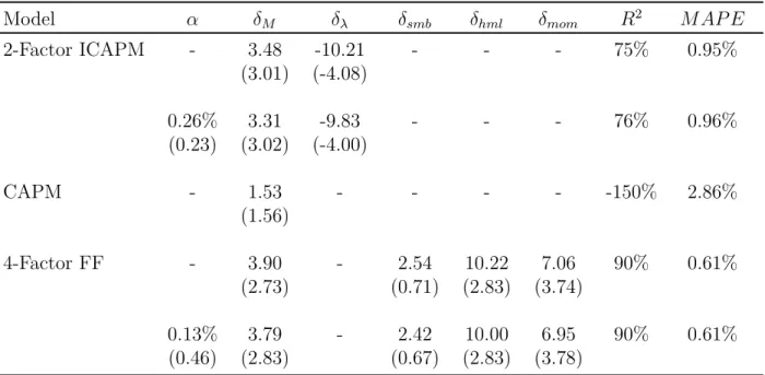
Estimated risk prices are given inTable 2along with sampleR2_{and mean absolute pricing}

errors8_{. Quantitatively, our two-factor ICAPM fits the cross-section of average returns nearly}

as well as the augmented 4-factor Fama-French model. The estimated intercept is nearly zero, both statistically and economically. Though Covrxi,t,λe_t

is not very well estimated for any individual test asset, the cross-sectional spread in covariances is strong enough to yield precise estimation of δλ. H0 : δλ = 0 is rejected for all conventional significance levels. Covariance with the expected return factor is able to capture a large portion of the cross-sectional variation in average returns due to the size, book-to-market, and momentum effects. Standard errors are calculated using the moving block bootstrap methodology (Joel L. Horowitz, 2001) and are consistent across various choices of block size.

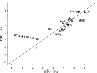
The cross-sectional fit of the ICAPM and 4-factor Fama-French models are given graph-ically in Figure 3. The graphs plot model implied average excess returns on the horizontal and sample average returns on the vertical axis. The 45◦ line represents a model with perfect in-sample fit (100% R2).

3.2

The Sign of

δ

Campbell and Vuolteenaho (2004) perform a similar pricing exercise but with different

em-pirical methodology and theoretic motivation. They find a positive price of expected returns risk, though the estimate isn’t statistically significant. From our estimation, the probability that the price of risk is positive is P[δλ >0] = 0.002% (one-sided t-test ofH0 :λ≥0 easily

rejects the null). The alternative approaches therefore reach very different conclusions. We find that growth stocks and large firm stocks outperform value stocks and small firm stocks, respectively, in response to an increase in market expected returns, opposite to the pattern in Campbell and Vuolteenaho (2004). The different pattern in loadings produces a different conclusion about the compensation an investor requires for bearing the risk of

8_{For the 4-factor model, we don’t impose the GLS restriction that the model exactly prices the factors.}

Table 2: Risk Price Estimates Model α δM δλ δsmb δhml δmom R2 M AP E 2-Factor ICAPM - 3.48 -10.21 - - - 75% 0.95% (3.01) (-4.08) 0.26% 3.31 -9.83 - - - 76% 0.96% (0.23) (3.02) (-4.00) CAPM - 1.53 - - - - -150% 2.86% (1.56) 4-Factor FF - 3.90 - 2.54 10.22 7.06 90% 0.61% (2.73) (0.71) (2.83) (3.74) 0.13% 3.79 - 2.42 10.00 6.95 90% 0.61% (0.46) (2.83) (0.67) (2.83) (3.78)

Notes: This table shows premia estimated from the 1963:07:01-2010:12:31 for the two-factor ICAPM, the CAPM, and the augmented Fama-French model. The test assets are value-weighted quintile portfolios sorted on ME, BE/ME, and Prior2-12. αis annual-ized and "-" indicates that the intercept is restricted to zero. MAPE is average absolute pricing error, annualized. Moving block bootstrap t-statistics are in parentheses

time-varying expected returns. We conclude that an increase in the expected market return corresponds to a drop in the investor’s utility and hence an increase in his marginal utility of wealth. This implies the investor is willing to pay in order to eliminate this risk from his portfolio, as predicted by our model. In contrast, Campbell and Vuolteenaho (2004) find that an investor is willing to pay to increase his exposure to this risk.

3.3

Factor Mimicking Portfolio

The two-stage OLS procedure for estimating stochastic discount factors suffers from many problems related to samples size and factor structure in the covariance of test asset returns.

Lewellen et al. (2010) highlight these concerns and offer some suggestions:

1. Increase the dimensionality of the test assets relative to the dimension of the SDF.

2. Impose theoretic restrictions: “zero-beta rates should be close to the risk-free rate, the risk premium on a factor portfolio should be close to its average excess return”. This is essentially using GLS instead of OLS with the factor included as a test asset.

3. Report GLS R2 since (a) it “is completely determined by the factor’s proximity to the minimum-variance boundary ... but the OLS R2 can, in principle, be anything”

Figure 3: Performance of the ICAPM and 4-Factor Fama-French models d E[Re i](%) -2 0 2 4 6 8 E [ R e]i ( % ) -2 0 2 4 6 8 S H M smb hml mom me1

me2 me3 me5me4

bm1 bm2 bm3 bm4 bm5 m1 m2 m3 m4 m5 2 FACTOR ICAPM

Actual vs Predicted Mean Excess Ret. (Annualized), Restricted intercept

d E[Re i](%) -2 0 2 4 6 8 10 E [ R e]i ( % ) -2 0 2 4 6 8 10 S H M smb hml mom me1 me2me3me4me5

bm1 bm2bm3 bm4 bm5 m1 m2 m3 m4 m5 Fama-French 4-Factor

Actual vs Predicted Mean Excess Ret. (Annualized), Restricted intercept

Notes: 2-Factor ICAPM with restricted intercept on the left, and 4-factor Fama-French with restricted intercept on the right. m1-m5 correspond to momentum quintile portfolios (losers to winners). bm1-bm5 correspond to book-to-market quintiles (growth to value). me1-me5 correspond to size quintiles (large to small). smb, hml, and mom are the canonical Fama-French-Carhart factors. S, H, and M are 5-1 quintile spread portfolios.

and (b) “in practice, obtaining a high GLSR2 _{represents a more stringent hurdle than}

obtaining a high OLS R2_.”

4. Report confidence intervals for the cross-sectional R2.

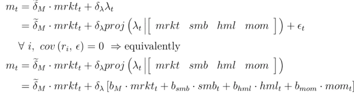
We already addressed issue (1) by having only one factor to “explain” three dimensions of average returns. Table 2 shows that estimates with and without restrictions on the zero-beta rate are nearly identical. Since our expected return factor is not an excess returns, we cannot directly include it as a test asset and check the restriction in (2). We can however, include a maximally correlated (mimicking) portfolio, i.e., regress the factor on the space of excess returns and use the fitted values. As shown in Cochrane (2001, Ch. 4), this yields identical OLS estimates of covariances, risk prices, pricing errors, and R2_{. Because}

our test assets are highly correlated, in small sample the mimicking portfolio will have unrealistic extreme long/short positions. To mitigate concern of overfitting, we alternatively construct λb_t = proj λt h mrktt smbt hmlt momt i

. This is the linear combination of the four Fama-French-Carhart factors which has maximal correlation with our original expected return factor. Since it is an expected return we can include it as a test asset and use GLS methods.

If the 2-factor ICAPM is literally true we can derive the following restriction on the SDF loadings, assumingprojλt

h mrktt smbt hmlt momt i

(including other assets doesn’t improve model fit9_). mt=δe_M ·mrkt_t+δ_λλ_t =δe_M ·mrkt_t+δ_λproj λt h mrkt smb hml mom i +t ∀ i, cov(ri, ) = 0 ⇒equivalently mt=δe_M ·mrkt_t+δ_λproj λt h mrkt smb hml mom i =δe_M ·mrkt_t+δ_λ[b_M ·mrkt_t+b_smb·smb_t+b_hml·hml_t+b_mom·mom_t]

The unrestricted four-factor SDF ismt =δM·mrktt+δsmb·smbt+δhml·hmlt+δmom·momt. If the 2-factor model is strictly true, then we should have δM = δe_M +δ_λ ·b_M and δ_i =

δλ ·bi for i ∈

n

smb hml mom o. Table 3 shows the implied and direct coefficients on

h

mrkt smb hml mom i in the SDF. The unrestricted coefficient on SMB is smaller

than the ICAPM implied value and the coefficient on MOM is larger than its implied value. The implied and direct coefficients on HML and Market are nearly identical. This is a manifestation of the αs (pricing errors) seen in the left panel of Figure 3. SMB has a lower average return than predicted by it’s covariance with λ and MOM has a positive ICAPMα. Since SDF weights are proportional to average returns when the factors are uncorrelated10

the ICAPMαs translates directly into the difference SDF coefficients. Still, it is reassuring that the restriction isn’t drastically violated.

Table 3: SDF Restriction

Restricted ZB-rate Unrestricted ZB-rate

Implied 4-Factor Implied 4-Factor

Market 4.13 3.90 3.94 3.79

SMB 4.90 2.54 4.72 2.42

HML 10.67 10.22 10.28 10.00

MOM 5.97 7.06 5.75 6.95

Notes: Implied coefficients for market are eδM +δλ·bM where δsare from the first row of

Table 2 and bM is from proj λt

mrkt smb hml mom . The remaining implied

coefficients areδi=δλ·bi withδλ andbi from the same source.

With the factor mimicking portfolio, we can address points (2) and (3) above. For the remainder of this section, we treat the mimicking portfolio as the factor and address OLS vs

9_{This assumption is approximately true in the data.} 10_{Market, SMB, HML, and MOM are nearly uncorrelated.}

GLS11_{. GLS restricts the model to exactly fit the market and the mimicking portfolio’s}

aver-age in-sample returns, ignoring pricing errors on other assets. Table 4 shows the estimated SDF using both. E[rM] andE[rλ] are the model implied annualized expected excess returns on the market and mimicking portfolios, respectively. For GLS these are, by construction, equal to annualized sample averages.

The results are similar across methods. In particular, the model implied expected returns on the two factors (market and λ mimicking portfolio) are similar for OLS and GLS. This addresses point (2) fromLewellen et al.(2010). The GLSR2 is mechanically lower than OLS

R2 but not substantally so. Bootstrap simulation rejects the null of R2 = 0 with p≈0.1%. Recall from Table 2 that the CAPM has a negative R2 due to the restricted zero-beta rate and the well known issue that average returns among these assets are negatively correlated with market betas. For comparison, the 4-factor GLS R2 _{is 79% (not shown).}

Table 4: GLS Estimation δM δλ E[rM] E[rλ] R2 M AP E OLS 3.30 -10.25 3.26 -8.01 72% 0.91% (2.86) (-3.81) GLS 3.78 -12.26 3.46 -9.58 62% 1.03% (2.90) (-4.54)

Notes: OLS estimates are from the standard two-step FM procedure. GLS restricts the model to exactly fit the market and the mimicking portfolio’s average in-sample returns, ignoring pricing errors on other assets. E[rM] andE[rλ] are the model implied annualized expected excess returns on the market and mimicking portfolios, respectively. For GLS these are, by construction, equal to annualized sample averages.

3.4

Campbell-Shiller Decomposition

Assumption 2implies that the expected returns factor can be any finite linear combination of expected future returns. In particular, it can beP∞

j=1ρjrt+1+j from the return decomposition given in Campbell and Shiller (1988) . Our empirics do not uniquely identify which one it is.

11_{When only a subset of test assets are used to construct the mimicking portfolio, there is no guarantee}

that estimated risk prices, etc will remain unchanged. The ICAPM R2 _{drops from 73% to 69% and risk}

prices, δs, are similar (±10%). We ignore sampling uncertainty in bSM B, bHM L, bM OM when reporting test statistics using the factor mimicking portfolio. This likely does not bias our results greatly since the Newey-West t-statistics onbSM B, bHM L, bM OM are between 2 and 3.

We now compare our model to a similar one inCampbell and Vuolteenaho(2004).

Camp-bell and Vuolteenaho (2004) starts with exploiting the Campbell and Shiller (1988)

decom-position: rt+1−Etrt+1 = (Et+1−Et) ∞ X j=0 ρj∆dt+1+j − (Et+1−Et) ∞ X j=1 ρjrt+1+j = NCF,t+1−NDR,t+1

where NCF denotes news to future cash flows and NDR denotes news about future discount rates.

By relying on homoskedasticity assumption and linear approximations, Campbell(1993) derives an approximate discrete-time version of Merton(1973) ICAPM:

Et(ri,t+1)−rf,t+1+ σ2 i,t 2 = γ×covt(ri,t+1, rM,t+1−EtrM,t+1) (10) + (1−γ)×covt(ri,t+1,−NDR,t+1) = γ×covt(ri,t+1, NCF,t+1) − covt(ri,t+1, NDR,t+1)

In Theorem 5 we showed that the sum of future returns over arbitrary horizon can be

used as an expected returns factor. In fact, it can be easily shown that the statement holds for any weighted sum as well with market risks being scaled by a constant. In this way, the sum of discount rates in Eq. 10, P∞

j=1ρjrt+1+j, is directly comparable to our expected returns factor factorλ. The formulation (10) therefore is similar to the conditional model in

Eq. 6. It implies however a positive price of risk on discount rate factor (which is a scaled version of our expected returns factor with positive scaling factor).

Eq. 10 can be rewritten in terms of risk prices inTable 2:

Et(ri,t+1)−rf,t+1+ σ_i,t2

2 = δM ×covt(ri,t+1, NCF,t+1)

+ (δλ−δM)×covt(ri,t+1, NDR,t+1) (11)

The essence of Campbell and Shiller(1988) decomposition is that unexpected stock mar-ket returns could be mechanically decomposed into a positive cash-flow news component and a negative discount-rate component, resulting in positive and negative betas, respectively. Further, Campbell and Vuolteenaho (2004) find that with Epstein-Zin (or power utility)

preferences, CAPM does not hold because the discount rate effect in Eq. 11 is weakened as compared to the CAPM (which holds with exponential utility, for instance). The effect is not, however, fully reversed: the price of cash-flow risk is still positive and the price of the discount-rate risk is negative. In this paper we find that the discount-rate effect is, in fact, greatly amplified when investor’s risk aversion increases in bad states of the world. Table 2

shows that the loading on the discount-rate risk, δλ, in presence of the market returns as a second factor in the SDF is significantly negative. The price of the discount-rate risk in

Eq. 11, δλ−δM, is therefore also strongly negative and higher in magnitude than the price of the cash-flow risk.

4

Pricing Bonds

Figure 4: Pricing Bonds

d E[Re i](%) -6 -4 -2 0 2 4 6 8 E [ R e]i ( % ) -6 -4 -2 0 2 4 6 8 S H M smb hml mom me1

me2 me3 me5me4

bm1 bm2bm3 bm4 bm5 m1 m2 m3 m4 m5 B2 B3 B4 B5 B6 B7 2 FACTOR ICAPM

Actual vs Predicted Mean Excess Ret. (Annualized), Restricted intercept

Notes: We plot the fitted and sample mean values of expected returns in the modelEq. 8. Test assets include the stock portfolios we used before as well as 5 bonds with maturities from 3 to 7 years, labeled B3-B7, respectively.

Whereas there are numerous papers which explore risk premia separately for equities and fixed income securities, few study these important assets in a unified framework12_{. We extend}

our analysis to include risk-free government bonds and interest rate risk.Figure 4 illustrates that the unconditional model in Eq. 8 fails to price bond excess returns of maturities from 3 to 7 years. Pricing errors are big and the slope is completely wrong. Clearly, the market

and expected returns factors are not sufficient to explain the risk compensation required for holding these securities.

We use Eq. 6 to motivate a third factor – the growth rate of the economy. The factor helps price bonds and stocks jointly. To proxy for the changes in the growth rate of the economy, we use the return on a long-maturity government bond. The yield on a long-term bond is related to the “level” factor in bonds, which has been shown to to be the only priced factor in the cross-section of nominal bonds (Cochrane and Piazzesi, 2008).

The extended model from Section 2 is:

Et(rxi,t+1) +

1 2σ

2

t(rxi,t+1) = covt(rxi,t+1, rxM,t+1)×δM,t + covt(rxi,t+1, λt+1)×δλ,t

+ covt(rxi,t+1, rxB,t+1)×δB,t (12) where rxB is the excess return on a long maturity bond. With the same assumptions as before, the model conditions down as follows:

Theorem 7. Given Assumption 1 and Assumption 2 and conditional model in Eq. 12, we obtain the following linear pricing relation:

∀i, t : E(rxi,t+1) + Vi 2 = cov(rxi,t+1, rxM,t+1)× ˆ δM (13) + cov(rxi,t+1, λt+1)×δˆλ + cov(rxi,t+1, rxB,t+1)×δˆB (14) whereδˆM ,δˆλ, andδˆB are three constant unconditional prices of market, expected returns, and bond risk, respectively. Section B.2 derives the link between these prices and the conditional ones in Operationalizing the Model.

Proof. This is a straightforward application of Theorem 9 in Operationalizing the Model,

Section B.2with two factors (market and bond) and zero price of bond risk.

Theorem 5 carries over to this case in a natural fashion:

Theorem 8. When the expected returns factor is measured over long a horizon, the uncon-ditional relation in Eq. 13 still holds, with the new prices of risk that are a linear transform of the ones in Eq. 13:

∀i, t : E(rxi,t+1) + Vi 2 = cov(rxi,t+1, rxM,t+1)× ˜ δM (15) + cov(rxi,t+1, λt+1:t+T)×δ˜λ + cov(rxi,t+1, rxB,t+1)×δ˜B (16) where λt+1:t+T = Et+1rxM,t+2:t+T+1 denotes expected market returns (risk premia) starting

one period ahead for T ≥1 periods, δ˜M ,δ˜λ, and δ˜B are three constant unconditional prices of market, expected returns, and bond risk, respectively. Section B.2 in the Operationalizing

the Model derives the link between these prices and the conditional ones in Eq. 12.

Proof. Refer to the proof of a more generalTheorem 10with an arbitrary number of factors and risk prices in Operationalizing the Model, Section B.2.

UsingTheorem 8 andSection B.5 in theOperationalizing the Model we can show in the same way as in Section 2.6that the following approximate relation holds:

∀i, t: ERe_i,t+1 = cov(rxi,t+1, rxM,t+1)×δ˜M (17) + covrxi,t+1,ˆλt+1:t+T

×δ˜_λˆ

+ cov(rxi,t+1, rxB,t+1)×δ˜B where Re_i ≡ Ri

Rf is the level of excess returns and ˆλt+1:t+T ≡rxM,t+2:T =

PT

j=2rxM,t+j. With these results in hand, we proceed with empirical tests of the model in Eq. 17.

5

Bond Risks and Risk Premia

5.1

“Level” factor

Most popular term structure models feature factors typically labelled “level”, “slope”, and “curvature”Ang and Piazzesi(2003),Diebold and Li(2006),Diebold et al.(2005),Litterman

and Scheinkman (1991). In these models, the level factor induces parallel shifts in the

log-yield curve. In the estimated affine term structure model of Cochrane and Piazzesi

(2008), unconditional expected bond excess returns are described by Erx(_ti₊₁) = δB ×

covrx(_ti₊₁) ,(Et+1−Et)levelt+1

13_{. The single factor driving expected returns is the shock}

to the “level” of yields. 13_rxi

By construction, the yield on a hypothetical bond of infinite maturity is proportionate to the level factor. Approximating the long-end of the yield curve to be flat we can write

lnP_t+1T−1_/PT t = T −1 T yT_t −yT_t+1−1 ≈ T −1 T yLT_t −y_tLT₊₁ where PT

t is the price of a T year bond at time t, and ytLT is the log yield-to-maturity of a “long-term” bond at time t. The left hand side is the log return on the long-term bond and the right hand side is a multiple of the change in the level factor (change in the long-term yield). This shows that the return on a long-term bond is essentially perfectly negatively correlated with the level factor.

Written in terms of shocks we have,

(Et+1−Et) h lnP_t+1T−1_/PT t i ≈ (Et+1−Et) _T −₁ T y_tLT −yLT_t+1

where we have equated the unexpected return on the long-term bond with the shock to the level factor. The model of Cochrane and Piazzesi(2008) can be recast as

Erx(_t+1i) = δe_B×cov

rx(_ti₊₁) ,(Et+1−Et)r(t+1LT)

.

Since the model is written in real terms but we only observe nominal bond returns, we substitute14 _rx(LT)

t+1 , the excess return on the long-term bond, in place of r (LT) t+1 , yielding Erx(_tn₊₁) = δe_B×cov rx(_ti₊₁) ,(Et+1−Et)rx (LT) t+1 = δe_BC_n,B (18)

5.2

Data

We use zero-coupon treasury yields from Gürkaynak et al. (2006) (GSW), which provides a daily constant maturity yield curve from 1961 onward. Though the data are smoothed, the yields are usually very close to the unsmoothed yields derived using the methodology

of Fama and Bliss (1987) and “for many purposes the slight smoothing in GSW data may

make no difference” (Cochrane and Piazzesi, 2008). The advantage of GSW yields is the daily observation frequency, which we have argued inSection 3is important to our empirical

strategy. Prior to 1971, the GSW yields only include maturities up to seven years. Post 1971 they includes maturities to 30 years, though there is some question of the reliability of the very long maturity yields. To match the timing of our stock data, we use maturities up to seven years, starting in 1963.

To construct daily zero-coupon bond returns from the GSW yields, we must interpolate between the given maturities. We use linear interpolation though this is technically incon-sistent with the functional form used by GSW. For daily (or even monthly) returns, this introduces negligible error since the GSW function is smooth and the weight given to the nearest whole year maturity is essentially 1 (actually 251/252). Finally, we must choose how to deal with timing. We use the convention of 252 trading days per year and treat each trad-ing day as betrad-ing 1 “day” after the previous tradtrad-ing day. This means that we have essentially eliminated weekends and trading holidays from the calendar. This introduces measurement error in the returns that is reduced as the measurement horizon increases (from daily to monthly to quarterly, etc). Excess returns just subtract the log return on a one month t-bill, the same procedure we use for stock excess returns.

5.3

Estimating the price of “level risk”

With daily excess log bond returns in hand, we estimate the model of using the same two-stage procedure ofSection 3.1. δe_B is estimated to be 3.6. The cross-sectionalR2 is 95% with

an annualized mean absolute pricing error of 0.09%. Figure 5shows graphically the good fit of the model.

In the context ofEq. 8, we argue that δe_B, the price of “level risk”, is commonly

underes-timated when usingEq. 18 and bond excess returns. It is a classic case of “omitted variable bias”15_{. Eq. 8 and the results of Section 3.1 suggest at least two such missing variables,}

Ci,λ = 106×Cov h rx(_t+1i) , Et Pk i=1rxM,t+i i

and Ci,M = 106×Cov

h

rx(_ti₊₁) , rxM,t+1

i

. Table 5

shows Ci,B, Ci,λ and Ci,M across maturities. First note that Ci,M ≈ 0 for all maturities. More importantly, ∀i, Ci,λ ≈ 1.4Ci,B. Cross-sectionally, corr(Ci,B, Ci,λ) ≈ 1. Since we know Section 3.1 that δλ 6= 0, the univariate level model suffers greatly from omitted vari-ables bias. Using the estimate ofδλ = 10.3 , a back-of-the-envelope calculation suggests the true δB = 3 + 1.4×10.3 = 17.4. In other words, the required compensation for bearing level risk is much higher than is estimated from a univariate model of bond expected returns. Treasury bonds, in addition to loading positively on level risk, also provide investors a hedge against increases in the expected return on stocks. Thus, bonds earn lower average returns than in the hypothetical economy where the expected market return is constant.

Figure 5: d E_[Re i](%) 0.2 0.4 0.6 0.8 1 1.2 1.4 E [ R e]i ( % ) 0.2 0.4 0.6 0.8 1 1.2 1.4 B2 B3 B4 B5 B6 B7

SINGLE FACTOR BOND MODEL (COCHRANE-PIAZESSI) Actual vs Predicted Mean Excess Ret. (Annualized), Restricted intercept

Table 5: Covariances 2Y 3Y 4Y 5Y 6Y 7Y Ci,B 0.29 0.60 0.92 1.22 1.51 1.78 Ci,λ 0.51 0.92 1.29 1.63 1.95 2.26 Ci,M 0.01 0.03 0.07 0.12 0.17 0.24 Ci,B = 105×Cov h rx(_t+1i) ,(Et+1−Et)rx (LT) t+1 i Ci,λ = 105×Cov h rx(_t+1i) , Et ΣkirxM,t+i i Ci,M = 105×Cov h rx(_t+1i) , rxM,t+1 i

This intuition is formalized by estimating the 3-factor ICAPM given by Eq. 15. Table 6

gives estimated risk prices (δs) from the following models:

2-Factor ICAPM: E[Re_i] = Ci,MδM +Ci,λδλ Univariate Level Risk: E[Re_i] = Ci,BδB

3-Factor ICAPM: E[Re_i] = Ci,MδM +Ci,λδλ+Ci,BδB where Ci,X ≡ Cov[rxi,t, Xt]

Table 6: Risk Price Estimates Model δM δλ δB R2 M AP E 2-Factor ICAPM 3.48 -10.21 - 2% 1.75% (3.01) (-4.03) Level Risk - - 3.01 94% 0.07% (1.21) 3-Factor ICAPM 3.10 -9.60 15.12 88% 0.73% (2.84) (-3.97) (3.47)

Notes: This table shows premia estimated from the 1963:07:01-2010:12:31 for the 2 ICAPM (estimated using stock portfolios), the Level Risk model (estimated using bond returns), and the 3-factor ICAPM (estimated using both stocks and bonds). Model intercepts are restricted to zero. MAPE is average absolute pricing error, annualized. Moving block bootstrap t-statistics are in parentheses

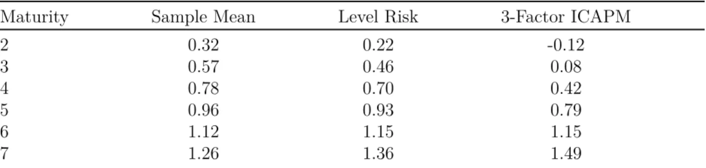
Table 7: Bond Expected Returns

Maturity Sample Mean Level Risk 3-Factor ICAPM

2 0.32 0.22 -0.12 3 0.57 0.46 0.08 4 0.78 0.70 0.42 5 0.96 0.93 0.79 6 1.12 1.15 1.15 7 1.26 1.36 1.49

Notes: Annualized percent returns by maturity.

. All models are estimated with the intercept restricted to zero. The 2-factor ICAPM is estimated using only the stock portfolios from Section 3 and hence the risk price estimates are the same as in Section 3.1. The univariate Level Risk model is estimated using only the bond excess returns. The 3-factor ICAPM is estimated using all assets, stock portfolios as well as bonds. Estimated values for δM and δλ are essentially unchanged in the 3-factor ICAPM (relative to the 2-factor estimates). TheR2 _{of the 2-factor ICAPM is so low because}

bonds are included as test assets though they are excluded from the estimation of risk prices

(see Figure 4). Importantly, δB in the 3-factor ICAPM is ≈16 3. This is similar to the

back of the envelope prediction given above.

Table 7gives annualized percent returns by maturity in sample, implied by the univariate

Level Risk model, and implied by the 3-factor ICAPM. Both models imply as larger term premium (spread between long and short maturity average returns) than is observed in the data, with the 3-factor model performing somewhat worse, but still quite well.

Figure 6shows average returns vs 3-factor ICAPM expected returns for bonds and stock portfolios. The graphs plot model implied average excess returns on the horizontal and sample average returns on the vertical axis. The 45◦ line represents a model with perfect in-sample fit (100%R2_{). Stocks fit as well as in Figure 3 (using the 2-factor ICAPM) and}

bonds fit quite well.

Figure 6: d E[Re i](%) -2 0 2 4 6 8 E [ R e]i ( % ) -2 0 2 4 6 8 S H M smb hml mom me1

me2 me3 me5me4

bm1 bm2 bm3 bm4 bm5 m1 m2 m3 m4 m5 B2B3B4B5 B6B7 3 FACTOR ICAPM

Actual vs Predicted Mean Excess Ret. (Annualized), Restricted intercept

Figure 7 decomposes the expected excess return on the various bonds. The premium

due to market risk, Ci,M, is excluded since it is negligible for bonds. Bonds earn a large premium for loading on level risk, whereas they command a large negative premium for loading on the expected return factor. This is consistent with a “flight-to-quality”Caballero

and Krishnamurthy (2008) interpretation where investors’ appetite for risk falls and they

attempt to rebalance their portfolios towards safer securities (like U.S. government debt and “good companies”). Since it is impossible for everyone to rebalance in this way at the same time, prices adjust instead of quantities. The prices of “risky” assets fall relative to the prices of “safer” assets.

Koijen et al. (2010) have a seemingly similar decomposition, albeit with a very different

interpretation. Our 3-factor ICAPM as well as their model both feature a level factor and a market factor. Instead of our expected stock return factor, they use an expected bond return factor (CP from Cochrane and Piazzesi (2005)). Whereas bond returns load positively on our factor, λ, they load negatively on CP. Koijen et al.(2010) find a positive price of CP

risk whereas we find a negative price of λ risk. The product of loading×risk price yields a negative number in both cases, and hence the pictures look quite similar, but with opposite

interpretation. We find that bonds hedge against increases in expected stock returns but Koijen et. al. find that bonds respond negatively to increases in expected bond returns. Fi-nally, our estimated model produces a term structure of expected returns which is somewhat steeper than in the data. In contrast, the estimates in Koijen et al. (2010) results in a flat term structure (no term premium).

Figure 7: Decomposition of Bond Risk Premia

Maturity 3 4 5 6 7 E x p ec te d re tu rn , E [ R ] -6 -4 -2 0 2 4 6 Level factor Expected return factor Total

6

Predicting the Future Market using Cross-Section

In our empirical methodology, we used the future realized excess returns as a proxy for today’s market expectation of future excess returns. We further showed that this proxy was key in explaining the cross section of stock returns. The motivation came from Merton

(1973) ICAPM, who documented that when investment opportunity set, or expected returns, in particular, are time varying, investors hedge the risk with regard to the source of variation. If test assets have differential loadings on these hedging factors, the corresponding investors’ hedging demands get reflected in the cross-section of asset returns.

This observation can be viewed from the opposite perspective. If expected returns man-ifest in the cross-section, the cross-section of stock returns can itself provide information about future expected returns. Indeed, “Priced factors ... are innovations in state variables that predict future returns.” (Brennan et al., 2004). It is therefore natural to ask a ques-tion whether cross-secques-tional variables can predict future returns and to what extent. Few recent papers have looked at this question. Kelly and Pruitt (2011) uses the cross-section

Table 8: Predictability Re_M,t+1:t+k =a+ [DPt M RKTt−90:tSM Bt−90:tHM Lt−90:tM OMt−90:t]b+εM,t+1 Horizon (k) DP M RKT SM B HM L M OM R2 3 months 1.43 0.79 1.23 6 months 1.39 0.26 1.86 9 months 1.39 0.08 2.51 12 months 1.41 -0.30 3.05 3 months 1.58 0.67 -3.04 -2.72 -3.23 8.48 6 months 1.58 0.08 -2.57 -2.17 -2.13 8.21 9 months 1.56 -0.37 -2.29 -1.98 -2.25 8.50 12 months 1.56 -0.46 -1.68 -1.45 -2.43 8.18

Notes: t-statistics and R2 from predictive regressions at various horizons

of dividend-price ratios to show that they indeed predict the future returns well beyond the aggregate dividend-price ratio variable. They develop a statistical procedure that uses information from the cross-section to predict aggregate returns.

Our paper does not aim to construct the optimal predictor; we merely want to show that predictability is indeed present and use it as a robustness check of our methodology. In particular, we want to make sure the covariances reported in Table 1 and Figure 2 are

economically significant. As such, we use the returns onSM B,HM L, andM OM portfolios to forecast future market returns. If future returns help to explain the cross-section, the cross-sectional returns themselves mechanically should predict future returns. An important question is whether this predictability is economically significant and thus can be credibly exploited in the cross-sectional tests. We test this with the following regression:

Re_M,t+1:t+k =a+ [DPt M RKTt−90:t SM Bt−90:t HM Lt−90:t M OMt−90:t]b+εM,t+1 (19)

Each of the M RKT, SM B, HM L, M OM factors is computed using the past 90 calendar days. Results are robust to varying the lag length.

The top panel of Table 8 reports the t-statistics of estimated coefficients in Eq. 19 and

R2 _{at various horizons (3, 6, 9, and 12 months) with only the market and dividend-price}

ratio included as predictors. There is little evidence of return predictibility at horizons up to one year, as evidence by the insignificant t-statistics and low R2_{. The bottom panel}

shows results when including SM B, HM L, and M OM as additional predictors. We find that all of the coefficients for each variable at 3-9 months horizon are highly significant and negative. This means that each of SM B, HM L, and M OM predict future market return

that SM B,HM L, and M OM typically fall in times of high marginal utility, when the risk premium is high. The results in Table 8 fully support this interpretation. The table shows that the R2 _{improves substantially by including the SM B, HM L, and M OM predictors.}

We therefore conclude thatSM B,HM L, andM OM areeconomically significant predictors of future market returns. Similar evidence of predictability was documented by Liew and

Vassalou (2000). They show that SM B and HM L help forecast future rates of economic

References

Ang, A. and M. Piazzesi (2003). A no-arbitrage vector autoregressino of term structure dynamics with macroeconomic and latent variables. Journal of Monetary Economics 50, 745–787.

Brennan, M., A. Wang, and Y. Xia (2004). Estimation and test of a simple model of intertemporal capital asset pricing. The Journal of Finance 59(4), 1743–1776.

Caballero, R. and A. Krishnamurthy (2008). Collective risk management in a flight to quality episode. The Journal of Finance 63(5), 2195–2230.

Campbell, J. (1993). Intertemporal Asset Pricing without Consumption Data.The American Economic Review, 487–512.

Campbell, J. (1996). Understanding Risk and Return. Journal of Political Economy 104, 298–345.

Campbell, J. and R. Shiller (1988). The dividend-price ratio and expectations of future dividends and discount factors. Review of financial studies 1(3), 195–228.

Campbell, J. and T. Vuolteenaho (2004). Bad Beta, Good Beta. American Economic Review 94(5), 1249–1275.

Campbell, J. Y. and J. H. Cochrane (1999). By Force of Habit: A Consumption Based Explanation of Aggregate Stock Market Behavior. Journal of Political Economy 107(2), pp. 205–251.

Cecchetti, S. (1997). Measuring short-run inflation for central bankers. Review (May), 143–155.

Cochrane, J. (2001). Asset Pricing, 2001. Princeton University Press.

Cochrane, J. and M. Piazzesi (2005). Bond Risk Premia. American Economic Review, 138–160.

Cochrane, J. and M. Piazzesi (2008). Decomposing the yield curve. Graduate School of Business, University of Chicago, Working Paper.

Dew-Becker, I. (2011). A model of time-varying risk premia with habits and production.

Diebold, F. X. and C. Li (2006). Forecasting the term structure of government bond yields.

Diebold, F. X., M. Piazzesi, and G. D. Rudebusch (2005, May). Modeling Bond Yields in Finance and Macroeconomics. AEA Papers and Proceedings 95(2), 415–420.

Drechsler, I. (2013). Uncertainty, time-varying fear, and asset prices. The Journal of Fi-nance 68(5), 1843–1889.

Duffie, D. and L. Epstein (1992a). Asset pricing with stochastic differential utility. Review of Financial Studies 5(3), 411–436.

Duffie, D. and L. Epstein (1992b). Stochastic differential utility. Econometrica: Journal of the Econometric Society, 353–394.

Fama, E. and R. B