Vol. 4, No. 6; November 2017 ISSN 2332-7294 E-ISSN 2332-7308 Published by Redfame Publishing URL: http://aef.redfame.com
Causal Relationship between Agricultural Exports and Exchange Rate:
Evidence for India
Dicle OzdemirCorrespondence: Dicle Ozdemir, Assistant Professor of Economics, Mugla Sitki Kocman University, Turkey. Tel. +905309650622. E-mail: ozded129@newschool.edu.
Received: September 6, 2017 Accepted: October 2, 2017 Available online: October 12, 2017 doi:10.11114/aef.v4i6.2696 URL: https://doi.org/10.11114/aef.v4i6.2696
Abstract
In this paper we empirically investigate the causal link between agricultural exports and real exchange rate in India employing linear and nonlinear causality analysis. We carry out our investigation using annual index of the quantity of agricultural exports in India and real US Dollar to Rupee exchange rate data which cover the period between 1961 and 2013. We find that there are no significant changes in the linear and nonlinear causal relations between agricultural exports and exchange rates over the sample period under investigation. However, our investigation does not provide any evidence of bidirectional or unidirectional causality between the agricultural exports to real exchange rate in India. It can be concluded that one of the key reasons for high levels of the quantity of agricultural exports in India is long-term economic growth, rather than the real value of Indian Rupee.
Keywords: agriculture export, exchange rate, causality, nonlinear, India
1. Introduction
One of the main points Schuh (1974) stressed in his paper was that the exchange rate was admitted as an omitted variable in economic analysis of the US farm sector for years and argued that the linkages between exchange rate and agricultural trade should have been extensively investigated by researchers. Schuh argued that the exchange rate affects the valuation of resources within a country, devaluations of the dollar during the fixed exchange rate scheme led to significant structural changes in agriculture in the United States. He concluded that the over-valuation and under-valuation of the dollar had been important in explaining the path of domestic agricultural prices. Susanti (2001) tested the effect of Indonesia’s currency value on the exports of agricultural products and found that both the total exports and five export products were negatively influenced by its exchange rate movements. Similar conclusions are reported by Mathew et al. (2006). In this paper, we examine the linear and nonlinear causal dynamics between the real U.S. exchange rate of Indian Rupee and the amount of agricultural exports in India.
While it is generally accepted that exchange rate is an important economic variable influencing export, it has not been demonstrated the strength of this causal reasoning empirically. Since the exchange rate of a currency has an effect on prices of agricultural products, it has also a great potential to play a big role in the competitiveness of the agriculture industry of a country; that is, there is a negative relationship between the value of a currency and the amount of exports. Unless domestic producers accept a lower price for their products, a strong currency of an exporter country will make exports more expensive for importers and make less competitive. Similarly, a weaker currency would increase exports and make domestic producers more competitive. This causality can also be observed more strictly in the commodities’ futures markets.
In some studies the causality is clear between agricultural exports and exchange rate, while others find that the exchange rate has relatively small effect on the agriculture trade. For instance, Barichello et al. (1998) found that the commodities they examined become more export competitive with the Indonesia’s currency depreciation. Kapombe and Colyer (1999) examined U.S. broiler exports, using a multiple equation structural time series model and concluded that there is a negative relationship between the exchange rate movements and the Japanese demand for U.S. broiler exports. Oyejide (1986) used Ordinary Least Squares (OLS) for the period between 1960-82 to test the effects of exchange rate and trade policies on Nigeria’s agricultural export and found that there is an inverse relationship between the real exchange rate and non-oil exports. Akram (2009) used structural VAR models to show that a weaker dollar and a reduction in the real interest rates lead to higher commodity prices. More recently, Frank and Garcia (2010), using
weekly data from 1998 to 2008 divided into two sub-periods (i.e. 1998–2006 and 2006–2009), developed a new empirical approach and concluded that there is a significantly causal effect from the crude oil prices to agricultural commodity prices for the second sub-period rather than the first sub-period.
2. Theoretical Backround
Schuh argued that any change in exchange rate policy plays a prominent role in agricultural exports because of its relative expense in other countries. The overvalued dollar led to depressed prices and lower farm profits and a higher rate of output supply. Schuh asserted his belief that “…an important share of the rise in agricultural prices in mid-1973
is a result of monetary phenomena which induced an export boom in an economy that was already responding to expansive monetary policies, and in the case of agriculture, increased the foreign demand for U.S. output at the same time that this demand was already rising from temporary bad weather conditions in other countries and a temporary decline in the Peruvian fishmeal industry" (Schuh, 1974, p. 12). Knowing the effects of the value of the dollar on U.S. agricultural exports, Schuh’s view was that the overvalued dollar had strongly affected the demand for aggregate U.S. agriculture exports. Obviously, these effects play a vital role in understanding the impact of policies directed toward economic development.
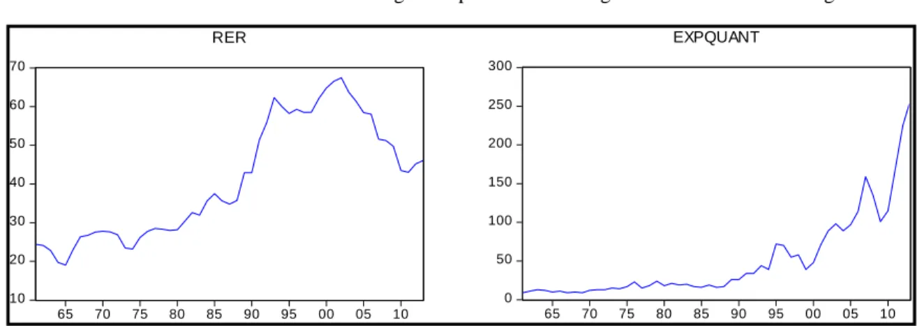
In order to understand the role of exchange rate movements in the dynamics of agricultural exports/imports, we should take a closer look at Figure 1, which shows monthly movements of the quantity of Indian agricultural exports from 1961 through August 2013 using time series provided by the FAOSTAT, where RER and EXPQUANT are the real exchange rate of US dollar and the index of agricultural export quantity of India. As is apparent from the figure that shows the degree of co-movement, as measured by turning points common to the exchange rate of dollar and agricultural export quantity index, if there is depreciation in Indian Ruppee, dollar price will rise and this will eventually lead to an increase in export quantity. Ghosh (1999, 2008, 2013) literature has also studied the structural changes and growth in India and reported that his estimates show significant structural breaks in Indian agriculture in 1967–1968 and 1988–1989 and concluded that best growth performance in agriculture sector was during 1980s.
Figure 1. Real exchange rate and agricultural export quantity index
Agricultural export has been the backbone of India’s export efforts because contributes about 12.3 percent of Gross Domestic Product (GDP) and provides employment to about 58 percent of total population. Moreover, India is also among the world's largest producers and consumers of a range of crop and livestock commodities, and ranked 17th as an agricultural importer and 13th as an exporter during 2011-13 (Landes, 2016). The share of exports in GDP increased from 24 percent in 2012–13 to 24.8 percent in 2013–14, while the share of imports declined from 30.7 percent to 28.4 percent, resulting in improvement in net exports by 3.1 percent points of the GDP (KPMG, 2014). Finally, exchange rate reforms initiated in 1991 has contributed to the significant increases in exports of tradable agriculture and foreign exchange reserve positions.
3. Econometric Methodology
Granger (1969) defines causality between two stationary series x and y in terms of predictability. Let yt and xt represent two stationary and ergodic time series processes. We are interested in exploring whether there is a Granger-causal relationship between the two series without restricting the analysis to a specific functional form. For the null hypothesis variable xt cannot Granger cause yt (Granger, 1988).
1 1 m n t i t i j t j t i j
Y
Y
X
(1)
10 20 30 40 50 60 70 65 70 75 80 85 90 95 00 05 10 RER 0 50 100 150 200 250 300 65 70 75 80 85 90 95 00 05 10 EXPQUANTwhere
Y
t and
X
t are the first difference ofY
t andX
t, respectively,
is a constant, m and n are the lag lengths enough to make disturbance term
t white noise, and t is time.The first step in this analysis concerns the stationary of the series. Since the Granger (1969) approach requires the variables in the system to be stationary, the first step should be to determine whether or not the variables contain unit root. We apply the augmented Dickey–Fuller (ADF) test in our study and select the lag order by the Akaike Information Criterion and Schwarz Information Criterion. Furthermore, if two series are not cointegrated, then we can conclude that a long-term economic relationship exists between them and they move together in the long run. As a result, we should employ the causality test based on a VAR specification rather than a VECM.
On the other hand, one of the most prominent of the nonlinear causality tests is the modified version of the Baek and Brock (1992) test which was developed by Hiemstra and Jones (1994) who allow for the existence of short-term autocorrelations in time series and lately modified by Diks and Panchenko (2006). While the DP test has the ability to detect nonlinear causal relationships, it does not provide any information on the source of nonlinear dependence.
4. Data and Empirical Results
We examine empirically investigate the causal link between the real exchange rate and agricultural exports in India employing a linear and nonlinear causality analysis. We carry out our investigation using annual agricultural export quantity in India and the real Indian Rupee-US Dollar exchange rate data time series data from 1961 to 2013. The data required was collected from Food and Agriculture Organization of the United Nations (FAOSTAT) and Reserve Bank of India. Fig.2 shows the illustrations of evolutions of exchange rate and the quantity of agricultural export in India. Note that there appears to be strong co-movement between exports and exchange rate. However, whether this co-movement relates to causation will be examined using the relevant tests.
Prior to investigating Granger causality, Table 1, the results of unit root tests based on Dickey and Fuller (1979) (ADF) and Phillips and Perron (1988) (PP) reports that the statistics significantly confirm that the level values of both series are non-stationary; that is, both variables are I(1).
Table 1. Unit Root Test
RER EXQ ΔRER ΔEXQ
Intercept only
ADF -1.250522 5.012114 -5.055101*** -5.036708***
PP -1.178347 10.72695 -5.024168*** -4.467875***
Trend and intercept
ADF -0.472924 3.511758 -5.088958*** -5.722048***
PP -1.029917 7.395187 -5.088958*** -5.442542***
Note: The optimal lag lengths are chosen based on Schwarz information criterion (SIC). * rejection of the null hypothesis at 10% significance level.
**rejection of the null hypothesis at 5% significance level. *** rejection of the null hypothesis at 1% significance level.
The next step is to test whether a long-run relationship exists between the variables. As Engle and Granger (1987) states that, since our series are co-integrated, the causality test needs to be applied on a vector error correction model (VECM) rather than an unrestricted vector autoregressive model (VAR). Therefore, we should keep in mind that, before examining causality relationship, we should first check the cointegration relationship between the series. Thus, the Johansen test of cointegration has been conducted to test the long-run cointegrating relation of agricultural export with exchange rate with appropriate assumptions on trends and lags. Table 2 shows that exchange rate is not cointegrated with agricultural export; that is, there is no long-run relationship between exchange rate and agricultural export.
Table 2. Johansen Cointegratin Test
Null Hypothesis Trace Statistics Max-eigen statistic
None 5.932999 5.924840
At most 1 0.008159 0.008159
Based on the first differences of the two series, it can be seen from the Table 3 that the results are not supportive of a Granger-causal relationship between real exchange rate and agricultural export quantity. That is, unidirectional/bidirectional causality relationship does not exist between real exchange rate and agricultural export in India. Table 3 also reports that linear causality behavior between agricultural export and exchange rate does not exist after the procedure of VAR filtering.
Table 3. Results of Linear Causality Analysis
Null Hypothesis F-Statistic 5% Critical Value
RER→EXQ
(Raw Data) 0.046065 0.9772
EXQ→RER
(Raw Data) 3.228999 0.1990
RER→EXQ
(VAR filtered series) 0.029085 0.9856
EXQ→RER
(VAR filtered series) 3.279189 0.1941
Note: Potential heteroscedasticity of the error term is corrected by using White robust standard errors. The lag length selection is based on Schwarz Information Criterion (SIC).
To confirm nonlinear linkages between the series, firstly we employ a BDS test and show the results in Table 4. The BDS approach essentially tests for deviations from identically and independently distributed (i.i.d.) behavior in time series. We choose the lags Ix=Iy=1, the constant C for the bandwidth is set at 1.5 and let the embedding dimension (m) vary from 2 to 61. Because the p values are below 0.05, the existence of non-linear dependencies has been confirmed, the residuals being not normally distributed. That is, the agricultural export and exchange rate display significant nonlinear properties.
Table 4. Linearity Test Results
Dimension BDS Statistic Std. Error z-Statistic Prob.
2 0.188709 0.006604 28.57320 0.0000 3 0.316156 0.010588 29.86050 0.0000 RER 4 0.399697 0.012713 31.43927 0.0000 5 0.445839 0.013361 33.36921 0.0000 6 0.463195 0.012992 35.65190 0.0000 2 0.149519 0.014790 10.10920 0.0000 3 0.235235 0.023873 9.853599 0.0000 EXQ 4 0.285552 0.028888 9.884750 0.0000 5 0.324083 0.030608 10.58824 0.0000 6 0.347510 0.030015 11.57773 0.0000
Note: The 10%, 5%, and 1% critical values are 1.645, 1.960, and 2.575, respectively. See Brock et al. (1995)
The study now proceeds with the investigation of the nonlinear causal connection between the series. Following Bekiros and Diks (2008), it is possible to examine the nonlinear structure of the series in two steps; as first step, the DP nonparametric Granger causality test is employed, then, as second step, to detect strict nonlinear causality in nature, the test is reapplied to the filtered VAR residuals. As Hiemstra and Jones (1994) mentioned, after removing linear causality with a VAR model, any causal linkage between the residuals of VAR model can be considered as nonlinear predictive power. Considering the relatively small sample size of our data, we set the value of the bandwidth equal to 1.5, based on the suggestion of Diks and Panchenko (2006) and the results are discussed for one lag (lx=ly=1). Table 4 provides the linearity test results in order to examine whether any remaining causality relationships are strictly nonlinear.
The results, reported in the corresponding panels of Table 5, show that nonlinear causality relationships do not exist between exchange rate and agricultural export. Our results of linear and non-linear causality behaviors do not support the statement that currency shocks are exogenous to the agricultural exports in India. The depreciation or appreciation of Rupee has no strong influence on India’s quantity of agricultural exports. Therefore, we can say that increases in the
1
quantity of agricultural exports in India are mainly caused by economic growth, rather than the fluctuations in the exchange rate of Indian Rupee.
Table 5. Results of Nonlinear Causality Analysis.
Null Hypothesis T-Statistic 5% Critical Value
RER→EXQ
(Raw Data) 1.271 0.10192
EXQ→RER
(Raw Data) 0.366 0.35729
RER→EXQ
(VAR filtered series) 0.217 0.41414
EXQ→RER
(VAR filtered series) 0.331 0.62980
Note: The common lag length is lx=ly=1
5. Conclusion
This paper has examined the Granger causality between the exchange rate (Indian Rupee versus U.S. dollar) and agricultural exports in India. Because of the strong effect of real exchange rate on the agricultural exports, a policy that dampens the real exchange rate can enhance agricultural exports. Since macroeconomic conditions and policies have a great role in the determination of domestic agricultural sector development, exchange rate policies have also important repercussions on international agricultural trade.
The main goal of this work was to investigate about the link between the quantity of the agricultural exports and exchange rate in India during 1961-2010. To give empirical evidence to this hypothesis the time series analysis was performed and co-integration and causality nexus were explored using linear and non linear Granger causality approaches. Although there is no direct link between Granger causality and causation in economic sense, our findings suggest that the real exchange rate and the quantity of agricultural exports are not co-integrated; that is, there is no long run relationship between exchange rates and agricultural exports in India.
The results of both the linear and nonlinear Granger causality analysis suggest to accept the presence of neutrality hypothesis in the Indian markets which means that the real U.S. exchange rate and the agricultural commodities do not cause each other in a strictly linear and nonlinear sense. That is, our investigation does not provide any evidence of bidirectional or unidirectional causality between the agricultural exports to real exchange rate in India. In other words, , the real exchange rate does not have predictive power for agricultural exports. The drop in the predictive power of exchange rate in explaining the increase or decrease in the quantity of agricultural exports in India may be attributed to the productivity and efficiency in the agricultural sector as the economy expands over time.
While it is difficult to quantify the net effects of exchange rate policies on agricultural trade, it is unrealistic to seperate the exchange rate policies and strengthening competitiveness of agriculture exports. It is obvious that one of the most damaging consequences of overvaluation of a country’s currency is the undesirable impact on agricultural trade of that country. From the emirical findings in this article, it can be concluded that although exchange rate variability cannot be blamed for the loss of competitiveness of agricultural sector in India, agricultural exports value can be improved further if the governemnt enhances export competitiveness and encourage farmers with financial incentives to use high- sophisticated technologies.
References
Akram, Q. F. (2009). Commodity prices, interest rates and the dollar. Energy Economics, 31, 838-851. https://doi.org/10.1016/j.eneco.2009.05.016
Baek, E. G., & Brock, A. W. (1992). A General Test for Non-Linear Granger Causality: Bivariate Model. Technical Report, Korean Development Institute and University of Wisconsin-Madison.
Barichello, R., Pearson, S., & Selim, M. (1998). The Impact of the Indonesian Macroeconomic Crisis on Agricultural Profitabilites. Paper Prepared for USAID Mission, Jakarta, Indonesia.
Bekiros, S. D., & Diks, C. G. H. (2008). The nonlinear dynamic relationship of exchange rates: Parametric and
nonparametric causality testing. Journal of Macroeconomics, 30, 1641-1650.
https://doi.org/10.1016/j.jmacro.2008.04.001
Brock, W., Dechert, W. D., Lebaron, B., & Scheinkman, J. (1995). A Test for Independence Based on the Correlation Dimension, Working papers, Wisconsin Madison - Social Systems.
Dickey, D., & Fuller, W. (1979). Distribution of the Estimato rs for Autoregressive Time Series with a Unit Root. Journal of the American Statistical Association,74, 427-431.
Diks, C., & Panchenko, V. (2006). A new statistic and practical guidelines for nonparametric Granger causality testing.
Journal of Economic Dynamics and Control, 30, 1647-1669. https://doi.org/10.1016/j.jedc.2005.08.008
Engle, R. F., & Granger, C. W. J. (1987). Cointegration and Error Correction: Representation, Estimation and Testing.
Econometrica,55, 251-276. https://doi.org/10.2307/1913236
Frank, J., & Garcia, P. (2010). How strong are the linkages among agricultural, oil, and exchange rate markets?.
Proceedings of the NCCC-134 Conference on Applied Commodity Price Analysis, Forecasting, and Market Risk Management, St. Louis, US.
Ghosh, M. (1999). Structural Break and Unit Root in Macroeconomic Time Series: Evidence from a Developing Economy. Sankhya (The Indian Journal of Statistics), 61, Part 2, Series B, 318-336.
Ghosh, M. (2008). Economic Reforms and Indian Economic Development – Selected Essays, Bookwell, New Delhi. Ghosh, M. (2013). Structural Breaks and Performance in Agriculture. In: Liberalization, Growth and Regional
Disparities in India. India Studies in Business and Economics. Springer, India.
https://doi.org/10.1007/978-81-322-0981-2_6
Granger, C. (1969). Investigating Causal Relations by Econometric Models and Cross-spectral Methods. Econometrica, 37(3), 424-438. https://doi.org/10.2307/1912791
Granger, C. (1988). Some Recent Developments in A Concept of Causality. Journal of Econometrics, 39, 199-211. https://doi.org/10.1016/0304-4076(88)90045-0
Hiemstra, C., & Jones, J. D. (1994). Testing for linear and nonlinear Granger causality in the stock price-volume relation. Journal of Finance, 49, 1639-1664.
Indian Economic Survey 2013-14-Key Highlights, KPMG in India. (July, 2014). Retrieved from www.kpmg.com/in Kapombe, C. M., & Colyer, D. (1999). A Structural Time Series Analysis of U.S. Broiler Exports. American Journal of
Agricultural Economics, 21, 295-307. https://doi.org/10.1016/S0169-5150(99)00030-4
Landes, M. (2016). USDA’s Economic Research Service. Retrieved from
http://www.ers.usda.gov/topics/international-markets-trade/countries-regions/india.aspx
Mathew, S., Terry, R., & Agapi, S. (2006). Exchange rates, foreign income, and US agriculture. Bulletin Number 06-1, Economic Development Center, Department of Applied Economics, University of Minnesota, Minneapolis. Oyejide, T. A. (1986). The Effects of Trade and Exchange rate Policies on Agriculture in Nigeria. IFPRI Research
Report, 55.
Phillip, P., & Perron, P. (1988). Testing for a Unit Root in Time Series Regression. Biometrika, 75(2), 335-346. https://doi.org/10.1093/biomet/75.2.335
Schuh, G. E. (1974). The exchange rate and US agriculture. American Journal of Agricultural Economics, 56(1), 1-13. https://doi.org/10.2307/1239342
Susanti, Y. F. (2001). The effect of exchange rate on Indonesian agricultural exports. PhD dissertation, Oklahoma State University, Stillwater, OK.
Copyrights
Copyright for this article is retained by the author(s), with first publication rights granted to the journal.
This is an open-access article distributed under the terms and conditions of the Creative Commons Attribution license which permits unrestricted use, distribution, and reproduction in any medium, provided the original work is properly cited.