USING GOAL PROGRAMMING TO INCREASE THE EFFICIENCY OF MARKETING CAMPAIGNS

Business Research

1-1-2015

USING GOAL PROGRAMMING TO

INCREASE THE EFFICIENCY OF

MARKETING CAMPAIGNS

Arben Asllani

University of Tennessee at Chattanooga, [email protected]

Alireza Lari

Wake Forest University, [email protected]

Follow this and additional works at:

http://scholars.fhsu.edu/jiibr

This Article is brought to you for free and open access by FHSU Scholars Repository. It has been accepted for inclusion in Journal of International &

Recommended Citation

Asllani, Arben and Lari, Alireza (2015) "USING GOAL PROGRAMMING TO INCREASE THE EFFICIENCY OF MARKETING CAMPAIGNS,"Journal of International & Interdisciplinary Business Research: Vol. 2, Article 6.

USING GOAL PROGRAMMING TO INCREASE THE EFFICIENCY OF

MARKETING CAMPAIGNS

Arben Asllani, University of Tennessee at Chattanooga Alireza Lari, Wake Forest University

Organizations allocate a part of their financial resources to optimize their market segmentation strategies, plan marketing campaigns, and improve customer relationships. Throughout this process, they use a vast amount of electronic records generated by online and offline purchases to design effective marketing campaigns and introduce personalized promotions for their customers by employing data analytics. The problem of selecting target customer segments, given various priorities and the budget constraint, can be modeled as a multi-objective optimization problem with flexible goals and different priorities, interdependencies and resources constraints. The main objective of this paper is to demonstrate the use of the goal programming approach to address this challenge.

Keywords: Goal Programming, RFM, CLV, Linear programming, Marketing Campaigns

INTRODUCTION

Due to the scarcity of resources, companies commonly face the problem of prioritizing the marketing activities in which the firm will invest and determining the levels of funding for those activities. Selecting the best set of marketing activities is not easy as there are numerous factors that must be accounted for.

Organizations must select the most viable marketing activities to maximize the outcomes (e.g. improve customer relationships), and minimize any negative results (e.g. high costs). This requires identifying the most cost-beneficial marketing campaigns.

In order to effectively target marketing activities, it is assumed that different groups of customers want different kinds of services and products, and as a result market segmentation techniques and customer segmentation are widely used.

One option in attempting to select the most effective marketing campaign is the RFM (Recency-Frequency-Monetary) approach. “Recency,” as defined by Fader, Hardie, and Lee (2005), is the time of a customer’s most recent purchase, while “frequency” is the number of past purchases. The literature offers varying definitions of “monetary value” (Fader et al., 2005; Blattberg, Malthouse, and Neslin, 2009; Rhee & McIntyre, 2009). These definitions include average spending per transaction (essentially equivalent to M/F), and the total amount spent by a customer on all purchases over a specified time period. The RFM framework allows for more effective marketing campaigns by categorizing customers into homogenous segments that allow for the design of promotion campaigns that are customized for the particular segment at issue. In this approach, values for R, F, and M are assigned to each customer and are then used to categorize customers to help determine the most effective types of promotions for that specific customer. For example, if a given customer segment shows a low value for recency and relatively high values for frequency and monetary, then this group of customers is typically approached with a “we want you back” marketing strategy. If a given customer segment shows a low value for monetary and high values for frequency and recency, then this group of customers is approached with a “cross selling” marketing strategy.

One drawback is that the RFM approach assumes an unlimited marketing budget and complete access to all the organizations’ customers, even those who have low RFM scores; however, these assumptions are not realistic because organizations tend to operate under annual marketing budget constraints. In addition, the importance of the R, F, and M components in the RFM approach might not be the same. For example, a company might be

mostly interested in the R component, making it a priority to bring back those customers who have taken their business to competitors and thereby placing frequency and monetary values as the second and third priorities, respectively. To properly address and account for budget constraints and marketing priorities, managers must gear their promotional spending strategies toward customers who will yield the greatest growth in cash flows and profits within the given constraints.

Kotler and Armstrong (1996) define a profitable customer as “a person, household, or company whose revenues over time exceed, by an acceptable amount, the company costs of attracting, selling, and servicing that customer.” This excess is called customer lifetime value (CLV). CLV is the sum of cumulated cash flows, discounted using the weighted average cost of capital, of a customer over his/her entire lifetime with the company (Kumar, Ramani, & Bohling, 2004). In the context of customer relationship management, CLV becomes important because it is a metric to evaluate marketing decisions (Blattberg & Deighton, 1996). CLV provides a tool for firms to apply different types of marketing instruments toward different customers based upon their expected values, which may result in better return on the firm’s marketing investment.

In marketing campaigns, managers also strive to find a balance between two types of errors: ignoring those customers who could have returned to create more revenue for the organization, and investing on those

customers who are not yet ready to purchase. Venkatesan and Kumar (2004) refer to these errors as Type I and Type II errors. It is therefore important for marketing campaign decision-makers to understand the importance of these two error types and to adjust their decisions accordingly.

In order to create effective marketing campaigns, companies use a vast amount of electronic records generated by online and offline purchases and use data analytics to design effective marketing campaigns and introduce personalized promotions for their customers. As a result, for any effort in determining the most effective campaign strategy, there will be a need for analytical tools that can help the decision makers in choosing the optimal strategy.

This paper presents a goal programming model that balances Type I and Type II errors by identifying the RFM segments that should be reached and the RFM segments that are not worthy of pursuit because they lack profitability, do not follow priorities, or exceed marketing budget constraints. The model can help marketers determine whether to follow or cut back on their relationship with a given customer segment. A novel characteristic of this model is the inclusion of campaign priorities and budget constraints to determine which segment of customers should be deemed the optimal targets of a direct marketing campaign.

LITERATURE SURVEY

This section discusses the use of analytics in marketing, summarizes the existing literature on RFM and CLV and explains how these concepts can be used in the proposed goal programming model.

Managers use vast amounts of electronic records to make better decisions. Many online retailers have developed web-based information systems to collect data and use different analytical tools in order to make sound marketing decisions. Aberdeen Group Inc.'s survey of 458 businesses shows that 120 of these businesses are using customer analytics tools and processes as part of their customer management activities (Minkara, 2012). Analytical tools have been used in several marketing research studies. Hung et al. (2012) present a hybrid multi-criteria decision making (MCDM) model that includes a decision-making trial and evaluation laboratory-based analytics network process for online reputation management, to evaluate performances and improve professional services of marketing. They found that the dimension that professional services of marketing should improve first when carrying out online reputation management is online reputation. Kwak, Schniederjans, and Warkenin (1991), used linear goal programming to determine the optimal distribution structure of a manufacturer of food products. The model helps decision makers determine the optimal

distribution structure in terms of the percentage of all commodity volume. In this model, the goal constraints are market share, profit and budget. To address the decreasing response to direct marketing campaigns, marketers use data mining techniques. Many data-mining applications have been developed to discover useful customer

communicating the right offer to the right customer at the right time. Breur (2007) argues that when both the marketing offer and targeting are tested at the same time, it is not clear whether the higher response to the new campaign can be attributed to an improvement of the marketing offer or to better targeting. He proposes a comprehensive test-design to evaluate the relative contribution of the marketing offer and targeting (data mining models). This provides decision makers with a framework for campaign planning and evaluation. With the increase in using large data sets and analytical tools for better decisions, the trend of introducing new modeling approaches will continue.

In order to identify segments of like-minded customers, the SAS System has introduced different clustering algorithms that provide a range of algorithms for discovering market segments. The cluster analysis, which is an empirical technique, has been used as a tool for information visualization. Pratter (n.a.) has used the Fisher iris data of 1936 from the library of SAS sample programs to show that cluster analysis will always result in a set of segments. He warns the researchers about the face validity of the segments. Bose & Chen (2009) present different methods for customer clustering and pattern recognition.

The concepts of cluster analysis for segmentation have also been discussed by Venkatesan (2007). He defines segmentation as:

“a way of organizing customers into groups with similar traits, product preferences or expectations. Once segments are identified, marketing messages and in many cases even products can be customized for each segment. The better the segments chosen for targeting a particular organization, the more successful it is assumed to be in the marketplace. Segments are constructed on the basis of customers’ a) demographic characteristics, (b) psychographics, c) desired benefits from product/services, and d) past-purchase and product-use behaviors.”

Clustering analysis as a data mining approach was used by Saglam, Salman, Sayin, and Turkay (2006) to identify groups of entities that are similar to each other with respect to certain measures. They proposed a mixed integer programming model based on the clustering approach to a digital platform company’s segmentation problem that includes demographic and transactional attributes related to the customers. The objective function was to minimize the maximum cluster diameter among all clusters with the goal of establishing evenly compact clusters. The authors used a real problem from a satellite broadcasting company with 800,000 customers, to test the performance of the proposed approach and found that it creates meaningful segmentation of data.

Many researchers have addressed the subject of customer preferences measurement. Scholz, Meissner, and Decker (2010) have used a compositional approach based on paired comparisons to measure customer

preferences for complex products. This approach accounts for response errors and thus allows for elicitation of more precise preferences. They benchmark this technique against adaptive conjoint analysis and computer-based self-explication of multi-attribute preferences to show the relative validity and accuracy in two empirical studies. Knowing what the customer wants is still the base for choosing proper strategies for marketing campaigns.

In an effort to select the most effective marketing campaigns, researchers and practitioners have made use of CLV and RFM concepts. CLV is the net present value of cash flows expected over the life of the relationship between the customer and the firm. In the calculation of CLV, Blattberg et al. (2009) suggest to include factors such as the expected length of the customer-firm relationship, the expected marketing costs and expected revenues generated throughout the life of this relationship, and the discount rate. In addition, Blattberg et al. (2009) have identified variables such as customer satisfaction, marketing efforts, cross-buying, and

multichannel purchasing to have a positive impact on CLV. CLV is a metric used to measure the profitability of each customer, and serves as a target metric when designing marketing campaigns (Pfeifer & Carraway, 2000; Venkatesan, Kumar, & Bohling, 2007; Forbes, 2007, Blattberg et al., 2009), as well as a guide for customer relationship management decisions (Zeithaml, Bitner & Gremler, 2009; Haenlein, Kaplan, & Beeser, 2007; Jackson, 2007; Zeithaml, Rust, & Lemon, 2001).

An accurate estimation of CLV may prove to be difficult for many firms (Stahl, Matzler, & Hinterhuber, 2003; Vogel, Evanschitzky, & Ramaseshan, 2008), which indicates a need for a method that would allow for

relatively simple predictions of customers' potential profitability and effective customer relationship management (CRM) decision inputs.

Borle, Sharad, Singh, Siddharth, and Jain (2008) have used a hierarchical Bayes’ approach to estimate the lifetime value of each customer at each purchase occasion by jointly modeling the purchase timing, purchase amount, and risk of defection from the firm for each customer. The results show that longer inter-purchase times are associated with larger purchase amounts and a greater risk of leaving the firm. In order to predict CLV, Ekinci, Ulengin, Uray, & Ulengin (2014) proposed a model that predicts the potential value of the current customers rather than measuring the current value. The Markovian-based model proposed by these authors helps companies with several types of products to make future marketing decisions. The empirical validity of the model was tested in the banking sector.

One of the tools used to categorize customers according to profitability potential for future direct marketing investment is RFM. It is used as a promotional tool that allocates spending based on the amount of customers’ purchases instead of the length of their relationship with the firm (Reinartz & Kumar, 2000). Customers who create high revenues for the organization will receive a higher level of promotional spending (Venkatesan et al., 2007). Recency, frequency and monetary values are not always equally weighted, and recency often has a greater weight as it may be used to signal the end of the customer-firm relationship; a long period of customer inactivity may be indicative of this termination (Dwyer, 1989). Less emphasis is put on monetary value, and the least on frequency (Reinartz & Kumar, 2000; Venkatesan et al., 2007).

Among the many analytical tools used for marketing campaigns, RFM remains popular due to its simplicity of use. Many marketing data mining algorithms, and in particular the ones for direct marketing, are based on this concept (McCarty & Hastak, 2007). The use of such data mining techniques allow marketers to better manage their customers’ databases for segmentation and generate more effective and cost efficient promotional strategies for direct marketing campaigns. Bose & Chen (2009) reviewed research in the area of quantitative models for direct marketing from a system perspective. In this study, they show that two types of models, statistical and machine learning based are popular. They present the advantages and disadvantages of each type of model.

Venkatesan et al., 2007 have reported other methods in addition to RFM analysis for evaluation of

customer selection during a marketing campaign, and estimation of the future value of customers. Some of these methods (e.g. return on equity) evaluate the financial return from particular marketing expenditures such as direct mail and sales promotion (Rust, Lemon, & Zeithaml, 2004). Elsner, Krafft, and Huchzermeier (2003) discuss other applications of RFM that go beyond its “traditional” direct marketing approach and provide a dynamic heuristic model. This model combines a chi-square automatic detection interaction algorithm with recency, frequency, and monetary value segmentation to determine the optimal frequency of catalog mailings for a company in the mail order business. This will help marketers predict the time when customers should receive reactivation packages.

Bhasker et al. (2009) utilized mathematical programming (MP) and RFM analysis for personalized promotions for multiplex customers, incorporated business constraints, and then, provided useful insights, aiding the multiplex in implementing an effective loyalty program. The researchers separated RFM from MP in their algorithm, using RFM is for non-recent customers and MP for current customers.

This paper presents a goal programming model that uses data from an RFM analysis and the annual budget constraints on the marketing campaigns. Incorporating RFM data into a single goal programming model for all potential direct marketing campaign target customers is a major contribution of this research.

THE PROPOSED GOAL PROGRAMMING FORMULATION

The Approach

Goal Programming (GP) is a multi-objective mathematical programming approach with several objectives where some are treated as constraints instead of objectives. In this type of mathematical programming, the model automatically adjusts the level of certain resources to satisfy the goal of the decision maker.

When developing an advertising campaign, the manager needs to decide the cutoff points for recency (R), frequency (F), and monetary (M) values with the goal of maximizing overall customer lifetime value (CLV) within a limited budget. If the modeler is not concerned with F and M, then we would have a simple linear program to determine the cutoff point for R. For this simple linear program, the solution process will generate a maximum CLV based on recency only, which is VR.

Similarly, for Frequency only, not considering M and R, we will have a simple linear program that finds VF as the maximum CLV for the cutoff value of F. In the case of modeling the linear program for M, the maximum CLV for the M cutoff point is VM. The modeler may take each of the values VR, VF, and VM found in solving the corresponding linear programs as a "goal'' and try to find a solution that comes close to all of the goals. Since it may not be possible to reach all of the goals simultaneously, the modeler will create a set of penalties for not reaching a goal. These penalties depend on the importance of reaching a particular segment. For example, if the modeler values R more than F, and then F more than M, the penalties could be P1, P2 and P3 respectively, where P1>P2>P3>0. The modeler will create new variables s1, s2, and s3 to represent the failure of meeting goal 1, 2, and 3 respectively, and creates the following linear program:

Minimize P1s1 + P2s2 + P3s3 Subject to

{Objective function of the R model} + s1 = VR {Objective function of the F model} + s2 = VF {Objective function of the M model} + s3 = VM + any other constraints, including budget constraints

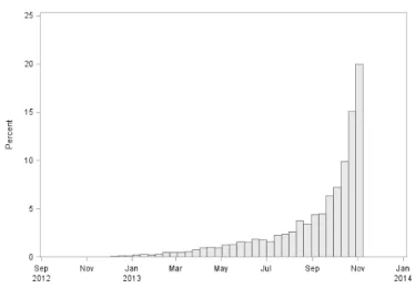
In order to illustrate the proposed GP model, a sample of 543,311 real customer transactions from a chain of brewery-based restaurants is used. These data represents transactions of 23,239 customers who had visited one of the restaurants at least three times. Since frequency is an important variable in the proposed model, the data were filtered to show those customers who have shown “some degree” of loyalty. Each data point in this study contains the customer’s ID, the last transaction date (as recency), number of transactions (as frequency), and the average sales per customer (as monetary value). Summary statistics for number of visits and average sales are shown in Figure 1. The selected customers have visited the stores on average about 12.82 times and every time they have spent an average of $32.81. Figure 2 shows the distribution of the most recent visit. As shown, about 20 percent of the customers still continued to visit the store at the time of data collection.

Figure 1: Summary Statistics for Frequency and Monetary Value

Figure 2: Histogram for Most Recent Visit

THE OPTIMIZATION MODELS’ NOTATIONS

i= index for the group of customers in a given recency category (i=1,…,5); j= index for the group of customers in a given frequency category (j=1,…,5); k= index for the group of customers in a given monetary category (k=1,…,5); V= Expected revenue from a returned customer;

pi= the probability for a group i recency customer to make a purchases; pj= the probability for a group j frequency customer to make a purchase; pk= the probability for a group k monetary customer to make a purchase; Ni= number of current customers in recency group i;

Nj= number of current customers in frequency group j; Nk= number of current customers in monetary group k;

C= average cost of reaching a customer during the marketing campaign; B= budget ceiling for the marketing campaign;

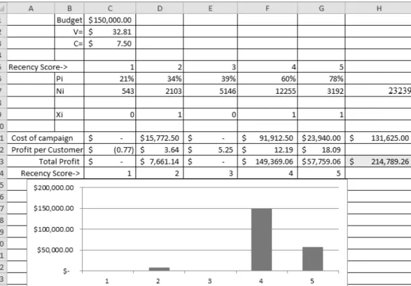
Indices i, j, and k and their respective categories are defined on consultation with company management. The cut-off points for each category are shown in Figure 3 and are based on previous experience with similar groups of customers, business dynamics, and sales data. The goal of the company is to decide whether to reach or not reach customers in a certain category considering a limited marketing budget of $150,000 per campaign. Three separate LP models, one for each category, are formulated and solved. Then, each of these solutions is incorporated into the last goal programming model which aims to identify best customer categories to achieve several priority goals.

Figure 3: Cut-off Points for Each Category

ƵƚͲŽĨĨWŽŝŶƚƐ ĨŽƌZĞĐĞŶĐLJ ŝͲŝŶĚĞdž ƵƐƚŽŵĞƌƐŝŶ ĂƚĞŐŽƌLJ ƵƚͲŽĨĨWŽŝŶƚƐ ĨŽƌ&ƌĞƋƵĞŶĐLJ ũͲŝŶĚĞdž ƵƐƚŽŵĞƌƐŝŶ ĂƚĞŐŽƌLJ ƵƚͲŽĨĨWŽŝŶƚƐĨŽƌ DŽŶĞƚĂƌLJsĂůƵĞ ŬͲŝŶĚĞdž ƵƐƚŽŵĞƌƐŝŶ ĂƚĞŐŽƌLJ Ϭ ϭ ϱϰϯ Ϭ ϭ ϱ͕ϭϰϵ ΨϬ͘ϬϬ ϭ ϱ͕ϴϱϱ ϯͬϭͬϮϬϭϯ Ϯ Ϯ͕ϭϬϯ ϱ Ϯ ϵ͕ϴϬϬ ΨϮϬ͘ϬϬ Ϯ ϱ͕ϴϵϮ ϲͬϭͬϮϬϭϯ ϯ ϱ͕ϭϰϲ ϭϬ ϯ ϯ͕ϮϯϮ ΨϯϬ͘ϬϬ ϯ ϱ͕Ϭϴϯ ϵͬϭͬϮϬϭϯ ϰ ϭϮ͕Ϯϱϱ ϭϱ ϰ ϭ͕ϲϭϯ ΨϰϬ͘ϬϬ ϰ ϯ͕ϯϭϵ ϭϭͬϭͬϮϬϭϯ ϱ ϯ͕ϭϵϮ ϮϬ ϱ ϯ͕ϰϰϱ ΨϱϬ͘ϬϬ ϱ ϯ͕ϬϵϬ dŽƚĂů Ϯϯ͕Ϯϯϵ dŽƚĂů Ϯϯ͕Ϯϯϵ dŽƚĂů Ϯϯ͕Ϯϯϵ

FORMULATION AND SOLUTION PROCESS OF INTEGER LINEAR PROGRAMMING MODEL FOR THE RECENCY CASE

The objective for this 0-1 LP model with recency dimension is to maximize the profits from potential customer purchases within the given budget.

Consider the decision variable as:

xi = 1 if the marketing campaign reaches customers in recency i; 0, otherwise

The mixed 0-1 integer linear programming formulation is: Objective Function: Maximize:

¦

−

=

N

p

V

C

x

Z

)

(

B

Cx

N

≤

¦

{ }

0

,

1

=

x

The objective function maximizes the expected profit (Zr) of the marketing campaign. A customer in a state of recency “i” has a pi chance of purchasing (with a profit of “V-C”) and a (1- pi) chance of not purchasing (with the expected profit of”– C”). Therefore, the expected value of the profit from a single customer in state i is:

)

)(

1

(

)

(

V

C

p

C

p

−

+

−

−

C

V

p

−

, (5)

For the Ni customers in recency i, the expected profit from this group of customers is:

)

(

p

V

C

N

−

, (6)

In the above formulation, equation (1) indicates the sum of profits for all the groups of customers who are targeted for advertisement (xi=1) and equation (2) imposes the budget limitations (B) for this marketing campaign. The left side of the equation that shows the sum of campaign costs for each group “i” of customers represents the actual cost of the campaign.

In order to solve the above problem, the following steps are followed:

1. The customers are divided into groups 1 through 5 where group 1 represents the customers with the least recent purchases and group 5 represents the ones with the most recent transactions.

2. The number of customers in each group is calculated by using a pivot table that shows nip, the number of customers in recency i who make a purchase within the next month. The probability that a customer in group i will purchase is calculated as:

i ip i

N

n

p

=

As indicated in Figure 4, given a campaign budget of B= $150,000, a cost of C= $7.50 to reach a customer, and the average revenue of V=$32.81 from the purchasing customer, the company should only select customers of recency 2, 4, and 5 for future promotional efforts. Customers who belong to recency 2 can simply be ignored due to the small contribution in the overall profit as shown

graphically. This solution will generate a total profit of $214,789.

Figure 4: LP Formulation and Solution for the Recency Case

FORMULATION AND SOLUTION PROCESS OF INTEGER LINEAR PROGRAMMING MODEL FOR THE FREQUENCY CASE

The objective for this 0-1 LP model with frequency dimension is to maximize the profits from potential customer purchases within the given budget.

The decision variable for this case is a 0-1 variable with the following definition: Xj = 1 if the marketing campaign reaches customers in frequency j; 0, otherwise;

Objective Function: Maximize:

¦

−

=

N

p

jV

C

x

Z

)

(

B

Cx

N

≤

¦

{ }

0

,

1

=

x

The objective function in equation (8) maximizes the expected profit (Zf) of the marketing campaign. There is a chance of pj for a customer in a state of frequency j to purchase and a chance of (1- pj) not to purchase. The profit from a customer is calculated as (jV-C) when there is a purchase, otherwise the expected profit is (-C). Therefore, the expected profit from a single customer in state “j” is:

)

)(

1

(

)

(

jV

C

p

C

p

−

+

−

−

C

jV

p

−

For Nj customers with frequency j, the expected profit of this group of customers is:

)

(

p

jV

C

N

−

With this explanation, equation (8) shows the total profit for groups of customers for which the marketing decision to reach them is made. The left side of equation (9) represents the actual cost of the campaign, which is calculated as the sum of campaign costs for each group i of customers and should not exceed the budget ceiling of “B.”

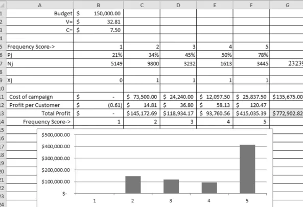
There are companies that consider recency and frequency as the only two significant values in their direct marketing campaign. In this situation, customers are first organized into groups (in this case 5 groups), with each Gj group containing customers from frequency value j (1, 2…, 5). Again, companies are interested in determining the customer groups that should be targeted and reached. Similar to the previous case, the number of customers in each group is calculated using a pivot table. If the number of customers in group Gj is considered to be Nj, then the probability that a customer in this group will purchase is calculated as:

j jp j

N

n

p

=

Figure 5: LP Formulation and Solution for the Frequency Case

The results of the frequency solution are shown in Figure 5. The solution indicates that customers in the frequency 2, 3, 4, and 5 must be reached. This solution will generate a total profit of $772,902.

FORMULATION AND SOLUTION PROCESS OF INTEGER LINEAR PROGRAMMING MODEL FOR THE MONETARY CASE

The LP model of this section includes monetary value. The objective function is to maximize the profit from potential customer purchases within the budget limits.

The decision variable is defined as:

xk = 1 if the marketing campaign reaches the customers in monetary group k 0, otherwise; Objective Function Maximize:

¦

−

=

N

p

kV

C

x

Z

)

(

B

Cx

N

≤

¦

{ }

0

,

1

=

x

The objective function in equation (15) maximizes the expected profit (Zm) of the marketing campaign. There is a pk chance for a customer in a state monetary k of purchasing and a (1- pk) chance of not purchasing. When purchasing, the profit from a customer is calculated as (V-C). When not purchasing, the expected profit is simply (-C). The expected value of the profit from a single customer in state k is:

)

)(

1

(

)

(

kV

C

p

C

p

−

+

−

−

C

V

p

−

With Nk customers with monetary k, the expected profit is:

)

(

p

kV

C

N

−

Equation (16) creates a budget limit of B for this marketing campaign.

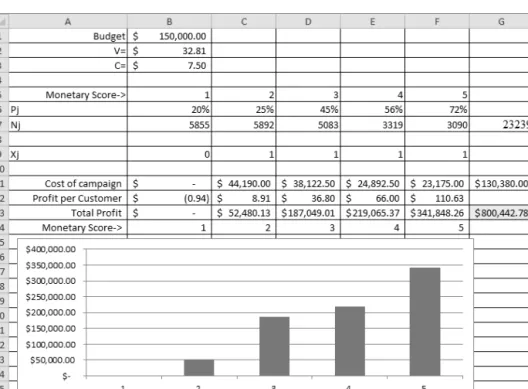
An optimal solution summary for the monetary model is presented in Figure 6. This figure indicates the segments that are profitable for the company. The future promotional campaign must include customers with monetary values of 2, 3, 4, and 5 as these segments are clearly profitable. This solution will generate a total profit of $800,442.

GOAL PROGRAMMING MODEL: INCORPORATING PRIORITIES

The comparison of the maximum profit from each of the above three models indicates that monetary value score is the most important variable of the RFM framework. The next important variable is frequency, followed by recency. However, the marketing department is interested in investigating the impact of setting the

following priorities:

• Priority 1 (P1 = 3): Recency • Priority 2 (P2 = 2): Frequency • Priority 3 (P3 = 1): Monetary

The following is the LP formulation, which minimizes the penalties of not reaching the goals:

Minimize 3s1 + 2s2 + 1s3 (21) Subject to:

¦

−

p

V

C

x

N

)

(

¦

−

p

jV

C

x

N

)

(

¦

−

p

kV

C

x

N

)

(

B

Cx

N

Cx

N

Cx

N

+

¦

+

¦

≤

¦

{ }

0

,

1

=

x

{ }

0

,

1

=

x

{ }

0

,

1

=

x

In the above formulation, (21) represents the objective function. Minimization of s1 has priority over minimization of s2, since s1 has a larger contribution coefficient (3>2). Similarly, minimizing s3 has the lowest priority. Equations (22), (23), and (24) represent the new set of constraints added to the model to make sure that profit goals VR= $214,789, VF= $772,902, and VM= $800,442 are set to be achieved. Equation (25) assures that the overall budget (B=150,000) is not exceeded. Finally, equations (26), (27), and (28) ensure binary solution values for the decision variables.

SOLVING THE OVERALL MODE

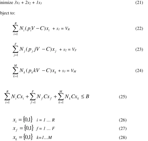
Figure 7 shows the optimal solution to the goal programming approach. As seen, the total profit for the solution is $1,254,064 and the solution suggests that the manager must reach customers with a recency score of

Figure 7: Optimal solution for the GP model

CONCLUSIONS AND RECOMMENDATIONS

The analysis presented here provides the optimal solutions for different variations of the RFM model: a recency model, a frequency model, a monetary value model, and a full RFM-goal programming model with priority constraints. Table 1 compares the final solutions for each model. Because of set priorities, the optimal solution for the GP model is different from the solutions suggested by each individual LP model. For example, while the recency LP model suggests reaching customers with a score of 2, 4, and 5, the GP model suggests that only customers with a recency score of 2 and 5 must be reached. Dropping the segment with recency score 4 seems contradictory to the high priority given to recency. However, while the LP model only considers recency, GP model considers all three factors, although recency has the highest priority. When moving from frequency LP model to GP model, the customers with a frequency score of 2 are dropped from the marketing campaign. Similarly, due to the lowest priority given, the monetary value score of 2 and 3 are not considered in a marketing campaign with set priorities.

This solution is constrained by the campaign budget of $150,000 and generates a total profit of $1,254,064.

Table 1: Summary of Results of Different Approaches

Organizations have limited marketing resources and managers are forced to prioritize their promotional spending. Given the traditionally small response rates in many direct marketing campaigns (e.g., 1.65% for direct mail prospect lists to 4.41% for outbound telemarketing house lists), spending scarce resources to reach

customers who are not ready to purchase (a Type II error) may not be the best strategy (Farrante, 2009; Venkatesan & Kumar, 2004). Use of analytics can help managers better manage their scarce resources and establish a balance between Type I (missing customers who are potentially profitable) and Type II errors by identifying RFM segments that should be reached and RFM segments that are not worthy of pursuing because they are unprofitable or may lead to exceeding budget constraints.

By identifying the most profitable customer segments (given certain marketing costs to reach a customer and total marketing budget constraints), a goal programming approach applied to RFM data can, in a single model, provide direct marketing companies with the capabilities of making optimum decisions regarding future promotional investments. Depending on a customer segment’s profit maximization potential, a direct marketing firm can determine whether to continue its promotional spending in an attempt to generate future sales, or whether it should curtail spending and allocate those marketing resources to other, more profitable customer targets.

This paper can be used as a template for practitioners to utilize and transform purchasing history data into a decision model. The specific contribution of this paper is on considering budget constraints and assigning priorities to customer segments which are based on RFM.

The study has several limitations, all of which provide avenues for ongoing research. First, some have raised the issue of whether RFM can accurately predict future behavior or profitability, given that RFM frameworks represent past or historical behavior (Blattberg et al., 2009; Rhee & McIntyre, 2009). Of course, uncertainty in predicting behavior is inherent in any consumer decision model, and this example is no

exception. Accuracy in prediction will always be a potential limitation when forecasting is based on historical data. In addition, the current model is limited to a six-month time frame, whereas Venkatesan et al. (2007) note that three years is generally considered a good horizon for estimates of CLV and for CRM decisions such as customer selection. While this research does not estimate CLV, future applications might go beyond six months. The static nature of this model could be perceived as a potential limitation, although it does have the advantage of simplicity and ease of use for most organizations (as compared to CLV calculations).

This study made no assumptions about the nature of the costs used in the RFM model. Ultimately, assumptions regarding costs have an impact on CLV, and therefore may impact any RFM model as well. For example, if only variable costs of serving a customer are considered (i.e., marginal costing) as compared to full costs (with overhead allocation), the calculation of CLV could be quite different. Blattberg, Kim, and Neslin (2008) argue for marginal costing since full costing raises costs and can lead to the rejection of some customers (customers who would increase profits if they were targeted). Blattberg et al. (2009) also support the argument for marginal costing, but note that both full costing and marginal costing applications have been found in the literature. Again, these cost issues relate primarily to the prediction of CLV rather than to RFM analysis; but they do suggest that careful determination of costs is necessary. Future RFM research should take these potential limitations into account in order to continually improve the utility and reliability of this analytical method.

WORKS CITED

Bhaskar, T., Subramanian, G., Bal, D., Moorthy, A., Saha, A., & Rajagopalan, S. (2009).An Optimization Model for Personalized Promotions in Multiplexes. Journal of Promotion Management, 15(1/2), 229-246.

Blattberg, R.C., & Deighton, J. (1996, July-August). Manage marketing by the customer equity test, Harvard Business Review, 136-144.

Blattberg, R.C., Malthouse, E.C., & Neslin, S.A. (2009).Customer Lifetime Value: Empirical Generalizations and Some Conceptual Questions. Journal of Interactive Marketing, 23(2), 157-168.

Borle, Sharad, Singh, Siddharth S., & Jain D. C. (2008, January). Customer lifetime value measurement, Management Science, 54(1), 100-112

Bose, I., & Chen X. (2009). Quantitative models for direct marketing: a review from systems perspective. European Journal of Operational Research, 195, 1 – 16.

Breur, Tom. (2007). How to evaluate campaign response – The relative contribution of data mining models and marketing execution. Journal of Targeting, Measurement and analysis for Marketing, 15, pp 103-112, doi: 10.1057/palgrave.jt.5750036

Dwyer, R. F. (1989).Customer Lifetime Valuation to Support Marketing Decision Making. Journal of Direct Marketing, 3(11), 6-13.

Ekinci, Y., Ulengin, F., Uray, N., & Ulengin, B. (2014). Analysis of customer lifetime value and marketing expenditure decisions through a Markovian-based model, European Journal of Operational Research,

http://dx.doi.org/10.1016/j.ejor.2014.01.014

Elsner, R., Krafft, M., & Huchzermeier, A. (2003). Optimizing Rhenania's Mail-Order Business through Dynamic Multilevel Modeling. (DMLM). Interfaces, 33(1), 50-66.

Fader, P. S., Hardie, B. G. S., & Lee, K. L. (2005).Counting Your Customers the Easy Way: An Alternative to the Pareto/NBD Model. Marketing Science, 24(Spring), 275–284.

Ferrante, A. (2009). New DMA Response Rate Study Shows Email Still Strong for Conversion Rates. DemandGen Report, The Scorecard for Sales & Marketing Automation. Retrieved March 16, 2010, from http://www.demandgenreport.com/home/arcives/feature-articles/183-new-dma-response-rate-study-shows-email-still-strong-for-conversion-rates

Forbes, T. (2007).Valuing Customers. Journal of Database Marketing & Customer Strategy Management, 15(1), 4-10.

Haenlein, M., Kaplan, A., & Beeser, A. (2007). A model to determine customer lifetime value in a retail banking context. European Management Journal, 25(3), 221 – 234.

Hung, Y.H., Huang, T. L., Hsieh, J.C., Tsuei, H.J., Cheng, C.C., & Tzeng, G.H. (2012-November). Online reputation management for improving marketing by using a hybrid MCDM model. Knowledge-based Systems, 35, 87-93.

Jackson, T. W. (2007). Personalisation and CRM. Journal of Database Marketing & Customer Strategy Management, 15(1), 24-36.

Kotler, P., & Armstrong, G. (1996). Principles of Marketing, 7th _{edition. Englewood cliffs, N.J.: Prentice-Hall.}

Kumar, V., Ramani, G., & Bohling, T. (2004). Customer Lifetime Value Approaches and Best Practice Applications. Journal of Interactive Marketing, 18(3), 60-72.

Kwak, N.K., Schniederjans, M.J., & Warkentin, K.S. (1991). An application of linear goal programming to the marketing distribution decision. European Journal of Operational Research, 52(3), 334-344.

Lin, Q. Y., Chen, Y.L., Chen, J.S., & Chen Y. C. (2003). Mining inter-organizational retailing knowledge for an alliance formed by competitive firms, Information and Management, 40(5), 431 – 442.

McCarty, J. A., & Hastak, M. (2007). Segmentation Approaches in Data-mining: A Comparison of RFM, CHAID, and Logistic Regression. Journal of Business Research, 60(6), 656-662.

Minkara, O. (2012, Winter). The Middle Ground. Marketing Research, 24(4), 22-29.

Pfeifer, P. E., & Carraway, R.L. (2000). Modeling Customer Relationships as Markov Chains. Journal of Interactive Marketing, 14(2), 43-55.

Pratter, F. (n.a.). Clustering for market segmentation, Retrieved on February 14, 2014, from

http://www.nesug.org/Proceedings/nesug97/infviz/pratter.pdf

Reinartz, W. J., & Kumar, V. (2000). On the Profitability of Long-Life Customers in a Noncontractual Setting: An Empirical Investigation and Implications for Marketing. Journal of Marketing, 64(October), 17-35. Rhee, E., & McIntyre, S. (2009). How Current Targeting Can Hinder Targeting in the Future and What To Do

About It. Journal of Database Marketing & Customer Strategy Management, 16(1), 15-28.

Rust, R. T., Lemon, K. N., & Zeithaml, V. A. (2004). Return on Marketing: Using Customer Equity to Focus Marketing Strategy. Journal of Marketing, 68(January), 109 – 127.

Saglam, B., Salman, F.S., Sayin, S., & Turkay, M. (2006). A mixed integer programming approach to the clustering problem with an application in customer segmentation. European Journal of Operational Research, 173, 866 - 879.

Scholz, S., Meissner, M., & Decker, R. (2010, August). Measuring consumer preferences for complex products: a compositional approach based on paired comparisons, Journal of Marketing Research, 47(4), 685-698.

Stahl, H. K., Matzler, K., & Hinterhuber, H. H. (2003).Linking Customer Lifetime Value with Shareholder Value. Industrial Marketing Management, 32(4), 267 - 79.

Venkatesan, R. (2007). Cluster analysis for segmentation, (publication number UVA-M-0748). Retrieved on February 14, 2014 from http://faculty.darden.virginia.edu/GBUS8630/doc/M-0748.pdf

Venkatesan, R., & Kumar, V. (2004).A Customer Lifetime Value Framework for Customer Selection and Resource Allocation Strategy. Journal of Marketing, 68(October), 106–25.

Venkatesan, R., Kumar, V., & Bohling, T. (2007).Optimal Customer Relationship Management Using Bayesian Decision Theory: An Application for Customer Selection. Journal of Marketing Research,

44(November), 579–594.

Vogel, V., Evanschitzky, H., & Ramaseshan, B. (2008).Customer Equity Drivers and Future Sales. Journal of Marketing,72 (November), 98-108.

Zeithaml, V. A., Bitner, M. J., & Gremler, D.D. (2009). Services Marketing: Integrating Customer Focus across the Firm. New York: McGraw-Hill Publications.