Regional Research Institute Publications and
Working Papers
Regional Research Institute
5-13-2013
A J-test for Panel Models with Fixed Effects, Spatial
and Time
Harry H. Kelejian
Gianfranco Piras
Follow this and additional works at:
https://researchrepository.wvu.edu/rri_pubs
Part of the
Regional Economics Commons
This Working Paper is brought to you for free and open access by the Regional Research Institute at The Research Repository @ WVU. It has been accepted for inclusion in Regional Research Institute Publications and Working Papers by an authorized administrator of The Research Repository @ WVU. For more information, please [email protected].
Digital Commons Citation
Kelejian, Harry H. and Piras, Gianfranco, "A J-test for Panel Models with Fixed Effects, Spatial and Time" (2013).Regional Research Institute Publications and Working Papers. 11.
Regional Research Institute
Working Paper Series
A
J
-test for Panel Models with Fixed Effects, Spatial and Time
Dependence
By: Harry H. Kelejian, Professor of Economics, University of Maryland and Gianfranco Piras, Research Assistant Professor, West Virginia University
Working Paper Number 2013-03
Website address:
rri.wvu.edu
Regional Research Institute
Working Paper Series
A
J
-test for Panel Models with Fixed Effects, Spatial and Time
Dependence
By: Harry H. Kelejian, Professor of Economics, University of Maryland and Gianfranco Piras, Research Assistant Professor, West Virginia University
Working Paper Number 2013-01
Website address:
rri.wvu.edu
A
J
-test for panel models with fixed effects, spatial and time
dependence
∗Harry H. Kelejian University of Maryland College Park, MD 20742, USA
Gianfranco Piras† West Virginia University Morgantown, WV 26506, USA May 13, 2013
∗
We would like to thank the referees and the editor Hashem Pesaran for helpful comments on an earlier version of this paper. They are not, however, responsible for any shortcoming remaining in this paper.
†
Piras is the contacting author: Regional Research Institute, West Virginia University, 886 Chestnut Ridge Road, Room 510, P.O. Box 6825, Morgantown, WV 26506-6825; E-mail: [email protected]; Tel: 304-293-2643; Fax: 304-293-6699.
Abstract
In this paper we suggest aJ-test in a spatial panel framework of a null model against one or more alternatives. The null model we consider has fixed effects, along with spatial and time dependence. The alternatives can have either fixed or random effects. We implement our procedure to test the specifications of a demand for cigarette model. We find that the most appropriate specification is one that contains the average price of cigarettes in neighboring states, as well as the spatial lag of the dependent variable. Along with formal large sample results, we also give small sample Monte Carlo results. Our large sample results are based on the assumption N → ∞and T is fixed. Our Monte Carlo results suggest that our proposed J-test has good power, and proper size even for small to moderately sized samples.
JEL classification: C01, C12
Key Words: Spatial Panel Models, Fixed Effects, Time and Spatial Lags, Non-nested J-test
1
Introduction
The J-test is a procedure for testing a null model against non-nested alternatives.1 As de-scribed in Kelejian and Piras (2011), the J-test is based on whether or not predictions of the dependent variable based on the alternative models add significantly to the explanatory power of the null model.
Kelejian (2008) extended the J-test procedure to a spatial framework, but the suggested test was not based on all of the available information. This was pointed out by Kelejian and Piras (2011) who, among other things, generalized Kelejian’s assumptions. However, neither Kelejian (2008) nor Kelejian and Piras (2011) considered a panel data framework. This is unfortunate because a great many studies in recent years have been in a panel data framework.2
1There is, of course, a large literature relating to theJ-test. For example, see Davidson and MacKinnon
(1981); MacKinnon et al. (1983); Godfrey (1983); Pesaran and Deaton (1978); Dastoor (1983); Pesaran (1974, 1982); Delgado and Stengos (1994), and the reviews given in Greene (2003, pp.153-155, 178-180) and Kmenta (1986, pp 593-600). A nice overview of issues relating to non-nested models is given in Pesaran and Weeks (2001).
2
See, e.g., Anselin et al. (2008); Kapoor et al. (2007); Baltagi et al. (2007c, 2003); Baltagi and Liu (2008); Baltagi et al. (2007a, 2013); Debarsy and Ertur (2010); Elhorst (2003); Elhorst and Freret (2009); Elhorst
In this paper we generalize these earlier works on the J-test to a panel data framework. We specify a null model containing fixed effects, a spatially lagged dependent variable, and a time lagged dependent variable. The disturbance term is specified non-parametrically and allows for general patterns of spatial and time correlation, as well as heteroskedasticity. We allow for Galternative models which are specified in such a way that both spatial and time correlation of various sorts, as well as general patterns of heteroskedasticity are special cases. However, we note that ourJ-test procedure is not suitable for testing two models which only
differ in that one has fixed effects while the other has random effects.3
As in Kelejian and Piras (2011) we show that, given reasonable assumptions, the full information J-test in a panel is computationally simple, and indeed, simpler than the tests suggested in Kelejian (2008). We also illustrate that these assumptions would typically be satisfied in most spatial models.
We give large sample results, as well as small sample Monte Carlo results. Our Monte Carlo results suggest that our proposedJ-test has good power, and proper size even for small to moderately sized samples. We also implement our procedure to test the specifications of a demand for cigarette model which has appeared numerous times in the literature (Baltagi and Levin, 1986, 1992). Using ourJ-test, we find that the most appropriate specification is one that includes, along with the average price of cigarettes in neighboring states, the spatial lag of the dependent variable.
In Section 2 we specify the null model, while the alternative models are specified in Section 3. Section 4 is devoted to a discussion of the underlying features of theJ-test. Formal model specifications are given in Section 5, along with their interpretations. TheJ-test is given in Section 6. Section 7 describes a dynamic demand for cigarettes model which we estimate and then test using our proposedJ-test procedure. Empirical results relating to this demand for cigarette model are also given in this section. Section 8 describes the Monte Carlo model used to study the small sample behavior of our proposed test, while the results of our Monte
(2008, 2009, 2010); Elhorst et al. (2010); Lee and Yu (2010c,a,b,d); Mutl and Pfaffermayr (2011); Pesaran and Tosetti (2011); Yu and Lee (2010); Yu et al. (2008); Parent and LeSage (2010).
3In a slightly different context Mutl and Pfaffermayr (2011) suggest and give large sample results for a
Carlo study are given in Section 9. Conclusions and suggestions for further work are given in Section 10. Technical details are relegated to the appendices.
2
The null model
Consider the model corresponding toN cross sectional units at time t
H0 :
yt = Xtβ1+Ptβ2+λ0W yt+α0yt−1+µ+ut; (1)
t = 1, ..., T
where yt is the N ×1 vector of observations on the dependent variable at time t; Xt is a
N ×kx matrix of observations at time t on kx exogenous variables which vary with respect
to both time and cross sectional units;Pt is anN ×(T −1) matrix of observations onT −1
time dummy variables;W is an N×N observed exogenous weighting matrix,µ is anN ×1
vector of fixed effects, andut is the correspondingN ×1 disturbance vector.4 The available
data are fromt= 0, ..., T,so thatyt,yt−1, Xt,andPt are observed for allt= 1, ..., T.
The regression parameters of the model areβ1,andβ2 which are, respectively,kx×1 and
(T−1)×1 vectors, and λ0 and α0 which are both scalars. Our formal list of assumptions is
given below; at this point we note that our large sample theory relates to N → ∞, with T fixed. We allow for triangular arrays but do not index the variables in (1) with the sample size in order to simplify the notation.
LeteT be aT×1 vector of unit elements. Then, stacking the model in (1) overt= 1, ..., T
yields
y = Xβ1+P β2+λ0(IT ⊗W)y+ (2)
α0y−1+ (eT ⊗IN)µ+u
4
Clearly if the model also had regressors which only varied cross sectionally, the corresponding coefficients would not be identified. This was the case in a paper by Kelejian et al. (2013).
wherey0 = [y10, ..., yT0 ], X0 = [X10, ..., XT0 ], P0 = (P10, ..., PT0), y−1 is identical to y except all of
its elements are lagged one time period, andu0 = [u01, ..., u0T].
Let ε0 = [ε01, ..., ε0T], whereεt, t = 1, ..., T, is a N ×1 vector of random elements. At this
point we assume thatE(ε) = 0 andE(εε0) =IN T.More formal assumptions are given below.
Given this notation, we assume the following structure for theN T ×1 disturbance vectoru
u=Rε (3)
whereR is anN T ×N T unknown lower triangular block nonstochastic matrix with N ×N
blocksRij, i, j= 1, ..., T whereRij = 0 if j > i.Clearly, the form of R,namely
R= R11 0 . . . 0 R21 R22 0 . . 0 . . . 0 . 0 . . . . 0 0 . . . 0 RT1 RT2 . . . RT T (4)
restricts each element of u from depending upon future elements of ε. It also permits the elements ofu to be spatially and time autocorrelated, as well as heteroskedastic.
3
Alternatives under
H
1The alternatives under H1 correspond to (2) in that they have the same structure but they
may have different regressors, weighting matrices, or error term specifications. These models may have fixed or random effects, and a disturbance term which may be spatially and time correlated, as well as heteroskedastic. However, we do not allow for alternatives which only differ from the null in their error term specification.
Using evident notation, we assume the alternatives
H1 : (5)
yt = MJ,tφ1,J +Pt φ2,J +λJWJyt+αJyt−1+θJ +νJ,t
J = 1, ..., G; t= 1, ..., T
where for the Jth model under H1, MJ,t is an N ×kMJ exogenous regressor matrix whose
elements vary with respect to both time and cross sectional units;Pt is defined in (1) above;
WJ is an N ×N matrix of observations on an exogenous weighting matrix, θJ is the vector
of fixed or random effects, and νJ,t is the N ×1 error vector. Finally, φ1,J and φ2,J, are
conformably defined parameter vectors, and λJ,and αJ are scalar parameters. Stacking (5)
overt= 1, ..., T yields
y = MJφ1,J +P φ2,J +λJ(IT ⊗WJ)y+ (6)
αJy−1+ (eT ⊗IN)θJ+νJ
J = 1, ..., G;
where, MJ0 = [MJ,0 1, ..., MJ,T0 ], νJ0 = (ν0J,1, ..., ν0J,T), and y, P, and y−1 where defined in (2).
Denote the Jth model under H1 as H1,J. At this point we assume E(νJ|H1,J,ΥJ) = 0 and
E(νJν0J|H1,J,ΥJ) = VJ, where ΥJ = (MJ, P, WJ). Further assumptions are given in Section
5.
A suggestion relating to nested models and the J-test.
As indicated above, theJ-test is a procedure for testing a null model against a non-nested alternative. Although the procedure can be applied to certain nested models, we recommend against doing so. As an example, using evident notation, the following hypotheses may be of
interest to some researchers
H0 : y=XB1+ (IT ⊗W)XB2+λ1(IT ⊗W)y+u
H1 : y=XB3+λ2(IT ⊗W)y+u
The null model is commonly referred to as a Durbin model; the alternative is often called a spatial lag model. Note that H1 is nested in H0. A simple test of H0 against H1 would be
a χ2 test relating to the significance of the estimator of B2. On the other hand, the J-test
can not be applied in this case because the predicted value of the dependent variable based on H1 would be perfectly collinear in the variables under H0. However, if H1 were the null
model, andH0 were the alternative model, theJ-test could be applied because the predicted
value of the dependent variable based on the alternative, which isH0 in this case, would not
be perfectly collinear with the variables of the null. Despite this, most researchers would just estimate the full model underH0 above and use aχ2 test for the significance ofβ2.
4
The components of the
J
-tests
In this section we describe the components underlying our suggested J-test. Specifically, after some preliminaries, we develop the augmented equation our test is based on. That equation involves predictions of the dependent variable under the alternative hypothesis. These predictions are based on information sets which are also given in this section. We also develop notation for the instruments which we suggest for estimating the augmented equation. In the next section we give our modeling assumptions which use the notation developed in this section.
Some preliminaries Let Q0= (IT − 1 TJT)⊗In; JT =eTe 0 T (7)
and note that
Q0(IT ⊗A) = (IT ⊗A)Q0 (8)
Q0(eT ⊗IN) = 0
whereA is anyN ×N matrix.5 It then follows from (2) that pre-multiplying the null model byQ06 eliminates the vector (eT ⊗IN)µand therefore
H0 : (9) Q0y = Q0Xβ1+Q0P β2+λ0Q0(IT ⊗W)y+α0Q0y−1+Q0u = Q0Zγ0+Q0Rε Z = (X, P,(IT ⊗W)y, y−1);γ00 = (β 0 1, β 0 2, λ0, α0)
For future reference note that the pre-multiplication of the alternative models in (6) byQ0
yields
H1 : (10)
Q0y = Q0MJφ1,J +Q0P φ2,J +λJQ0(IT ⊗WJ)y+αJQ0y−1+Q0νJ; J = 1, ..., G
= Q0ZJγJ+Q0νJ
ZJ = [MJ, P,(IT ⊗WJ)y, y−1]; γ0J = (φ01,J, φ02,J, λJ, αJ)
The augmented equation
5See, e.g., Kapoor et al. (2007). 6
There is more than one way to eliminate fixed effects. We chose to eliminate them by premultiplying the model byQ0 because it was convenient. We note that some researchers may eliminate the fixed effects from a
dynamic panel model by taking a time difference. This is done because, under certain assumptions, it facilitates the use of specific time lagged dependent variables as part of the instrument set. We did not take this approach for at least two reasons. First, our error specification in (3) implies that we are allowing for a general pattern of time series correlation in the errors and, therefore, time lagged values of the dependent variable can not be used as instruments. Second, even if they could be used as instruments, there is, at present, no central limit theorem that could then be applied to obtain the large sample distribution of the model parameter estimators because of our general model specifications.
The J-test is based on augmenting the null model in (9) by the predicted values of Q0y
based on each of the G alternatives under H1 and then testing for the significance of the
augmenting variables.7 Denote the Jth alternative under H
1 asH1,J,and let IN F OJ be the
information set underlying the prediction of Q0y under H1,J. Possible information sets are
described below. At this point let
YJ+ = E[Q0y|H1,J, IN F OJ] (11)
= Q0E[y|H1,J, IN F OJ]
= Q0YJE, J = 1, ..., G
where YJE = E[y|H1,J, IN F OJ]. The information sets we consider are described below. At
this point we note that these sets contain variables of the model which are correlated with Q0νJ and so E[y|H1,J, IN F OJ] involvesE[νJ|H1,J, IN F OJ]6= 0 - see, e.g., (10).
A result relating to the case G=1
Results for the general case in which G > 1 are given below. At this point we note a result relating to the typical case in whichG = 1. Specifically, under reasonable conditions, we demonstrate in the appendix that, asymptotically, ifG= 1 and the true model under the alternative is H1,J, the term E[νJ|H1,J, IN F OJ] can be ignored even if it is observed.8 We
also note thatQ0YJE can be taken as one of two forms, given below, which are both efficient
as well as asymptotically equivalent in terms of the power of the J-test. In finite samples results relating to these two forms need not be identical.
The general case: The two forms
Assuming the inverse exists,9 let
ΠJ = (IT ⊗(IN −λJWJ)−1), J = 1, ..., G (12)
7Essentially, the rational of theJ-test is that if the null model is correct, these augmenting variables should
not add to the explanation of the dependent variable in (9).
8Assuming a linear conditional mean,E[ν
J|H1,J, IN F OJ] can be estimated given reasonable data
assump-tions since it only involves variances and covariances of the elements ofνJ andIN F OJ.
Then, the two forms areQ0YJE,A and Q0YJE,B where
Q0YJE,A = Q0MJφ1,J +Q0P φ2,J +λJQ0(IT ⊗WJ)y+αJQ0y−1 (13)
Q0YJE,B = Q0ΠJMJφ1,J +Q0ΠJP φ2,J +αJQ0ΠJy−1, J = 1, ..., G
Note thatQ0YJE,A corresponds to the right hand side of the null model, whileQ0YJE,B
corre-sponds to its reduced form.
Let ˆφ1,J, φˆ2,J,ˆλJ, and ˆαJ be the estimated values of φ1,J, φ2,J, λJ,and αJ based on the
specifications ofH1,J, J = 1, ..., G.Let z }| { Q0YJE,A = Q0MJφˆ1,J +Q0Pφˆ2,J + ˆλJQ0(IT ⊗WJ)y+ ˆαJQ0y−1 (14) z }| { Q0YJE,B = Q0ΠJMJφˆ1,J +Q0ΠJPφˆ2,J + ˆαJQ0ΠJy−1 Finally, let ˆ Y1i,G = [ z }| { Q0Y1E,i, ..., z }| { Q0YGE,i], i=A, B (15)
and note that ˆY1i,G is anN T ×Gmatrix.
Given this notation, and for a preselected value of i= A, B,10 our augmented equation for theJ-test is
Q0y = Q0Zγ0+Q0Yˆ1i,Gψi+Q0Rε (16)
= Q0Γˆiξi+Q0Rε, i=A, B
whereψi is aG×1 vector of parameters, ˆΓi= [Z,Yˆ1i,G] andξ
0
i= (γ00, ψ
0
i), i=A, B.TheJ-test
relates to the significance of the estimator of ψi based on (16). Details concerning this are given below.
The information sets
We consider two information sets for the Jth model, for each time t= 1, ..., T, underH1.
10
We indicate that the value ofishould be preselected in the test in order to avoid a selection which is based on the results obtained.
The first is a minimum set in the sense that it only relates to the variables that enter the right hand side of the model in (5) with the exception ofθJ because this term does not appear in
the augmented model (16), nor is it relevant for estimating that model. The second is a full information set in the sense that it includes all possible variables that could be relevant in the prediction described in (13).
Our minimum and maximum information sets are
IN F OminJ,t = (ΥJ, WJyt, yt−1)
IN F OJ,tmax = (IN F OminJ,t , y−i,t, y0, ..., yt−1); J = 1, ..., G
wherey−i,t is identical to yt except it does not contain its ith element. Note that, since the
diagonal elements of the weighting matrices are zero,11WJytdoes not involve theithelement
of yt. As a consequence, WJyt is given if both WJ and y−i,t are given. Clearly, IN F OJ,tmin
relates to the variables that enter the transformed model (10). On the other hand,IN F OmaxJ,t contains all of the elements ofIN F OminJ,t as well as all of the lagged dependent variable vectors which would be available at time t. These additional vectors could be of use in predicting if the error term is time autocorrelated.
The instruments
Under our assumptions given in the next section the spatially lagged dependent variable as well as the time lag which appears in the augmented equation in (16) are endogenous. Therefore, we suggest an instrumental variable procedure for estimating that model.
Let X−1 and MJ,−1 be identical, correspondingly, to X and MJ except that all of their
elements are lagged one time period,J = 1, ..., G. Let
FJ = [MJ,(IT ⊗WJ)MJ, MJ,−1,(IT ⊗WJ)MJ,−1], J = 1, ..., G
11
The assumption that the diagonal elements of the weighting matrices are zero is standard, and is given in our formal list of specifications in the next section.
Our suggested instruments areH where:12
H=Q0[X, P,(IT ⊗W)X, X−1,(IT ⊗W)X−1, F1, ..., FG]LI (17)
where LI in (17) denotes the linearly independent columns of the matrix in brackets. For future reference, and without loss of generality, we will refer to H as an N T ×kh matrix,
wherekh > kx+T+G+ 1,which is the number of parameters in the augmented model.
5
Model specifications
In this section we first list our assumptions and then give their interpretation.
The assumptions
Assumption 1 (a)T is a fixed positive integer. (b) For all1≤t≤T and1≤i≤N, N ≥1
the elements of ε, namely εit are identically distributed with mean and variance (0,1), and
have a finite fourth moments. In addition for each N ≥ 1 and 1 ≤ t ≤ T, 1 ≤ i ≤ N the error termsεit are independently distributed. (c) The row and column sums of theN T ×N T
matrixR is uniformly bounded in absolute value.
Assumption 2 (a) For all J = 1, ..., G, E(νJ|H1,J,ΥJ) = 0 and E(νJν0J|H1,J,ΥJ) = VvJ, where the row and column sums ofVvJ are uniformly bounded in absolute value. (b)(IN−aWJ) is nonsingular for all|a|<1.0, J = 1, ..., G.
Assumption 3 (a) The diagonal elements of W and WJ, J = 1, ..., G are zero. (b) |λ0|<
1.0; (c) (IN −aW) is nonsingular for all |a| < 1.0. (d) The row and column sums of W,
(IN −aW)−1, R, and WJ, J = 1, ..., G and are uniformly bounded in absolute value.
Assumption 4 (a) The elements of the instrument matrixH,and therefore ofXandMJ, J =
1, ..., Gare uniformly bounded in absolute value. (b) H, X,andMJ, J = 1, ..., G have full
col-umn rank forN large enough.
12
Recall from footnote 5 that the general specifications of our model preclude the use of lagged values of the dependent variable as instruments.
Assumption 5 The data corresponding to the alternative models, and the estimation proce-dures are such that, underH1,J :
(ˆφ1,J,φˆ2,J,λˆJ,αˆJ) P
→(c1,J, c2,J, LJ, aJ), J = 1, ..., G.
where c1,J, c2,J, LJ, aJ are finite constants which need not equal, respectively, φ1,J, φ2,J, λJ,
andαJ.
Assumption 6 Let Γi be identical to Γˆi except that ˆφ1,J,φˆ2,J,λˆJ, and αˆJ are replaced,
re-spectively, by c1,J, c2,J, LJ,and aJ, J = 1, ..., G.Then, we assume
(a) : lim N→∞(N T) −1H0 H= ΩHH (b) : p lim N→∞(N T) −1H0Q 0Γi= ΩHQ0Γi, i=A, B (c) : lim N→∞(N T) −1H0Q 0RR0Q0H= ΩH0Q 0RR0Q0H
where ΩHH,ΩHQ0Γi, and ΩH0Q0RR0Q0H are finite full column matrices, and therefore ΩHH
andΩH0Q
0RR0Q0H are positive definite.
Interpretations
In the great majority of spatial panel models the time dimension is short relative to the number of cross sectional units. Assumption 1 (a) is consistent with this and with large sample theory based onN → ∞. Part (b) of this assumption accounts for triangular arrays in specifying the elements ofε.Since the product of matrices whose row and column sums are uniformly bounded in absolute value also have this property, it follows from part (c) that the row and column sums of the variance-covariance matrix ofu,namely,RR0,are also uniformly bounded in absolute value.
As we demonstrate in the appendix, it turns out that specifications beyond those given in Assumption 2 relating to νJ are of no consequence asymptotically concerning either the
size or power of our suggested J-test. Obviously, part (b) of this assumption is needed in reference to Q0YJE,B in (13). Assumptions 3 and 4 are standard. The force of Assumption 5
is that, asymptotically, the size of our test does not depend upon the consistent estimation of the models underH1; on the other hand, it should be evident that the power of our test
will be higher if the alternative models are consistently estimated! Assumption 6 is somewhat standard.
6
The
J
-Test
Our test is based on the 2SLS estimator of the parameter vector ξi in the augmented equa-tion (16). LetPH =H(H0H)−1H0,Φˆi =Q0Γˆi and ˜Φi =PHΦˆi.Then the 2SLS estimator of
ξi based on (16) is
˜
ξi = ( ˜Φ0iΦ˜i)−1Φ˜0iQ0y, i=A, B (18)
Theorem 1 Given the model in (16) and the assumptions in Section 5
(N T)1/2[˜ξi−ξi]→D N(0, p lim N→∞A[ΩH 0Q 0RR0Q0H]A 0) (19) ΩHQ0RRQ0H = lim N→∞(N T) −1(R0Q 0H)0(R0Q0H) A = (N T)( ˜Φ0iΦ˜i)−1[ˆΓ0iQ0H](H0H)−1
The proof on Theorem 1 is given in the appendix.
The suggested small sample approximation to the distribution of ˜ξi based on (19) is
˜ξ i ' N(ξi,V˜˜ξ i) (20) ˜ V˜ξ i = (N T) −1A[ ˜Ω H0Q 0RR0Q0H]A 0 where ˜ΩH0Q
0RR0Q0H is a HAC estimator of ΩH0Q0RR0Q0H - see, e.g. Kelejian and Prucha (2007) and Kim and Sun (2011). Let ˜ξ0i = (˜γ00,ψ˜0i) and let ˜Vψ˜
ithe lower right G×G block
diagonal submatrix of ˜Vˆξ
model if ˜ ψ0iV˜˜−1 ψi ˜ ψ0i > χ2G(.95). (21)
7
Empirical Application
In our empirical application, we use a dynamic demand model for cigarettes (Baltagi and Levin, 1986, 1992). Our data set is based on a panel from 46 US states over the period 1963-1992, and it has been used for illustrative purposes in a number of spatial econometric studies (see e.g. Elhorst, 2005; Debarsy et al., 2012, among others). This data set (over a limited period) was originally used in Baltagi and Levin (1986), who estimated a dynamic demand for cigarettes to address several important policy issues. They found that cigarette sales in a given state are negatively (and significantly) affected by the average retail price of cigarettes in that state with a price elasticity of -0.2. They also found that the income effect was not significant. A distinctive characteristic of their model is that cigarette sales in each state is assumed to depend upon, among other things, the lowest cigarette price in neighboring states. This price variable is meant to capture cross state shopping by cigarette consumers, as well as a “bootlegging” effect, where cigarette consumers purchase cigarettes from “agents” who obtain their supplies from states which have lower prices. This bootlegging effect is found to be positive and statistically significant. Baltagi and Levin (1992) updated the results of their previous analysis (on an extended time frame), and considered various ways of modeling the bootlegging effect. In particular, they analyzed the sensitivity of their results by replacing the minimum price of cigarettes in neighboring states, by the maximum neighboring price. However, they did not consider replacing the minimum price with an average price of the neighboring states, which would seem to be the most intuitive thing to do in a spatial context.
With our J-test, we wish to test two competing non-nested alternatives. The null model we consider is the one estimated in Baltagi and Levin (1992) and includes, along with time dummies and spatial fixed effects, the minimum price variable in neighboring states. The alternative model is one that is specified in terms of the average price of the neighboring
states, as well as a spatially lagged dependent variable.
More formally, the model under the null,H0,is the following:
lnCit=β1lnCit−1+β2lnpit+β3lnIit+β4ln ¯pit+µi+δt+uit (22)
wherei= 1, . . . , N denotes states,t= 1, . . . , T denotes time periods. In our sample N = 46, andT = 29.In (22)Cit is cigarette sales per capita in constant dollars to persons of smoking
age in state i at time t;pit is the real price of cigarettes in state i at time t; Iit is real per
capita disposable income in stateiat timet; ¯pit denotes the minimum real price of cigarettes
in a neighboring state;µiis the fixed effect for statei, andδtis the fixed time effect for period
t. The error term uit is assumed to have the non-parametric specification in (3). We expect
β1 >0, β2 <0, and β3 >0.The expectations concerningβ1, β2, and β3 relate, respectively, to habit effects, the usual negative price effect on demand, and the positive effect of income. We also expect β4 to be positive. The reason for this is that higher prices in neighboring states should lead to greater sales in statei.
Stacking the data over iand t(22) can be expressed as
y=XB0+P∆0+α0y−1+ (eT ⊗IN)µ+u0 (23)
wherey is theN T ×1 vector of observations on lnCit;X is the matrix of observations on the
price variable lnpit, the income variable lnIit, and on the minimum price variable ln ¯pit;P is
anN×(T−1) matrix of observations on T−1 dummies (δt); y−1 is identical toy except all
of its elements are lagged one time period. µ is the N ×1 vector of fixed effects; eT is the
T×1 vector of unit elements; and u0 is the corresponding vector of disturbance terms.13
13To estimate the null model we use the following matrix of instruments:
H0 =Q0[X, X−1, P]
We assume the alternative model, H1,to be: lnCit=β5lnCit−1+β6lnpit+β7lnIit+β8 N X j=1 wijlnpjt+λ N X j=1 wijlnCjt+πi+δt+vit (24)
where the spatial weightwij is a measure of the distance between states,14 Pnj=1wijlnCjt is
the spatial lag of consumption,PN
j=1wijlnpjtis the average price of cigarettes in neighboring
states, andπi is the fixed effect corresponding to the ith unit. We will again assume that the
error term is specified non-parametrically. The remaining notation should be evident. Note that the PN
j=1wijlnpjt is different from the minimum price in Baltagi and Levin (1992) so
that the models underH0 and H1 are non-nested. In this formulation we would assume that
β8 is positive for reasons similar to those relating to β4 inH0, namely cross state purchases.
Finally,λis the coefficient that measures spatial spillover effects.
Stacking the data, the alternative model can be written in the usual spatial form as
y=M B1+ (IT ⊗W)M?B2+λ(IT ⊗W)y+P∆1+α1y−1+ (eT ⊗IN)π+u1 (25)
where M is the N T ×2 matrix of observations on the price variable lnpit, and the income
variable lnIit;M? is anN T ×1 vector of observations on the spatial lag of the price variable,
and the remaining notation should be evident.
As indicated, theJ-test is based on augmenting the null model by the predicted values of Q0y based on the alternative model. The procedure then is to test for the significance of the
augmenting variable.
Given the specifications of the model, the first step in the procedure is to estimate the alternative model by 2SLS. The matrix of instruments used to estimate the alternative model is15
H1∗=Q0[M,(IT ⊗W)M,(IT ⊗W2)M, M−1,(IT ⊗W)M−1,(IT ⊗W2)M−1, P]
14
The weighting matrix employed in this paper is based on the six nearest neighbors.
15
Given the estimated parameter values, we can obtain the two predictors corresponding to (14).16 Let ¯Mbe theN T×3 matrix whose columns are observations on lnpit, lnIit, and the minimum
price variable in (22). Then, the augmented equation is also estimated by 2SLS using the matrix of instruments which is identical toH1∗ except that M is replaced by ¯M.
One final point relates to statistical inference. Standard errors are produced using the spatial HAC estimator of Kelejian and Prucha (2007) with a Parzen kernel. Following previous literature (e.g. Anselin and Lozano-Gracia, 2008), we specify a variable bandwidth based on the distance to the six nearest neighbors.17
At the 5% level theJ-test rejects the null model since the Chi-squared variable = 19.063> χ21 = 3.841. We conclude then that cross state purchases are better captured by the average price in neighboring states.
8
Monte Carlo Design
The design for the Monte Carlo simulation is based on the typical format used in studies on spatial panel models (e.g. Kapoor et al., 2007; Lee and Yu, 2010c; Piras, 2013) and in studies on non-nested tests (Pesaran, 1982; Davidson and MacKinnon, 1981; Godfrey and Pesaran, 1983; Delgado and Stengos, 1994).
Following previous literature (see e.g. Florax et al., 2003; Baltagi et al., 2003, 2007b, among others), our experimental design relates to data generated on regular grids. Specifically, we generate the data from two regular grids of dimensions 10×10 and 20×20, corresponding to sample sizes of 100 and 400 observations. For each sample size we construct three row normalized weighting matrices. Following Kelejian and Prucha (1999), the first of this matrix is defined in a circular world and it is generally referred to as the k ahead and k behind spatial weighting matrix. Specifically, in our first matrix (W0), k is set to five. Our second
16In the paper we only present the test based on the predictor corresponding to the minimum information
set. The results for the other predictor are qualitatively similar and, therefore, are only available upon request from the authors.
17In the empirical application as well as in all of the Monte Carlo experiments in Section 8, the denominator
of ˜ΩH0Q
0RR0Q0H is N(T−1)−kwhere k is the number of regressors in the model. This degrees of freedom
correction in typically done in fixed effects studies (see e.g. Baltagi, 2008, equation 2.24). Also, in order to estimate the residuals more efficiently,Q0uis estimated from the null model.
matrix (W1) is a distance matrix based on the three nearest neighbors. The distance measure
employed to calculate the three nearest neighbors matrix is the Euclidean distance
dij =
q
(xi−xj)2+ (yi−yj)2 (26)
where (xi, yi) and (xj, yj), are the coordinates of the two units. The last spatial weighting
matrix considered (W3) is a contiguity matrix based on the queen criterion (i.e. common
borders and vertex).
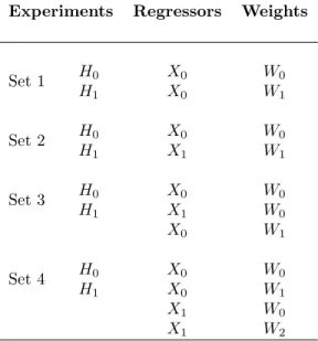
For each sample size we design four sets of experiments. In the first set of experiments the null and alternative models only differ in terms of the weighting matrix employed. In the second set the null and alternative models differ both in terms of the spatial weighting matrix and the regressor matrix. In the third and fourth set of experiments we consider more than one model under the alternative.
In the first set of experiments, the null model is generated from:
y = X0β0+λ0(IT ⊗W0)y+α0y−1+u (27)
u = N(0, σ2IN T)
where the regressors matrix X0 is taken as X0 = (x1, x2), where the N T ×1 values of x1
are generated from a uniform distribution over (0,4); theN T ×1 values of x2 are generated
from a chi-squared with three degrees of freedom.18 The elements of the parameter vectorβ0 were set to 0.5, andσ2 = 1.0; this value of σ2 lead toR2 values of, approximately 0.6. The alternative model is also generated from (27) except that it is specified in terms of the spatial weights matrix W1. In this experiment, and in the experiments below, once generated, the
values of the regressors are held fixed in the Monte Carlo trials. The parameter values, and the specification of the innovation term are given below.
18
We generate the spatial panel data with 100 +T periods and then take the lastT as our sample and we setT equal to 5 in all experiments. The initial values are generated as
In the second set of experiments, the null model is identical to (27), while the alternative model differs in terms of both the weighting matrix and the regressor matrix X1 = (z1, z2).
Specifically, the weighting matrix employed in this set of experiments isW1 (the three nearest
neighbors). Additionally, the first column of the regressors matrix (z1) is generated from an
uniform distribution over (0,3), and the values ofz2 are generated as
z2=ax1+ξ (28)
wherea = 0.5 and ξ ∼ N(0, IN T). This value of aleads to a correlation between z2 and x1
of, approximately, 0.5.
The third set of experiments is different from the previous two in that it accounts for two models under the alternative. Again, the null model is specified as in (27), and the two alternative models are specified in terms ofX0 and W1, andX1 andW0, respectively.
Finally, the fourth set of experiments accounts for three models under the alternative. While the null model is again specified as in (27), the models under the alternative are specified in terms ofX0 and W1,X1 and W0, andX1 and W2, respectively. The four sets of
experiments are summarized in Table 1.
In all four sets of experiments, six values are considered for λ, namely -0.6, -0.4, -0.2, 0.2, 0.4 and 0.6; and two values forα, namely -0.2, 0.2. Our parameter combinations are consistent with the stability conditions given in Elhorst (2001) and Parent and LeSage (2011).
The total number of combinations relating to λ, α, N and the four sets of experiment combining different definitions of W leads to a total of 6×2×2×4 = 96 experiments for each of which the two predictors are calculated. For all experiments, 2,000 replications are performed. This is roughly the number of replications needed to obtain a 95% confidence interval of length .02 on the size of a test statistic.
9
Monte Carlo Results
Our Monte Carlo results corresponding to each of the four experiments are summarized in Tables 2-9. For each experiment and sample size, these tables give the frequency of rejection of the null hypothesis at the 5% level. Reading across, the results in the first two sections give the estimated size of the test, while power estimates are given in the second two sections. The results in the tables relate to the use of our two predictors, Y(A) and Y(B). Finally, the first four tables refers to the smaller sample size (n= 100), while the other four to the larger sample size (n= 400).
Consider the results in Table 2, which are based on the first set of experiments forn= 100. Looking first at column averages, the empirical size of the test, based on both predictors in (14) is reasonably close to the theoretical 5% level. There is only one exception whenα= 0.2 and λ= 0.6. In this case the average sizes of the test corresponding to the predictor y(A) is, in percentage points, 6.15. The theoretical level, in percentage terms, is 5.00. A glance at the corresponding results in Table 6, based onn= 400, suggests that as the sample size increases the empirical size gets closer to the theoretical level.
Let us turn now to the reported power calculations of the J-test in Table 2. Again, in terms of column averages, it should be clear that theJ-test exhibits “very” high power in all cases relating to the first set of experiments in which the null and alternative models differ only in the spatial weight matrix. In these cases, the power results seem to be degraded for low values ofλ.19 Given our Monte Carlo design, the power is very high and, in general, differences relating to the use of the two predictor are small. Therefore, based on computational simplicity we suggest the use of our test in this paper based on the predictor y(A).20 When the sample
size increases (see Table 6) the power calculation are virtually all equal to 1.0. 19
In a sense this result is not very surprising given that the power of any test will depend on the extent to which the null and alternative hypotheses differ. A further discussion of this is given by LeSage and Pace (2009). Using Bayesian posterior model comparisons, they illustrate for alternative weight matrices that as the spatial dependence approaches low levels, the posterior probabilities approach the prior probabilities. In the limiting case, if the spatial dependence were zero an empirical test would not be able to distinguish between two different weighting matrices.
20However, as pointed out by Jin and Lee (2013), there might be situations where the gap in the power for
the two versions of the spatialJ-test may be large. This is an issue that could be explored in a larger Monte Carlo study, and we leave it for further research.
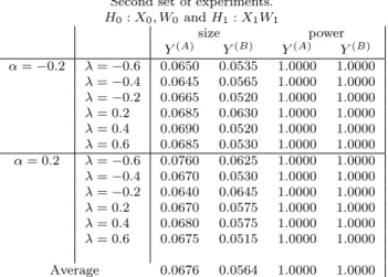
Consider now the results in Table 3, where the difference between the null and alternative model pertains to both the weighting matrix and the regressors matrix. The empirical size of the test, based on the predictory(B), is reasonably close to the theoretical 5% level. There
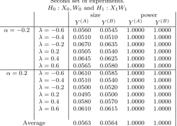
are very few exceptions mostly related to low values of λ. Specifically, these exceptions are, in percentage points, 6.3, 6.25 and 6.45. On the other hand, concerning the predictor y(A), none of the estimates of the empirical size fall into the acceptance interval (.041, .060) and the test seems to systematically over-reject the null hypothesis.21 Fortunately, we note that this “size of test problem” diminishes as the value ofn increases. In fact, looking at column averages in Table 7, we note that the empirical size of the test, based on both predictors, is reasonably close to the theoretical 5% level when the sample size isn= 400. There are a few exceptions that do not fall into the “acceptance interval”. Moving to the power of the test we observe from Table 3 that, for all combinations of model parameters, the power of the test corresponding to the use of both predictors is equal to one. The suggestion is that, in terms of power, if the null and alternative models differ in both the spatial weighting matrix and the regressor matrices, the two tests we suggest in this paper are equally good.
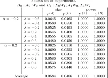
The last two sets of experiments are specified in such a way that the null model is tested against two (or more) possible alternatives. In particular, Table 4 relates to a situations where there are two models under the alternatives, while the results in Table 5 are obtained when there are three models under the alternative.
Results in Table 4 and 5 suggest that, when there is more than one model under the alternative hypothesis the empirical size of the test, based on both predictors, is reasonably close to the theoretical 5% level. Interestingly, there are no exceptions to this in Table 4. However, Table 5 presents a few cases in which the empirical sizes do not fall into the “acceptance interval”. These cases are mostly related to the use of the first predictor, and only one case relates to the second predictor. Fortunately, we note again that this “size of test problem” diminishes as the value ofnincreases. In fact, looking at Table 9, we note that there are only two individual size estimates significantly different from 5% when the sample 21Some studies have suggested to implement bootstrap testing procedure to improve the small sample
per-formance of the test (see, e.g., Burridge and Fingleton, 2010, for an example in a spatial context). We decided to leave this for future research.
size isn= 400. Finally, the reported powers in Table 4 and 5 are very high and suggest that in reasonably large samples, the two tests considered are quite “powerful”.
10
Conclusion
In this paper we extended the J-test to a spatial panel model containing fixed effects, a spatially lagged dependent variable, and a time lagged dependent variable. The disturbance term in our model was specified non-parametrically and allows for general patterns of spatial and time correlation, as well as heteroskedastity. The alternative models were specified in such a way that both spatial and time correlation of various sorts, as well as general patterns of heteroskedasticity are special cases. These alternative models can have either fixed or random effects. Given reasonable assumptions, our test is computationally simple.
We gave formal large sample results, as well as small sample Monte Carlo results that suggested, among other things, that our proposedJ-test has good power, and proper size for small to moderately sized samples.
Finally, we implemented our procedure to test the specifications of a demand for cigarette model. Our empirical results suggested that the most appropriate specification was the one involving a spatial lag of cigarette consumption in neighboring states.
One suggestion for future research would be an extension of our results to the case in
which bothN → ∞ and T → ∞. In doing this one should, among other things, account for
the possible limits ofN/T - e.g., to 0,∞, or a finite constant. Another extension would be to non-linear spatial models in a panel framework. Among others, such a framework would arise in qualitative, or limited dependent variable models. Still another suggestion for future research relates to small sample issues which would arise in a Monte Carlo study in which the true value of a parameter relating to the spatial lag of the dependent variable is “close” to a limiting value of the parameter space- e.g., if 1.0 is a limiting value then the true value might be.9.Assuming the stability conditions described in Parent and LeSage (2011), in this framework estimates of this parameter would, in some trials, exceed that upper limit. There are various ways of handling such cases but guidance on this issue would be relevant.
References
Anselin, L., Le Gallo, J., and Jayet, H. (2008). Spatial panel econometrics. In Matyas,
L. and Sevestre, P., editors, The econometrics of Panel Data, Fundamentals and Recent
Developments in Theory and Practice (3rd Edition), pages 624 – 660. Springer-Verlag, Berlin Heidelberg.
Anselin, L. and Lozano-Gracia, N. (2008). Errors in variables and spatial effects in hedonic house price models of ambient air quality. Empirical Economics, 34(1):5–34.
Baltagi, B. (2008). Econometric Analysis of Panel Data, 4th edition. Wiley, New York. Baltagi, B., Egger, P., and Pfafermayr, M. (2007a). Estimating models of complex fdi: are
there third-country effects? Journal of Econometrics, 140:260–281.
Baltagi, B., Egger, P., and Pfaffermayr, M. (2013). A generalized spatial panel data model with random effects. Econometric Reviews, 32(5 –6):650 – 685.
Baltagi, B., Kelejian, H., and Prucha, I. (2007b). Analysis of spatially dependent data.Journal of Econometrics, 140:1–4.
Baltagi, B. and Liu, L. (2008). Testing for random effects and spatial lag dependence in panel data models. Statistics and Probability Letters, 78:3304–3306.
Baltagi, B., Song, S., Jung, B., and Koh, W. (2007c). Testing for serial correlation, spatial autocorrelation and random effects using panel data. Journal of Econometrics, 140(1):5–51. Baltagi, B., Song, S., and Koh, W. (2003). Testing panel data regression models with spatial
error correlation. Journal of Econometrics, 117:123–150.
Baltagi, B. H. and Levin, D. (1986). Estimating dynamic demand for cigarettes using panel data: The effects of bootlegging, taxation and advertising reconsidered. The Review of Economics and Statistics, 68:148–155.
Baltagi, B. H. and Levin, D. (1992). Cigarette taxation: raising revenues and reducing
Burridge, P. and Fingleton, B. (2010). Bootstrap inference in spatial econometrics: the J-test.
Spatial Economic Analysis, 5:93–119.
Dastoor, N. (1983). Some Aspects of Testing Non-Nested Hypothesis. Journal of
Economet-rics, 21:213–228.
Davidson, R. and MacKinnon, J. (1981). Several tests for model specification in the presence of alternative hypotheses. Econometrica, 49:781–794.
Debarsy, N. and Ertur, C. (2010). Testing for spatial autocorrelation in a fixed effects panel data model. Regional Science and Urban Economics, 40:453–470.
Debarsy, N., Ertur, C., and LeSage, J. P. (2012). Interpreting dynamic space-time panel data models. Statistical Methodology, 9:158 – 171.
Delgado, M. and Stengos, T. (1994). Semiparametric specification testing of non-nested
econometric models. Review of Economic Studies, 61:291–303.
Elhorst, J. (2001). Dynamic models in space and time. Geographical Analysis, 33(2):119–140. Elhorst, J. (2003). Specification and estimation of spatial panel data models. International
Regional Sciences Review, 26(3):244–268.
Elhorst, J. (2008). Serial and spatial error correlation. Economics Letters, 100:422–424. Elhorst, J. (2009). Spatial panel data models. In Fischer, M. M. and Getis, A., editors,
Handbook of Applied Spatial Analysis. Springer, Berlin, Heidelberg, New York.
Elhorst, J. (2010). Dynamic panels with endogenous interactions effects when T is small.
Regional Science and Urban Economics, 40:272–282.
Elhorst, J. and Freret, S. (2009). Yardstick competition among local governments: French
evidence using a two -regimes spatial panel data model. Journal of Regional Science,
Elhorst, J., Piras, G., and Arbia, G. (2010). Growth and convergence in a multi-regional model with space-time dynamics. Geographical Analysis, 42:338–355.
Elhorst, J. P. (2005). Unconditional maximum likelihood estimation of linear and log-linear dynamic models for spatial panels. Geographical Analysis, 37:62–83.
Florax, R., Folmer, H., and Rey, S. (2003). Specification searches in spatial econometrics: the relevance of Hendry’s methodology. Regional Science and Urban Economics, 33:557–579. Godfrey, L. (1983). Testing non-nested Models After Estimation by Instrumental Variables
or Least Squares. Econometrica, 51:355–366.
Godfrey, L. and Pesaran, M. (1983). Test of non-nested regression models.Journal of Econo-metrics, 21:133–154.
Greene, W. (2003). Econometric Analysis (fifth edition). Prentice Hall, Upper Saddle River. Jin, F. and Lee, L. (2013). Cox-type tests for competing spatial autoregressive models with spatial autoregressive disturbances. Regional Science and Urban Economics, 43:590 – 616. Kapoor, M., Kelejian, H., and Prucha, I. (2007). Panel Data Model with Spatially Correlated
Error Components. Journal of Econometrics, 140(1):97–130.
Kelejian, H., Murrell, P., and Shepotylo, O. (2013). Spatial spillovers in the development of institutions. Journal of Development Economics, pages 297–315.
Kelejian, H. and Piras, G. (2011). An extension of kelejian’s j-test for non-nested spatial models. Regional Science and Urban Economics, 41:281–292.
Kelejian, H. and Prucha, I. (1999). A generalized moments estimator for the autoregressive parameter in a spatial model. International Economic Review, 40(2):509–533.
Kelejian, H. and Prucha, I. (2007). HAC estimation in a spatial framework. Journal of
Kelejian, H. H. (2008). A spatial j-test for model specification against a single or a set of nonnested alternatives. Letters in Spatial and Resources Sciences, 1(1):3–11.
Kim, M. S. and Sun, Y. (2011). Spatial heteroskedasticity and autocorrelation consistent estimation of covariance matrix. Journal of Econometrics, 160(2):349 – 371.
Kmenta, J. (1986). Elements of Econometrics (second edition). Macmillan, New York. Lee, L. and Yu, J. (2010a). Estimation of spatial autoregressive panel data models with fixed
effects. Journal of Econometrics, 154:165–185.
Lee, L. and Yu, J. (2010b). Some recent development in spatial panel data models. Regional Science and Urban Economics, 40:255–271.
Lee, L. and Yu, J. (2010c). A spatial dynamic panel data model with both time and individual fixed effects. Econometric Theory, 26:564–597.
Lee, L. and Yu, J. (2010d). A unified transformation approach to the estimation of spatial dynamic panel data models: stability, spatial cointegration and explosive roots. In A., U. and Giles, D., editors, Handbook of Empirical Economics and Finance, pages 397–434. Chapman and Hall - CRC.
LeSage, J. and Pace, K. (2009). Introduction to Spatial Econometrics. CRC Press, Boca
Raton, FL.
MacKinnon, J., White, H., and Davidson, R. (1983). Test for model specification in the pres-ence of alternative hypotheses: Some further results.Journal of Econometrics, 21(1):53–70. Mutl, J. and Pfaffermayr, M. (2011). The Hausman test in a Cliff and Ord panel model.
Econometrics Journal, 14:48–76.
Parent, O. and LeSage, J. (2010). A spatial dynamic panel model with random effects applied to commuting times. Transportation Research Part B, 44:633–645.
Parent, O. and LeSage, J. (2011). A space-time filter for panel data models containing random effects. Computational Statistics and Data Analysis, 55(1):475–490.
Pesaran, H. M. and Tosetti, E. (2011). Large panels with common factors and spatial corre-lations. Journal of Econometrics, 161(2):182 –202.
Pesaran, M. (1974). On the general problem of model selection. Review of Economic Studies, 41:153–171.
Pesaran, M. (1982). Comparison of local power of alternative tests of non-nested regression models. Econometrica, 50:1287–1305.
Pesaran, M. and Deaton, A. (1978). Testing non-nested non-linear regression models. Econo-metrica, 46:677–694.
Pesaran, M. and Weeks, M. (2001). Non-nested hypothesis testing: an overview. In Baltagi, B., editor,A companion to theoretical econometrics. Blackwell, Malden.
Piras, G. (2013). Efficient gm estimation of a cliff and ord panel data model with random effects. Spatial Economic Analysis, forthcoming.
P¨otscher, B. M. and Prucha, I. R. (2000). Basic elements of asymptotic theory. In Baltagi, B. H., editor,A Companion to Theoretical Econometrics, pages 201 – 229. Basil Blackwell. Yu, J., de Jong, R., and Lee, L. (2008). Quasi maximum likelihood estimators for spatial dynamic panel data with fixed effects when both n and t are large.Journal of Econometrics, 146:118–134.
Yu, J. and Lee, L. (2010). Estimation of unit root spatial dynamic panel data models.
Table 1: Experimental Designs Relating to the Regressor and Weighting Matrices
Experiments Regressors Weights
Set 1 H0 X0 W0 H1 X0 W1 Set 2 H0 X0 W0 H1 X1 W1 Set 3 H0 X0 W0 H1 X1 W0 X0 W1 Set 4 H0 X0 W0 H1 X0 W1 X1 W0 X1 W2
Table 2: Frequency of rejection of the null hypothesis: two predictors (2000 replications), n= 100, t= 5.
First set of experiments.
H0:X0, W0 andH1:X0W1 size power Y(A) Y(B) Y(A) Y(B) α=−0.2 λ=−0.6 0.0505 0.0525 1.0000 1.0000 λ=−0.4 0.0500 0.0510 1.0000 1.0000 λ=−0.2 0.0540 0.0545 0.8885 0.8985 λ= 0.2 0.0495 0.0450 0.9155 0.8655 λ= 0.4 0.0560 0.0565 1.0000 1.0000 λ= 0.6 0.0555 0.0590 1.0000 1.0000 α= 0.2 λ=−0.6 0.0575 0.0525 1.0000 1.0000 λ=−0.4 0.0515 0.0435 1.0000 1.0000 λ=−0.2 0.0475 0.0525 0.8405 0.8510 λ= 0.2 0.0580 0.0595 0.8475 0.7670 λ= 0.4 0.0445 0.0450 1.0000 1.0000 λ= 0.6 0.0615 0.0565 1.0000 1.0000 Average 0.0530 0.0523 0.9577 0.9485
Table 3: Frequency of rejection of the null hypothesis: two predictors (2000 replications), n= 100, t= 5.
Second set of experiments.
H0:X0, W0 andH1:X1W1 size power Y(A) Y(B) Y(A) Y(B) α=−0.2 λ=−0.6 0.0650 0.0535 1.0000 1.0000 λ=−0.4 0.0645 0.0565 1.0000 1.0000 λ=−0.2 0.0665 0.0520 1.0000 1.0000 λ= 0.2 0.0685 0.0630 1.0000 1.0000 λ= 0.4 0.0690 0.0520 1.0000 1.0000 λ= 0.6 0.0685 0.0530 1.0000 1.0000 α= 0.2 λ=−0.6 0.0760 0.0625 1.0000 1.0000 λ=−0.4 0.0670 0.0530 1.0000 1.0000 λ=−0.2 0.0640 0.0645 1.0000 1.0000 λ= 0.2 0.0670 0.0575 1.0000 1.0000 λ= 0.4 0.0680 0.0575 1.0000 1.0000 λ= 0.6 0.0675 0.0515 1.0000 1.0000 Average 0.0676 0.0564 1.0000 1.0000
Table 4: Frequency of rejection of the null hypothesis: two predictors (2000 replications), n= 100, t= 5.
Third set of experiments.
H0:X0, W0andH1:X0W1;X1W0 size power Y(A) Y(B) Y(A) Y(B) α=−0.2 λ=−0.6 0.0575 0.0580 1.0000 1.0000 λ=−0.4 0.0510 0.0485 1.0000 1.0000 λ=−0.2 0.0430 0.0460 1.0000 1.0000 λ= 0.2 0.0540 0.0445 1.0000 1.0000 λ= 0.4 0.0490 0.0410 1.0000 1.0000 λ= 0.6 0.0510 0.0460 1.0000 1.0000 α= 0.2 λ=−0.6 0.0475 0.0495 1.0000 1.0000 λ=−0.4 0.0545 0.0490 1.0000 1.0000 λ=−0.2 0.0540 0.0470 1.0000 1.0000 λ= 0.2 0.0485 0.0415 1.0000 1.0000 λ= 0.4 0.0570 0.0445 1.0000 1.0000 λ= 0.6 0.0440 0.0465 1.0000 1.0000 Average 0.0509 0.0468 1.0000 1.0000
Table 5: Frequency of rejection of the null hypothesis: two predictors (2000 replications), n= 100, t= 5.
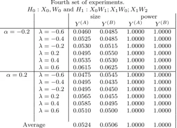
Fourth set of experiments.
H0:X0, W0andH1:X0W1;X1W0;X1W2 size power Y(A) Y(B) Y(A) Y(B) α=−0.2 λ=−0.6 0.0645 0.0465 1.0000 1.0000 λ=−0.4 0.0580 0.0550 1.0000 1.0000 λ=−0.2 0.0525 0.0495 1.0000 1.0000 λ= 0.2 0.0545 0.0460 1.0000 1.0000 λ= 0.4 0.0555 0.0505 1.0000 1.0000 λ= 0.6 0.0480 0.0450 1.0000 1.0000 α= 0.2 λ=−0.6 0.0625 0.0510 1.0000 1.0000 λ=−0.4 0.0690 0.0555 1.0000 1.0000 λ=−0.2 0.0680 0.0505 1.0000 1.0000 λ= 0.2 0.0580 0.0505 1.0000 1.0000 λ= 0.4 0.0530 0.0390 1.0000 1.0000 λ= 0.6 0.0575 0.0440 1.0000 1.0000 Average 0.0584 0.0486 1.0000 1.0000
Table 6: Frequency of rejection of the null hypothesis: two predictors (2000 replications), n= 400, t= 5.
First set of experiments.
H0:X0, W0 andH1:X0W1 size power Y(A) Y(B) Y(A) Y(B) α=−0.2 λ=−0.6 0.0515 0.0490 1.0000 1.0000 λ=−0.4 0.0520 0.0535 1.0000 1.0000 λ=−0.2 0.0480 0.0460 1.0000 1.0000 λ= 0.2 0.0430 0.0445 1.0000 1.0000 λ= 0.4 0.0520 0.0505 1.0000 1.0000 λ= 0.6 0.0555 0.0510 1.0000 1.0000 α= 0.2 λ=−0.6 0.0465 0.0445 1.0000 1.0000 λ=−0.4 0.0530 0.0535 1.0000 1.0000 λ=−0.2 0.0500 0.0500 1.0000 1.0000 λ= 0.2 0.0455 0.0480 1.0000 1.0000 λ= 0.4 0.0465 0.0445 1.0000 1.0000 λ= 0.6 0.0490 0.0510 1.0000 1.0000 Average 0.0494 0.0488 1.0000 1.0000
Table 7: Frequency of rejection of the null hypothesis: two predictors (2000 replications), n= 400, t= 5.
Second set of experiments.
H0:X0, W0 andH1:X1W1 size power Y(A) Y(B) Y(A) Y(B) α=−0.2 λ=−0.6 0.0560 0.0545 1.0000 1.0000 λ=−0.4 0.0510 0.0510 1.0000 1.0000 λ=−0.2 0.0670 0.0635 1.0000 1.0000 λ= 0.2 0.0505 0.0540 1.0000 1.0000 λ= 0.4 0.0645 0.0625 1.0000 1.0000 λ= 0.6 0.0565 0.0580 1.0000 1.0000 α= 0.2 λ=−0.6 0.0610 0.0585 1.0000 1.0000 λ=−0.4 0.0510 0.0540 1.0000 1.0000 λ=−0.2 0.0500 0.0520 1.0000 1.0000 λ= 0.2 0.0495 0.0500 1.0000 1.0000 λ= 0.4 0.0580 0.0570 1.0000 1.0000 λ= 0.6 0.0610 0.0615 1.0000 1.0000 Average 0.0563 0.0564 1.0000 1.0000
Table 8: Frequency of rejection of the null hypothesis: two predictors (2000 replications), n= 400, t= 5.
Third set of experiments.
H0:X0, W0andH1:X0W1;X1W0 size power Y(A) Y(B) Y(A) Y(B) α=−0.2 λ=−0.6 0.0455 0.0470 1.0000 1.0000 λ=−0.4 0.0475 0.0505 1.0000 1.0000 λ=−0.2 0.0530 0.0610 1.0000 1.0000 λ= 0.2 0.0505 0.0490 1.0000 1.0000 λ= 0.4 0.0450 0.0550 1.0000 1.0000 λ= 0.6 0.0545 0.0540 1.0000 1.0000 α= 0.2 λ=−0.6 0.0460 0.0480 1.0000 1.0000 λ=−0.4 0.0540 0.0590 1.0000 1.0000 λ=−0.2 0.0560 0.0580 1.0000 1.0000 λ= 0.2 0.0470 0.0470 1.0000 1.0000 λ= 0.4 0.0490 0.0475 1.0000 1.0000 λ= 0.6 0.0500 0.0535 1.0000 1.0000 Average 0.0498 0.0525 1.0000 1.0000
Table 9: Frequency of rejection of the null hypothesis: two predictors (2000 replications), n= 400, t= 5.
Fourth set of experiments.
H0:X0, W0andH1:X0W1;X1W0;X1W2 size power Y(A) Y(B) Y(A) Y(B) α=−0.2 λ=−0.6 0.0460 0.0485 1.0000 1.0000 λ=−0.4 0.0525 0.0485 1.0000 1.0000 λ=−0.2 0.0530 0.0515 1.0000 1.0000 λ= 0.2 0.0495 0.0550 1.0000 1.0000 λ= 0.4 0.0535 0.0530 1.0000 1.0000 λ= 0.6 0.0615 0.0625 1.0000 1.0000 α= 0.2 λ=−0.6 0.0475 0.0545 1.0000 1.0000 λ=−0.4 0.0495 0.0435 1.0000 1.0000 λ=−0.2 0.0495 0.0450 1.0000 1.0000 λ= 0.2 0.0565 0.0455 1.0000 1.0000 λ= 0.4 0.0585 0.0495 1.0000 1.0000 λ= 0.6 0.0510 0.0500 1.0000 1.0000 Average 0.0524 0.0506 1.0000 1.0000
Table 10: Estimation of the alternative model.
Coefficients se t-stat p-val lnpi,t -0.4366 0.0454 -9.6174 0.0000 lnIi,t 0.1661 0.0316 5.2492 0.0000 PN j=1wijlnpj,t 0.1776 0.0974 1.8237 0.0682 PN j=1wijlnCj,t 0.2169 0.0564 3.8440 0.0001 lnCi,t−1 0.6433 0.0371 17.3191 0.0000
Table 11: Estimation of the null model.
Coefficients se t-stat p-val lnpi,t -0.4957 0.0492 -10.0726 0.0000
lnIi,t 0.1894 0.0361 5.2467 0.0000
lnpmin -0.0159 0.0359 -0.4441 0.6569
lnCi,t−1 0.6016 0.0410 14.6690 0.0000
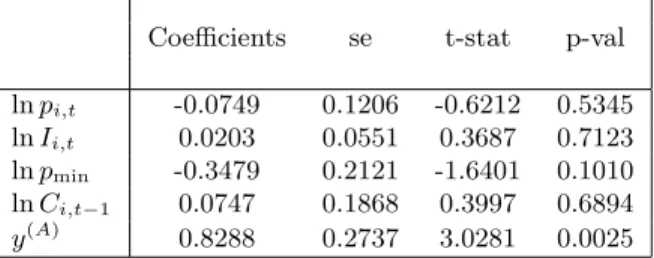
Table 12: Estimation of the augmented model using the first predictor y(A) based on the
minimum information set.
Coefficients se t-stat p-val lnpi,t -0.0749 0.1206 -0.6212 0.5345
lnIi,t 0.0203 0.0551 0.3687 0.7123
lnpmin -0.3479 0.2121 -1.6401 0.1010
lnCi,t−1 0.0747 0.1868 0.3997 0.6894
Appendix
A: Asymptotic equivalence of Q0YJE,A and Q0YJE,B when G= 1
A.1: Results relating to
z }| { Q0YJE,A
Let
Q0 = [Q00,1, ..., Q00,T]0
whereQ0,t is theN×N T matrix which consists of thetth block ofN consecutive rows ofQ0
- e.g., Q0,1is the first N consecutive rows of Q0, etc. Let Q0,t,i. be the ith row of Q0,t and
note from (10) and (11) thatE[Q0,t,i.y|H1,J, IN F OJ,tmax] =Q0,t,i.E[y|H1,J, IN F OJ,tmax] where
Q0,t,i.E[y|H1,J, IN F OJ,tmax] = Q0,t,i.MJφ1,J +Q0,t,i.P φ2,J (29)
+λJQ0,t,i.0(IT ⊗WJ)y+αJQ0,t,i.y−1
+Q0,t,i.E[νJ|H1,J, IN F OmaxJ,t ]
Let
rJ|t,i =Q0,t,i.E[νJ|H1,J, IN F OJ,tmax] (30)
and note thatrJ|t,i 6= 0 since the elements of theN T×1 vectorνJ are both spatially and time
correlated, andIN F OmaxJ,t contains the vectors [y0, ..., yt−1, y−i,t]. However, using the iterated
expectations principle, recalling thatIN F Omax
J,t contains ΥJ = (MJ, P, WJ),and Assumption
2 it follows that
E[rJ|t,i|H1,J,ΥJ] = Q0,t,i.E[E(νJ|H1,J, IN F OJ,tmax)|H1,J,ΥJ] (31)
= Q0,t,i.E(νJ|H1,J,ΥJ) = 0
The results in (30) and (31) imply
whereE[ΘJ|t,i|H1,J,ΥJ] = 0.22
LetrJ|t= [rJ|t,1, ..., rJ|t,N]0 and rJ = [rJ|1, ..., rJ|T]0. It follows from (30) - (32) that
Q0νJ =rJ + ΘJ (33)
where
E[Q0νJ|H1,J,ΥJ] =E[rJ|H1,J,ΥJ] =E[ΘJ|H1,J,ΥJ] = 0 (34)
and the VC matrix of Q0νJ is
Q0VvJQ0 =VrJ +VΘJ +CrJ,ΘJ +C
0
rJ,ΘJ (35)
where VrJ and VΘJ are, respectively, the variance covariance matrices of rJ and ΘJ, and CrJ,ΘJ is the covariance matrix between rJ and ΘJ. Clearly the row and column sums of Q0 are uniformly bounded in absolute value by TT−1 <2.0; By Assumption 2, the row and
column sums of VvJ are also uniformly bounded in absolute value. Since the product of
matrices whose row and column sums are uniformly bounded in absolute value also have rows and column sums which are so uniformly bounded, the row and column sums ofQ0VvJQ0 are
also uniformly bounded in absolute value. It then follows from (35) that the row and column sums ofVrJ are uniformly bounded in absolute value.
IfrJwere observed and used, the predictor
z }| {
Q0YJE,Ain (14) would be replaced by
z }| { Q0YJE,A+rJ
in the augmented regression (16). We now show that the large sample distribution of ˜ξi in (18) does not involverJ.
The estimator ˜ξi can be expressed
(N T)1/2[˜ξi−ξi] = N T( ˜Φ0iΦ˜i)−1(N T−1/2) ˜Φ0iQ0Rε (36) = n [(N T)−1Φˆ0iH] [(N T)(H0H)−1] [(N T)−1H0Φˆi] o−1 ∗ [(N T)−1Φˆ0iH] [(N T)(H0H)−1] [(N T)−1/2H0Q0Rε]
22To see this, take expectations across in (32) conditional onH
Since ˆΦA = Q0ΓˆA and, in this case ˆΓA = [Z,
z }| {
Q0YJE,A+rJ], the term rJ only arises in (36)
in terms of the product (N T)−1H0Q0[Z,
z }| {
Q0YJE,A+rJ]. Let ηJ = (N T)−1H0Q0rJ. Then, in
light of (36) the termrJ enters into the large sample distribution of ˜ξi only viaηJ. It follows
from (33) - (35) that the mean and variance covariance matrix ofηJ are
E[ηJ|H1,J,ΥJ] = 0 (37)
E[ηη0J|H1,J,ΥJ] = (N T)−2H0[Q0VrJQ0]H
In light of (35) the row and column sums of Q0VrJQ0 are uniformly bounded in absolute
value. By Assumption 4, the elements ofH are uniformly bounded in absolute value and so the elements ofH0[Q0VrJQ0]H are 0(N); it follows from (37) that
E[ηη0J|H1,J,ΥJ]→0 (38)
The results in (37), (38), and Chebyshev’s inequality imply
ηJ →P 0 (39)
It then follows that, asymptotically,rJ is of no consequence in our J-test.
A.2: Equivalence of Q0YJE,A and Q0YJE,B, asymptotically, when G= 1.
Let
KJ = [IT ⊗(IN−λJWJ)−1] (40)
and note from (8) and (10) that underH1,J
ConsiderQ0YJEA and, recalling (8) and (13), we have
Q0YJE,A = Q0MJφ1,J +Q0P φ2,J+λJ(IT ⊗WJ)Q0y+αJQ0y−1 (42)
= Q0MJφ1,J +Q0P φ2,J+αJQ0y−1+ (IT ⊗λJWJ)∗
[KJQ0MJφ1,J+KJQ0P φ2,J +αJKJQ0y−1+KJQ0νJ]
Combining terms in (42) we have
Q0YJE,A=SJQ0MJφ1,J +SJQ0P φ2,J +SJQ0y−1λJ+ (IT ⊗λJWJ)KJQ0vJ (43) where SJ = IN T + (IT ⊗λJWJ) (IT ⊗(IN −λJWJ)−1) (44) = [IT ⊗(IN−λJWJ) + (IT ⊗λJWJ)] [IT ⊗(IN −λJWJ)−1] = IT ⊗(IN −λJWJ)−1 ≡ ΠJ, J= 1, ..., G
where ΠJ is defined in (12). LethJ = (IT ⊗λJWJ)KJQ0vJ. It then follows from (42) - (44)
that
Q0YJE,A = ΠJQ0MJφ1,J + ΠJQ0P φ2,J + ΠJQ0y−1λJ +hJ (45)
≡ Q0YJE,B+hJ
sinceQ0ΠJ = ΠJQ0. Thus, in finite samples the only difference between the use ofYJE,A and
YJE,B is the term hJ. However, asymptotically, hJ is of no consequence for the same reason
that rJ is of no consequence. For example, it follows from (36) that hJ can only effect the
asymptotic distribution of ˜ξi ifplimN→∞(N T)−1H0hJ 6= 0. However, (N T)−1H0hJ P
sohJ is of no consequence. To see this, let ΨJ = (N T)−1H0hJ. Now note from (34) that E[ΨJ|H1,J,ΥJ] = (N T)−1H0(IT ⊗λJWJ)KJQ0E[vJ|H1,J,ΥJ] (46) = 0 and E[ΨJΨ0J|H1,J,ΥJ] = (N T)−2H0[(IT ⊗λJWJ)KJ][Q0VvJQ0][K 0 J(IT ⊗λJWJ0)]H (47)
It follows from Assumption 3 and (35) that the row and column sums of the matrices in brackets in (47) are uniformly bounded in absolute value; in addition, from Assumption 4 the elements of H are uniformly bounded in absolute value. Therefore, the elements of the VC matrixE[ΨJΨ0J|H1,J,ΥJ] are 0(N−1) and soE[ΨJΨ0J|H1,J,ΥJ]→0.Chebyshev’s inequality
then implies that ΨJ →P 0.
Of course, in practice
z }| { Q0YJE,Aand
z }| {
Q0YJE,Bwould be used instead ofQ0YJE,AandQ0YJE,B.
Therefore the use of
z }| { Q0YJE,A and
z }| {
Q0YJE,B would be asymptotically equivalent if, in light
of (36), the data and estimation procedure associated withH1,J are such that the parameters
are consistently estimated and
p lim N→∞(N T) −1H0z }| { Q0YJE,A=p lim N→∞(N T) −1H0 Q0YJE,A (48) p lim N→∞(N T) −1H0zQ }| { 0YJE,B =p lim N→∞(N T) −1H0Q 0YJE,B Proof of Theorem 1
To simplify notation, we prove Theorem 1 for the case in which
z }| {
Q0YJE,Ais used, J =
1, ..., G.The proof for the case in which
z }| {
First note from (10), (14) and (15) that
ˆ
Y1A,G = [Z1, ..., ZG] [ˆγ01, ...,γˆ0G]0 (49)
= Z1,G γˆ1,G
whereZ1,G = [Z1, ..., ZG] and ˆγ1,G= [ˆγ01, ...,ˆγ0G]0 where ˆγ0J = (ˆφ
0
1,J,φˆ
0
2,J,λˆJ,αˆJ), J = 1, ..., G.
For this case ˆΓAin (16) is
ˆ
ΓA = [Z, Z1,G ˆγ1,G] (50)
and ΓA = [Z, Z1,G γ1,G]. Therefore, recalling that ˜ΦA = PHΦˆA and ˆΦA = Q0ΓˆA it follows
from (16) and (18) that
(N T)1/2[˜ξi−ξi] = n (N T)−1ΓˆA0 Q0H [(N T)−1H0H]−1(N T)−1H0Q0ΓˆA o−1 ∗ (N T)−1ΓˆA0 Q0H (N T)(H0H)−1 (N T)−1/2H0Q0Rε (51)
Consider the term (N T)−1H0Q
0ΓˆA in the inverse on the first line of (51) and note that by
Assumption 5, ˆγ1,G →P C1,G = (c01, ..., c0G)0, where c0J = (c0,J, c2,J, LJ, aJ), J = 1, ..., G. Part
(b) of Assumption 6, and (49), imply
(N T)−1H0Q0ΓˆA] = p lim N→∞(N T) −1H0 Q0[Z, Z1,G γˆ1,G] (52) = [p lim N→∞(N T) −1H0Q 0Z, (p lim N→∞(N T) −1H0Q 0Z1,G) p lim N→∞γˆ1,G] = [p lim N→∞(N T) −1H0Q 0Z, (p lim N→∞(N T) −1H0Q 0Z1,G) γ1,G] = p lim N→∞(N T) −1H0 Q0ΓA = ΩHQ0ΓA
Let ˆzbe the inverse term on the first line of (51) and let
˜
z= ˆz∗[(N T)−1Γˆ0AQ0H] [(N T)(H0H)−1] (53)
Then from (52), and parts (a) and (b) of Assumption 6, first note that
ˆ z→P Ω0HQ0ΓAΩ −1 HHΩHQ0ΓA −1 (54) where Ω0HQ0Γ AΩ −1
HHΩHQ0ΓA is positive definite and, therefore, nonsingular since ΩHH is
pos-itive definite and so, therefore, is Ω−HH1 , and ΩHQ0ΓA has full column rank. It then follows
from (52) - (54), and and parts (a) and (b) of Assumption 6 that
˜ z→P z∗ (55) z∗ = Ω0HQ0ΓAΩ −1 HHΩHQ0ΓA −1 Ω0HQ0ΓAΩ−HH1
Finally, consider the last term on the second line in (51), namely (N T)−1/2H0Q0Rε.Since
the row and column sums of bothQ0 andRare uniformly bounded in absolute value, the row
and column sums ofQ0Rare also uniformly bounded in absolute value. Since by Assumption
4 (a) the elements ofH are uniformly bounded in absolute value it follows that the elements of H0Q0R are uniformly bounded in absolute value. Given this, and Assumptions 1, 6 part
(c), and the central limit theorem (30) in P¨otscher and Prucha (2000) it follows that
(N T)−1/2H0Q0Rε
D
→N(0,ΩH0Q
0RR0Q0H) (56)
Therefore, by the continuous mapping theorem and (51) - (55)
(N T)1/2[˜ξi−ξi]→D N(0,z∗ΩH0Q
0RR0Q0Hz
∗0