Conservative Systems 6 1

6

Conservative

TABLE OF CONTENTS

Page §6.1 Introduction . . . 6–3 §6.2 Work and Work Functions . . . 6–3 §6.2.1 Mechanical Work Concept . . . 6–3 §6.2.2 Power . . . 6–4 §6.2.3 Conservative Forces and Potential Energy . . . 6–4 §6.2.4 Work Under Multiple Forces . . . 6–5 §6.2.5 Work in a Force Field . . . 6–5 §6.2.6 Work Associated With Multiple Points . . . 6–6 §6.2.7 Separation Into Internal and External . . . 6–6 §6.3 Force Residual of Conservative Systems . . . 6–7 §6.3.1 Advantages of Energy-Based Derivations . . . 6–7 §6.4 External Work Functions . . . 6–8 §6.4.1 Point Loads . . . 6–8 §6.4.2 Distributed Dead Loads . . . 6–9 §6.5 Internal Energy Functions . . . 6–9 §6.5.1 A Linear Spring . . . 6–9 §6.5.2 A Geometrically Nonlinear Spring . . . 6–10 §6.5.3 A Spring-Propped Inverted Pendulum . . . 6–12 §6.5.4 Internal Energy Additivity Property . . . 6–13 §6.6 *Work Derivatives . . . 6–13 §6.6.1 *Work Taylor Series . . . 6–14 §6.6.2 *Work Hessians and Dual Forms . . . 6–14 §6.6.3 *Work Increments . . . 6–15 §6. Notes and Bibliography . . . 6–16 §6. Exercises . . . 6–17

§6.2 WORK AND WORK FUNCTIONS §6.1. Introduction

This Chapter treats topics pertaining to energy methods for conservative systems in a more detailed manner. The concepts of work and energy are introduced, along with potential functions. This is followed by several examples involving very simple conservative systems, which show, in step by step fashion, how to construct work functions. The last two example of this series illustrate how geometric nonlinearities naturally arise when large motions are considered.

The Chapter concludes with mathematical derivations that will be of use in the study of incremental solution methods. Such derivations are considered advanced material. This means that are not covered during the course, although key results (for example, amplification matrices) are quoted and applied in later Chapters.

§6.2. Work and Work Functions

The following definition appears in scienceworld.wolfram.com. A conservative system is one in which work done by a force, or set of forces, is

1. Independent of path.

2. Equal to the difference between the final and initial values of an energy function. 3. Completely reversible.

These three definitions can be shown to be mathematically equivalent,1 _{and are elucidated in the} following subsections.

Remark 6.1. Two practically important examples are gravitational and electrical fields. For example, in the case of a uniform gravity field, the gravitational potential energy acquired or lost by a mass depends only on the difference between heights, and not on the path taken to get from one state to the other.

§6.2.1. Mechanical Work Concept

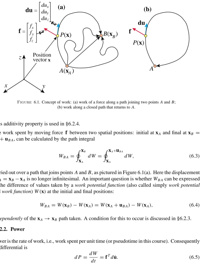
The concept of mechanical work can be elementary brought up as follows. Mechanical force f, located at position coordinate x, displaces an infinitesimal distance du, to x+du. See Figure 6.1(a). The Cartesian components of f are fx, fy, fz, whereas those of du are{dux,duy,duz}. The work differential is defined as the inner product

d W =fT du= fxdux + fyduy+ fzduz, (6.1)

in which W denotes work.2 From the definition it is obvious that mechanical work is a scalar with physical dimension of force times length. Since forces add vectorially, work differentials add algebraically. If f is the resultant of, say, f1, f2, and f3, then

d W =fTdu =(f1+f2+f3)Tdu =fT1 du+f

T

2 du+f

T

3 du= d W1+d W2 +d W3. (6.2) 1 _{The Wikipedia definition is similar: “A force is conservative if the work done by a particle between two points is} independent of the path taken. Equivalently, if a particle travels in a closed loop, the net work done is zero.” The Wiki definition has a Physics flavor as it focus on one particle; for engineering systems like structures, replace “particle” by “system,” “travel” by “motion” and “point” by “state.”

2 _{In the differential-of-work definition (6.1), du could be substituted by dx. Use of the displacement, however, fits better} within the usual nomenclature of the Finite Element Method.

P(x)

P(x)

A(x )

B(x )

(a)

A

(b)

x

y

z

du

du

f

f

Figure 6.1. Concept of work: (a) work of a force along a path joining two points A and B;

(b) work along a closed path that returns to A.

This additivity property is used in §6.2.4.

The work spent by moving force f between two spatial positions: initial at xA and final at xB =

xA+uB A, can be calculated by the path integral WB A = xB xA d W = xA+uB A xA d W, (6.3)

carried out over a path that joins points A and B, as pictured in Figure 6.1(a). Here the displacement uB A =xB−xAis no longer infinitesimal. An important question is whether WB Acan be expressed

as the difference of values taken by a work potential function (also called simply work potential and work function) W(x)at the initial and final positions:

WB A =W(xB)−W(xA)=W(xA+uB A)−W(xA), (6.4) independently of the xA →xB path taken. A condition for this to occur is discussed in §6.2.3.

§6.2.2. Power

Power is the rate of work, i.e., work spent per unit time (or pseudotime in this course). Consequently its differential is

d P = d W dt =f

T_{du˙. (6.5)}

The total power spent is obtained by the line integral of P, also called path integral, which has been introduced in the previous subsection.

§6.2 WORK AND WORK FUNCTIONS §6.2.3. Conservative Forces and Potential Energy

A force f =f(x)that is a function of position x, but independent of time, is called conservative if it is the gradient of a work potential function W(x)≡ W(u):

f= ∇W =∂_∂W_x ∂_∂W_y ∂_∂W_z T = _∂ W ∂ux ∂W ∂uy ∂W ∂uz T . (6.6)

in which∇W denotes the gradient (a column vector) of W . If (6.6) holds, the differential of work d W as defined in (6.1) is d W =(∇W)T du= ∂W ∂ux dux + ∂ W ∂uy duy+ ∂ W ∂uz duz. (6.7)

This is now an exact differential, and consequently the path integral (6.3) evaluates to (6.4) inde-pendently of the xA →xBpath. If a work potential exists, the negated function

V = −W, (6.8)

is called the potential energy function or simply potential energy, associated with the force f = −∇V . The name arises from the fact that energy is the capacity to do work. If WB A = W(xB)− W(xA)is negative, VB A = V(xB)−V(xA)= −WB A is positive, so energy has been stored when

moving the force from A to B. If B and A coalesce so that the path returns to A, as pictured in Figure 6.1(b), the net work spent, or energy stored, is zero.

Any force that cannot be expressed as (6.6) is called nonconservative.

What happens if the gradient (6.6) vanishes? Then f=0. If the system consists of just the particle at point P, it is in static equilibrium. The generalization to an arbitrary conservative system links the total force residual r to the gradient of a total potential energy, as covered in §6.3.

If all forces acting on a mechanical system are conservative, the system is called conservative, and nonconservative otherwise. Often the acting forces can be decomposed into conservative and nonconservative, as discussed in the last Chapters. For example a moving vehicle under gravity forces (conservative) and aerodynamic forces (nonconservative).

§6.2.4. Work Under Multiple Forces

Suppose that point P in Figure 6.1(a) is acted upon by several concurrent forces, say f1, f2 and f3. Then the work differential can be expanded as in equation (6.2), which is reproduced for convenience:

d W =f₁Tdu+f₂T du+f₃T du=(f₁T +f₂T +f₃T)du=fTdu. (6.9) Here f is the vectorial resultant f=f1+f2+f3. It follows that multiple forces acting at one point may be replaced by their resultant without modifying the work function. This is a consequence of the additivity of energy, a property discussed in ? in more detail.

§6.2.5. Work in a Force Field

A force-per-unit-volume (force density) that depends on position is called a field. Well known examples are gravity, centrifugal and electrostatic fields. In this case the force f acting on a body is obtained by integrating the force field over the volume of the body. For example, consider a gravity field of constant magnitude g directed along the−z axis. Suppose that a body in this field occupies the domainand has constant mass densityρ. Then the acting force in terms of components is

f= ₀ 0 ρ (−g)d = ₀ 0 −ρg d = ₀ 0 −ρg V , (6.10)

in which V = d denotes the volume measure. A similar scheme can be used for position-dependent fields, although integrals can become more complicated. The force field is called con-servative if the integrated forces over an arbitrary body are.

§6.2.6. Work Associated With Multiple Points

This scenario arises when a continuous system is discretized into a model with arbitrary number of degrees of fredom (DOF) assigned to multiple locations. If the discretization is done by the Finite Element Method (FEM) those locations are called nodes. The assignment of forces to nodes is carried out by techniques collectively known as force lumping. These are covered in the introductory FEM course [263]. The total work differential is then computed by adding up nodal force contributions.

§6.2.7. Separation Into Internal and External

This generalization is the most important one for conservative systems that involve flexible bodies. That is, bodies capable of deforming and are modeled as continua. Work is separated into two components, which together form the total potential energy function defined as

=U −W. (6.11)

Here U is the internal energy or stored energy whereas W is the work potential function of applied or external forces, introduced in §6.2.3. The internal energy is that mechanically stored in the body as a result of its deformation under stress, which ultimately (at the molecular scale) resolves into interatomic forces.3 This separation is convenient for various reasons, both physical and computational, which are explained later.

Frequently asked question: why do U and W appear with different signs in (6.11)? Physical reason: U is an energy, that is, the capacity to do work, whereas W is work spent. Take the gradient: ∇ = ∇U − ∇W , each of which has interpretation as force. For force equilibrium: ∇ =0 or∇U = ∇W . This expresses force balance: internal forces∇U balance external force ∇W ; this concept was introduced in Chapter 3 through the residual split (3.4).

If W is replaced by−V as per (6.8), takes the form

=U +V. (6.12)

3 _{Other components of internal energy, for example those associated with thermomechanical, electromagnetic, or chemical} reaction (such as combustion) effects, are not considered here.

§6.3 FORCE RESIDUAL OF CONSERVATIVE SYSTEMS This states that the total energy of the system is the sum of the internal and external energies. Although (6.12) is philosophically easier to grasp, it is not popular in FEM formulations because the idea of force balance takes precedence there. However, form (6.12) is used more frequently in Lagrangian and Hamiltonian dynamics to express total-energy conservation laws.

§6.3. Force Residual of Conservative Systems

The concepts introduced in in §6.2 justify the linkage of force residuals to energy functions. This connection was introduced in previous Chapters as recipes, but can now be restated in a more systematic form. The total residual force vector r may be expressed as the gradient of the total potential energy with respect to the state vector. For the case of multiple control parameters covered in Chapter 3:

r(u,Λ)= ∂ (u,Λ)

∂u , (6.13)

whereas for the case of a single control parameter (the staging parameter), introduced in Chapter 4:

r(u, λ)= ∂ (u, λ)

∂u , (6.14)

Furthermore, the energy and force decompositions = U −W and r = p−f are related in the sense that

p= ∂U

∂u, f=

∂W

∂u . (6.15)

in which p and f are the internal and external forces, respectively.

The force equilibrium equations r =0 or f=p express the fact that the total potential energy is

stationary with respect to variations of the state vector when the structure is in static equilibrium. Mathematically: δ =rTδu= ∂ ∂u T δu=0. (6.16)

whereδu denotes a virtual displacement,4δbeing the variation symbol. Sinceδu is arbitrary, (6.16) implies that r=0.

§6.3.1. Advantages of Energy-Based Derivations

If the structural system is conservative there are several advantages in taking advantage of that property:

(1) If discrete force equilibrium equations are worked out by hand (either for complete structures or finite elements) derivation from a potential is usually simpler than direct use of equilibrium (for example, using Free Body Diagrams), because differentiation is a straightforward and less error prone operation, especially as regards getting correct signs.5

4 _{An infinitesimal displacement compatible with the kinematic constraints. A virtual displacement is not necessarily the} same as an actual displacement.

5 _{For complicated energy gradient derivations, a computer algebra system (CAS) can be used to reduce the chance for} errors by making differentation automatic.

(2) The transformation of residual equations to different coordinate systems is simplified because of the invariance properties of energy functions. Namely, does not depend on the choice of coordinates. If those change, simply update the DOF in the partial derivatives.

(3) The conventional FEM relies on the availability of energy functionals because the additivity property is essential: the total energy of the system is the sum of the element energies. (4) The tangent stiffness matrix is guaranteed to be symmetric. Consequently equation solvers

(as well as eigensolvers) can take advantage of this property.

(5) Loss of stability can be assessed by the singular stiffness criterion introduced in Chapter 5, That criretion is static in nature. If the system is nonconservative, loss of stability may have to be tested by a dynamic criterion, which can be error-prone and computationally expensive. §6.4. External Work Functions

In mechanics, the concept of load potential is the easiest to explain, because the idea of work as force times displacement is introduced in early Physics courses. This function, called W , is the potential of the work done by the applied or prescribed forces working on the displacements of the points on which those forces act. As discussed in §6.2.7, the egated function V = −W is called the external potential function, but in the present course we shall primarily use W .

Next we illustrate how to build W for systems with finite degrees of freedom. The presentation is not general in nature but relies on a few simple examples complemented with exercises. The material is intended to serve as a “bridge” to the formulation of geometrically nonlinear finite elements, which starts in Chapter 9.

§6.4.1. Point Loads

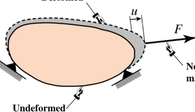
For a concrete example, consider a structure loaded by a single point force F that does not change in magnitude or direction as the structure displaces. See Figure 6.2. A force with these properties is called a dead load. If u is the displacement of the point of application of F in the direction of the force, then the work performed is obviously F u. Consequently,

W = F u. (6.17)

If the structure is subjected to n loads Fk (k = 1, . . .n) and the corresponding deflections in the

direction of the forces are called uk, then

W = n

i=1

Fkuk. (6.18)

In general these forces will be defined by their three components along the axes x,y,z and are more properly represented by vectors fk. For example, if at location k =3 we have a force F3acting in the y-direction, f3 = [ 0 F3 0 ]T. Likewise, the displacement of points of application of fk is

denoted by vector uk. The vector generalization of (6.18) is the sum of n inner products:

W = n

k=1

§6.5 INTERNAL ENERGY FUNCTIONS Deformed Undeformed

F

u

Figure 6.2. Structure under dead point load F

Finally, if all applied force components are collected in the external force vector f (augmented with zero entries as necessary to be in one-to-one correspondence with the state vector u) then we have the compact inner-product expression

W =fTu. (6.20)

§6.4.2. Distributed Dead Loads

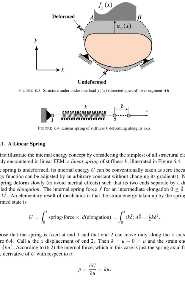
For distributed forces invariant in magnitude and direction, a spatial integration process is necessary to obtain P. These forces may include line loads, surface loads or volume loads (body forces). For example, consider the structure of Figure 6.3, on which a dead line load fy(x) acts in the y

direction along segment A B of the x axis. Then

P =

xB

xA

fy(x)uy(x)d x, (6.21)

where uy(x)is the y-displacement component of points on segment ( A,B). A similar technique

can be used for volume (body) forces as illustrated in Exercise 6.1.

Remark 6.2. Substantial mathematical complications arise if some forces are functions of the displacements. For example, in slender structures under aerodynamic pressure loads the change of direction of the forces as the structure deflects may have to be considered in the stability analysis. These so-called “follower” forces, which introduce force B.C. nonlinearities, are considered later in the course. Suffices to say here that no loads potential W generally exist in such cases, whence the system is nonconservative.

§6.5. Internal Energy Functions

The internal energy U is the recoverable mechanical work “stored” in the material of the structure by virtue of its elastic deformation. In the continuum mechanics models introduced in Chapters ? and following, that work is expressed in terms of strains and stresses and integrated over the body volume. In that context U is is called the strain energy. Note that only flexible bodies can store strain energy; a rigid body cannot. The examples that follow used only elastic springs, for which the continuum mechanics approach is unnecessary.

;; ;; ;; ;; Undeformed Deformed

_A

_B

x

y

f (x)

u (x)

Figure 6.3. Structure under under line load f_y(x)(directed upward) over segment A B.

; ; ; k δ x 2 1

Figure 6.4. Linear spring of stiffness k deforming along its axis.

§6.5.1. A Linear Spring

We first illustrate the internal energy concept by considering the simplest of all structural elements already encountered in linear FEM: a linear spring of stiffness k, illustrated in Figure 6.4.

If the spring is undeformed, its internal energy U can be conventionally taken as zero (because an energy function can be adjusted by an arbitrary constant without changing its gradients). Now let the spring deform slowly (to avoid inertial effects) such that its two ends separate by a distance

δ called the elongation. The internal spring force f for an intermediate elongation 0¯ ≤ ¯δ ≤ δ is ¯

f = kδ¯. An elementary result of mechanics is that the strain energy taken up by the spring in its deformed state is U = _δ 0 spring-force× d(elongation)= _δ 0 (kδ)¯ dδ¯ = ₂1kδ2. (6.22) Suppose that the spring is fixed at end 1 and that end 2 can move only along the x axis, as in Figure 6.4. Call u the x displacement of end 2. Then δ = u −0 = u and the strain energy is U = 1₂ku2. According to (6.2) the internal force, which in this case is just the spring axial force p, is the derivative of U with respect to u:

p = ∂U

∂u =ku. (6.23)

§6.5 INTERNAL ENERGY FUNCTIONS x y k Deformed Undeformed 1 1 1(x ,y ) 2 2 2(x ,y ) u u u u x1 y1 y2 x2

Figure 6.5. Linear spring of stiffness k displacing on the x,y plane.

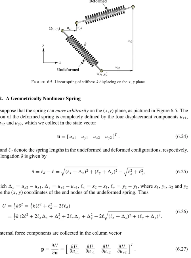
§6.5.2. A Geometrically Nonlinear Spring

Now suppose that the spring can move arbitrarily on the (x,y) plane, as pictured in Figure 6.5. The position of the deformed spring is completely defined by the four displacement components ux1, uy1, ux2 and uy2, which we collect in the state vector

u=[ ux1 uy1 ux2 uy2]T . (6.24)

Letandddenote the spring lengths in the undeformed and deformed configurations, respectively.

The elongationδis given by

δ =d −= (x+x)2+(y+y)2− 2 x +2y, (6.25)

in whichx = ux2−ux1,y = uy2−uy1, x = x2 −x1, y = y2− y1, where x1, y1, x2 and y2 denote the (x,y) coordinates of the end nodes of the undeformed spring. Thus

U = 1₂kδ2 = 1₂k(2+2_d −2d) = 1 2k(2 2₊₂ xx +2x +2yy+2y−2 (x +x)2+(y+y)2. (6.26)

The internal force components are collected in the column vector

p= ∂U ∂u = _∂ U ∂ux1 ∂U ∂uy1 ∂U ∂ux2 ∂U ∂uy2 T . (6.27)

The actual expressions of the components in (6.27) which are nonlinear functions of the displace-ments, are worked out in Exercise 6.2.

The important points that emerge from this example are:

1. The internal forces are nonlinear functions of the displacements, al-though the spring itself remains constitutively linear. This nonlinearity comes in as a result of geometric effects, and is thus properly called geometric nonlinearity.

2. The effect of geometric nonlinearities can be traced to the change in direction of the spring. Because if the spring stretches along its original axis the internal force remains linear in the displacements. This change of direction is measured by rotations.

Even for this simple case the exact nonlinear equations are quite nasty, involving irrational functions of the displacements. The second property, however, shows that approximations to the exact nonlinear equations may be made when the change in direction is “small” in some sense. This feature is illustrated in Exercise 6.3.

g

A

B

k

k

B'

A

B

C

C'

_θ

Figure 6.6. Inverted planar pendulum propped by extensional spring.

§6.5.3. A Spring-Propped Inverted Pendulum

This example illustrates the derivation of residual and incremental equations directly from energy for an angular (rotational) DOF. Figure 6.6 shows an inverted planar pendulum propped by an extensional spring, with the properties defined in the Figure. The pendulum is in a gravity field g acting as shown. There is only one state DOF: the tilt angleθ taken as positive CW. The system exhibits both geometric and force BC nonlinearities, the former because of finite rotations and the latter since the external force depends on that rotation). The geometric treatment is exact.

Internal and external energies are assumed to vanish atθ =0. If the pendulum is displaced by+θ from the vertical, the spring elongates byδ = L sinθ. Consequently the internal (stored) energy is U = 1₂ kδ2 = 1₂ k L2 sin2θ. The external work potential is W =λm g L(1−cosθ). This is+if

§6.6 *WORK DERIVATIVES λ K K K =1−λ θ (rad) θ (rad) p s s

(a)

(b)

Figure 6.7. Propped inverted pendulum of Figure 6.6: (a) response diagramλvs.

θfor m=k =L=g=1, showing primary(p) and secondary (s) equilibrium paths; (b) Tangent stiffness K for the equilibrium paths shown in (a).

the pendulum tilts in any direction, since if so the mass moves down and does positive work along the gravity field. Thus

=U −W = 1₂ k L2 sin2θ −λm g L(1−cosθ). (6.28) Differentiating once we get the residual force:

r = ∂

∂θ =k L

2

sinθ cosθ −λm g L sinθ, (6.29) Note that the system is non-separable because the RHS depends on both control λ and state θ.6 The equilibrium paths are given by the solutions of r = 0. These are θ = 0, λ = any and

λ = (k L)/(g m) cosθ for the primary and secondary path, respectively. These are plotted in Figure 6.7(a) over the rangeθ ∈ [−π, π] for the data k = L =m = g=1.

Differentiating once more gives the first-order rate equation Kθ˙=qλ˙ in which K = ∂r

∂θ = L(k L cos 2θ−λg m cosθ), q = − ∂r

∂λ =m g L sinθ. (6.30)

The value of K at both equilibrium paths is plotted in 6.7(b), also over the range θ ∈ [−π, π] for the data k = L = m = g = 1. Since K depends on bothλand θ, a 3D plot would be more arropriate. Further analysis of these results is relegated to an Exercise.

§6.5.4. Internal Energy Additivity Property

If the structure consists of m linear springs, each of which absorbs an internal energy Uk, the total

internal energy is the sum of the individual spring energies:

U =U1+U2 + . . . +Um. (6.31)

This additivity property is of course general because energies are scalar quantities. It applies to arbitrary structures decomposed into structural components such as finite elements. Furthermore, (6.31) is not affected by whether the structure is linear or nonlinear.

The last property (nonlinearity does not affect additivity) explains why FEM equations should be derived from energy functions if such functions exist, as already noted in §6.3.1.

§

6.6. *Work Derivatives

We collect here selected results connected to derivatives of the total potential energy (TPE). These results are of interest in sections dealing with solution methods.

§6.6.1. *Work Taylor Series

Consider the TPE evaluated at a state-control pair u, λthat is not necessarily an equilibrium point. We are interested in expressing the the TPE change when u and λare modified by small variations d and η, respectively. That is conveniently expressed by expanding in Taylor series. Retaining only the linear and quadratic terms of the series we have

d (u, λ)= (u+d, λ+η)− (u, λ)=[ d η] _r +1 2 [ d η] T K −q −qT _ϒ d η . (6.32) Here K and q have been previously defined, whereas

= ∂

∂λ, ϒ = ∂2

∂λ2 . (6.33)

Only W contributes toandϒ since U does not depends onλ. If the loading is proportional, W =λqT_u

and

=qTu, ϒ =0. (6.34)

§6.6.2. *Work Hessians and Dual Forms

For a conservative system the stiffness matrix and incremental load vector appear naturally as components of the following matrix of second derivatives:

  ∂ 2 ∂u∂u ∂ 2 ∂u∂λ ∂2 ∂λ∂u T ∂2 ∂λ∂λ  ₌ K −q −qT _ϒ (6.35) in whichϒ =∂2 _/∂λ2_{was introduced in (6.33). This symmetric matrix is called the augmented Hessian of}

. Note also that ∂q ∂u = ∂(−∂r/∂λ) ∂u = − ∂3 ∂u∂λ∂u = − ∂ ∂λ ∂2 ∂u∂u = − ∂K ∂λ = −Kλ, (6.36) is a symmetric matrix.

The complementary energy function ∗ may be defined from the dual Legendre transformation (see e.g., Chapter 2.5 of Sewell’s book [688]) as

+ ∗_=u

i

∂ ∂ui

=uTr=rTu. (6.37) This gives ∗(r, λ)=rT_{u− with u eliminated from r(u, λ)=0, so now the residual forces are the active}

variables. Obviously u= ∂ ∗ ∂r , or ui = ∂ ∗ ∂ri . (6.38)

The matrix of second derivatives of ∗is

  ∂ 2 ∗ ∂r∂r ∂ 2 ∗ ∂r∂λ ∂2 ∗ ∂λ∂r T ∂2 ∗ ∂λ∂λ  ₌ F v vT _ϒ∗ . (6.39)

§6.6 *WORK DERIVATIVES

These are linked to the quantities that appear in (6.35) by the matrix relations

F=K−1, v=K−1q=Fq, ϒ∗=qTK−1q−ϒ. (6.40) The converse relations are

K=F−1, q=Kv, ϒ =vTKv−ϒ∗. (6.41) The tangent flexibility matrix F=K−1(the Hessian of ∗) is now symmetric. Note also that

∂u ∂r = ∂3 ∗ ∂r∂λ∂r = ∂ ∂λ ∂2 ∗ ∂r∂r = ∂F ∂λ =Fλ, (6.42) is a symmetric matrix.

Remark 6.3. The following matrix appears (as amplification matrix) in the study of the stability of incremental methods:

A= ∂v ∂u = ∂(Fq) ∂u = ∂F ∂uq+F ∂q ∂u = ∂F ∂rKq+F ∂K ∂λ. (6.43)

Although A is unsymmetric, under some general conditions it has real eigenvalues. To show that we express A as the product of two symmetric matrices:

A= ∂v ∂u = ∂v ∂r ∂r ∂u = ∂F ∂λK=FλK, (6.44)

where the relation (6.42) has been used. If F_λis nonsingular, the eigensystem Axi = µixi can be transformed to the

generalized symmetric eigenproblem

Kxi =µiF_λ−1xi. (6.45)

If K is positive definite this system has nonzero real rootsµi. If Fλis singular but K positive definite, consideration of the

alternative eigensystem

F_λy_i =µiK−1yi =µiFyi, (6.46)

shows that such a singularity contributes only zero roots.

Remark 6.4. Another quantity that appears in the analysis of incremental methods is the vector

v= ∂v ∂λ = ∂v ∂u ∂u ∂λ=Av=FλKv=Fλq. (6.47)

Remark 6.5. Two other Legendre transforms may be constructed: X(,u)and Y(,r), in which=∂ /∂λ(a generalized displacement ifλis a load multiplier) is the active variable and either u or r take the role of passive variables. X and Y together with and K form a closed chain of Legendre transformations. The functions X and Y are, however, of limited interest in the present context.

§6.6.3. *Work Increments

Here we expand the above material a bit further, considering increments of u andλthat are not necessarily small; however, the pair(u, λ)is assumed to be at an equilibrium solution. We continue to assume that r is derivable from the potential = U −W . For questions such as positive path traversal it is interesting to

obtain an expression of the energy increment on passing from an equilibrium position(u, λ)to a neighboring configuration(u+u, λ+λ)

= (u+u, λ+λ)− (u, λ), (6.48) along an equilibrium path. First we note that adding an arbitrary function ofλto

does not change the equilibrium equations or rate forms. To second order in the increments we get =rTu+ λ+1 2u T_Ku−qT_uλ+ 1 2ϒ(λ) 2_{, (6.50)} But we can always adjust F(λ)in (6.49) so that=ϒ =0. Furthermore at an equilibrium position r=0,

and along the equilibrium pathu=K−1qλ=vλ. Substituting we find for the energy increment =U−W = ₂1qTv(λ)2−qTv(λ)2 = −1₂qTv(λ)2. (6.51) This formula displays the important function of the dot product qT_{v in the energy increment. By extension}

we may call

W =qTv(λ)2 (6.52)

the external work increment even if r does not derive from a potential. To fix the ideas assume that r derives from a quadratic potential

= 1 2u

T_Ku−qT_{uλ+Cλ+D, (6.53)}

where C and D are arbitrary constants. Then the increment from an equilibrium position(u, λ) that satisfies the linear relation Ku=qT_{λ, to an arbitrary configuration(u+u, λ+λ)is}

=uT(Ku−qTλ)+λ(qTu−C)= −λ(qTu−C)= −(qTvλ−C)λ. (6.54) Since C is arbitrary, chose it so that∂ /∂λ= −qT_{u+C=0. Then}

= −qTv(1₂λ2). (6.55)

Notes and Bibliography

Most of the material covered here is available in the literature, with the exception of that in §6.6. For a brief summary of the energy principles of mechanics, see the Wikipedia article at

https://en.wikipedia.org/wiki/Energy principles in structural mechanics

Exercises Homework Exercises for Chapter 6

Conservative Systems

Note: the use of a symbolic algebra package, such as Mathematica, is recommended for Exercises 6.3 and 6.4 to avoid tedious algebra and generate plots quickly. (There could be a gain from hours to minutes).

EXERCISE 6.1 [A:15] A body of volume V and densityρis in an uniform gravity field g acting along the −z axis. The body displaces to another position defined by the small-displacement field u(x,y,z). Find the expression of the load potential P as an integral over the body if the change in shape of the body is negligible.

EXERCISE 6.2 [A:20] Work out the detailed expression of the internal forces for (6.27). Then extend this relation to the three-dimensional case in which the ends of the spring move by ux1, uy1, uz1, ux2, uy2, uz2in

the x,y,z space.

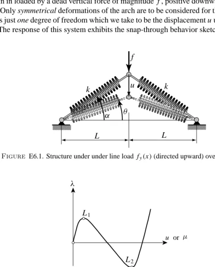
EXERCISE 6.3 [A+N/C:30] Consider the shallow arch model shown in Figure E6.1. This consists of two identical linear springs of axial stiffness k pinned to each other and to unmoving pinned supports as shown. The springs are assumed able to resist both tensile and compressive forces. The distance between the supports is 2L. The undeformed springs form an angleαwith the horizontal axis.

The central pin in loaded by a dead vertical force of magnitude f , positive downwards, which is parametrized as f =λk L. Only symmetrical deformations of the arch are to be considered for this Exercise. Consequently

the system has just one degree of freedom which we take to be the displacement u under the load, also positive downwards. The response of this system exhibits the snap-through behavior sketched in Figure E6.2.

;; ;; u f α θ k k L L

Figure E6.1. Structure under under line load f_y(x)(directed upward) over segment A B.

L1

L2

λ

u or µ

(a) Show that the internal energy U and load potential P of the two-spring system are given by U =k L2 1 cosα − 1 cosθ 2 , P = f u, (E6.1)

whereθ is the angle shown in Figure E6.1, which is linked to u by the relation tanθ+u/L =tanα. (b) Derive the exact equilibrium equation

r(u, λ)= ∂

∂u =0, (E6.2)

in which =U−P is the total potential energy, andλ= f/(k L)is the dimensionless state parameter. For convenience rewrite this as

r(µ, λ)=0, (E6.3)

in terms of the dimensionless state parameter

µ= u

L tanα. (E6.4)

(c) Derive the exact equation for the limit load parameters ∂λ(µ) ∂µ µ=µL,λ=λL =0. (E6.5) (Hint: the exact equation in terms of the angular coordinateθis cos3θ

L =cosα). Solve this trigonometric

equation7 _{for the limit-load parametersλ}

L1 andλL2 and the dimensionless displacementsµL1andµL2

at those points assuming thatα =30◦.

(d) If the arch initially is and remains sufficiently “shallow” throughout its snap-through behavior, we may make the small-angle approximations,

cosα≈1−1 2α

2_{, cosθ ≈1−}1 2θ

2_{, sinα≈tanα≈α, sinθ ≈tanθ ≈θ. (E6.6)} Recast the energy, equilibrium equations, and limit load equations in terms of these approximations, obtaining U as a quartic polynomial inθ, r as a cubic polynomial inθ, etc, then replace in terms ofµ. As a check, the residual equation in terms ofλandµshould be given by (4.16). Calculate the limit load parametersλL1 andλL2, and the dimensionless displacements µL1 andµL2 at those loads. Verify that

these displacements correspond to the anglesθL = ±α/

√ 3.

(e) Draw the control-state response curves r(µ, λ) = 0,derived using the exact nonlinear equations and those from the small-angle approximations on theλ, µplane (as in the sketch of Figure E6.2, going up toµ≈2.5) forα=30◦.

EXERCISE 6.4 [A+N:15] Derive the current stiffness parameterκ defined in Equations (5.17) and (5.18) for the approximate (small-angle) model of the two-spring arch of Exercise ?. Plot the variation ofκ(µ)asµ varies from 0 toµL1at the first limit point, withµalong the horizontal axis. Doesκvanish at the limit point?

EXERCISE 6.5 [A+N:15] Study the regions of stability and instability for the propped inverted pendulum problem of §6.5.3, as function ofλ,θand the data. Over the control-state plane (λ,θ), for k=L =m=g=1 draw the curve K =0 that separates stable and unstable regions while ignoring the equilibrium condition.