Ga¨
elle Chagny
To cite this version:
Ga¨elle Chagny. Adaptive warped kernel estimators. MAP5 2012-26. 2014. <hal-00715184v4>
HAL Id: hal-00715184
https://hal.archives-ouvertes.fr/hal-00715184v4
Submitted on 31 Jan 2014
HAL is a multi-disciplinary open access archive for the deposit and dissemination of sci-entific research documents, whether they are pub-lished or not. The documents may come from teaching and research institutions in France or abroad, or from public or private research centers.
L’archive ouverte pluridisciplinaire HAL, est destin´ee au d´epˆot et `a la diffusion de documents scientifiques de niveau recherche, publi´es ou non, ´emanant des ´etablissements d’enseignement et de recherche fran¸cais ou ´etrangers, des laboratoires publics ou priv´es.
ADAPTIVE WARPED KERNEL ESTIMATORS
GAËLLE CHAGNYA ∗
Abstract. In this work, we develop a method of adaptive nonparametric estimation, based on "warped" kernels. The aim is to estimate a real-valued functionsfrom a sample of random couples
(X, Y). We deal with transformed data(Φ(X), Y), withΦa one-to-one function, to build a collec-tion of kernel estimators. The data-driven bandwidth seleccollec-tion is done with a method inspired by Goldenshluger and Lepski (2011). The method permits to handle various problems such as addi-tive and multiplicaaddi-tive regression, conditional density estimation, hazard rate estimation based on randomly right censored data, and cumulative distribution function estimation from current-status data. The interest is threefold. First, the squared-bias/variance trade-o is automatically realized. Next, non-asymptotic risk bounds are derived. Last, the estimator is easily computed thanks to its simple expression: a short simulation study is presented.
Keywords: Adaptive estimator. Censored data. Bandwidth selection. Nonparametric estimation. Regression. Warped kernel.
AMS Subject Classication 2010: 62G05; 62G08; 62N02. 1. Introduction
Let (X, Y) be a couple of real random variables, and (Xi, Yi)i=1,...,n an i.i.d. sample drawn as
(X, Y). The main goal of nonparametric estimation is to recover an unknown function s, linked
with (X, Y), such as the regression function, from the data. Among the huge variety of methods that have been investigated, the use of transformed data (FX(Xi), Yi), with FX the cumulative
distribution function (c.d.f.) ofX, has received attention in the past decades. In this context or with
similar tools, both kernel and projection estimators have been studied in random design regression estimation (Yang 1981, Stute 1984, Kerkyacharian and Picard 2004, Akritas 2005, Pham Ngoc 2009, Kulik and Raimondo 2009, Mammen et al. 2012, Chagny 2013a), conditional density or c.d.f estimation (Stute 1986, Mehra et al. 2000, Chagny 2013c), for the white noise model (Chesneau 2007) or to deal with dependent data (Chesneau and Willer 2012). However, to our knowledge, few papers focus on the problem of adaptivity of such "warped estimators". The aim of the present work is twofold: rst, we want to show that a warping kernel device can be applied to various estimation problems, including survival analysis models (see examples below). Secondly, we address the problem of bandwidth selection, with the intention of providing an adaptive "warped" estimator, which satises nonasymptotic risk bounds.
The basic idea, which motivates the study of warped kernel estimators introduced by Yang (1981), can be rst explained in the classical regression framework. Here, the target function is the conditional expectation,s:x7→E[Y|X =x]i.e.
(1) s(x) = 1
fX(x)
∫
Ryf(X,Y)(x, y)dy,
∗Corresponding author. Email: [email protected]
ALaboratoire MAP5 (UMR CNRS 8145), Université Paris Descartes, and LMRS (UMR CNRS 6085), Université de
Rouen, France.
when a density f(X,Y) for the couple (X, Y) exists, and where fX is the marginal density of the
design X. Historical kernel methods were initiated by Nadaraya (1964) and Watson (1964). The
famous estimator named after them is built as the ratio of a kernel estimator of the productsfX
divided by a kernel estimator of the densityfX:
˜ sN W :x7→ 1 n ∑n i=1YiKh(x−Xi) 1 n ∑n i=1Kh(x−Xi) ,
where Kh : x 7→ K(x/h)/h, for h > 0, and K : R → R such that
∫
RK(x)dx = 1. Adaptive
estimation then requires the automatic selection of the bandwidth h, and the ratio form of the
estimate suggests that two such parameters should be selected: one for the numerator, and one for the denominator. From the theoretical point of view, there is no reason to choose the same. Nevertheless, nonasymptotic results such as oracle-inequality are dicult to derive for an estimator dened with two dierent data-driven smoothing parameters. See Penskaya (1995) for a thorough study of the ratio-form estimators. Moreover, when the design X is very irregular (for example
when a "hole" occurs in the data), a ratio may lead to instability (see Pham Ngoc 2009). The warped kernel estimators introduced by Yang (1981) and Stute (1984) avoid the ratio-form. Indeed denote byFˆn the empirical c.d.f. of theXi's and let
(2) ˆsh = 1 n n ∑ i=1 YiKh(FX(x)−FX(Xi)), or ˆsh = 1 n n ∑ i=1 YiKh ( ˆ Fn(x)−Fˆn(Xi) ) ,
depending on whether the c.d.f. FX is known or not. The following equality (see (8)) holds:
E[Y Kh(u−FX(X))] =Kh⋆(s◦FX−1)(u),
where⋆ is the convolution product and ◦ is the composition symbol. Thus, the rst estimator of
(2) can be viewed as sˆh = s\◦FX−1◦FX. The main advantage is that its expression involves one
bandwidthh only.
In this paper, we generalize the warping strategy to various functional estimation problems: as a rst extension of (1), we propose to recover functionssof the form
(3) s(x) = 1
ϕ(x)
∫
θ(y)f(X,Y)(x, y)dy,
for θ : R → R, and ϕ : R → R+\{0}. In this case, the warping device brings into play the transformation (Φ(X), Y) of the data, with Φ′ = ϕ. The form (3) covers the additive regression
model described above, by setting Φ = FX, and θ(y) = y. But it also permits to deal with the
simplied heteroskedastic model Y = √s(X)ε, where ε is an unobserved noise, centered, with
variance equals to 1. In this case,Φ =FX, andθ(y) =y2.
In several examples however, the couple(X, Y)does not admit a density, butXadmits a marginal
density. Then (3) can be extended and the target functionstakes the form:
(4) s(x) = fX(x)
ϕ(x) E[θ(Y)|X=x].
This allows to handle two classical settings in survival analysis: the interval censoring case 1, and right censored data. In the interval censoring model, case 1, the target function iss(x) =P(Z ≤x), whereZis a survival time, which is not observed, and we only know a current status at the observed
timeX of examination. We also know Y =1Z≤X, which indicates whether Z occurs before X or
not. We refer to Jewell and van der Laan (2004) for a review of the estimation methods in this setting (see also van de Geer 1993 for maximum likelihood estimation), and more recently to Ma and Kosorok (2006), Brunel and Comte (2009) or Plancade (2013) for investigations including adaptivity. In right-censored data, the function of interest at time x is the hazard rate function, that is the
risk of death at time x, given that the patient is alive until x. This model has been studied by
Tanner and Wong (1983), Müller and Wang (1994) and Patil (1993), among all. Adaptive results are available for projection-type estimators (see Brunel and Comte 2005, 2008, Reynaud-Bouret 2006 or Akakpo and Durot 2010), but to our knowledge not for kernel estimators.
The paper is organized as follows. We present in Section 2 the estimation method, detail the examples illustrating the relevance of the introduction of a general target function s dened by
(4). We also study the global risk of the warped kernel estimators with xed bandwidths. Section 3 is devoted to adaptive estimation: we dene a data-driven choice of the bandwidth, inspired by Goldenshluger and Lepski (2011) which allows to derive nonasymptotic results for the adaptive estimators. Oracle-type inequalities are provided for the M.I.S.E., and convergence rates are deduced under regularity assumptions. Sections 2 and 3 both deal with the case of known deformation Φ and with the case of an estimated deformation. In Section 4, the method is illustrated through numerical simulations. Proofs are gathered in Section 5. The supplementary material Chagny (2013b) is available for further details about technical computations.
2. Estimation method
2.1. Warped kernel strategy. Consider a sample (Xi, Yi)i=1,...,n of i.i.d. random couples with
values inA×B, whereAis an open interval ofRandB a Borel subset ofR. We assume thatXi has
a marginal densityfX and we aim at recovering a functions:A→Rlinked with the distribution of
(Xi, Yi). To estimates, we replace the explanatory variableXi byΦ(Xi), whereΦ :A→Φ(A)⊂R
is one-to-one and absolutely continuous. The data(Φ(Xi), Yi)i=1,...,n are called the warped sample
with deformation function Φ. The sets A, B,Φ(A) are supposed to be given. The target function can be written as:
(5) s(x) =g◦Φ(x) =g(Φ(x)), withg : Φ(A)→R.
We rst estimate the auxiliary functiong=s◦Φ−1withΦ−1the inverse function ofΦ. In the general case, Φ is unknown and we must estimate it also. LetK be a function such that ∫RK(u)du = 1 and setKh:u7→K(u/h)/h, forh >0. We dene, foru∈Φ(A),
(6) gˆh(u) = 1 n n ∑ i=1 θ(Yi)Kh ( u−Φˆn(Xi) ) ,
whereθ:R→Ris a given function, Φˆn is an empirical counterpart for Φ, and forx∈A
(7) sˆh(x) = ˆgh◦Φˆn(x) = 1 n n ∑ i=1 θ(Yi)Kh ( ˆ Φn(x)−Φˆn(Xi) ) .
The following equality is the cornerstone of the method and justies the introduction of (6). If θ
satisesE|θ(Y)Kh(u−Φ(X)|<∞, for allu∈Φ(A),
(8) E[θ(Y)Kh(u−Φ(X)] =Kh⋆
(
g1Φ(A))(u) :=gh(u),
where⋆ is the convolution product. It shows thatgˆh is an empirical version of gh and thus sˆh in
(7) suits well to estimates. Let us give examples covered by the above framework.
Example 1 (standard random design regression with additive error term): we observe (Xi, Yi)withYi =s(Xi) +εi,(εi)i=1,...,nis independent of(Xi)i=1,...,n,E[ε2i]<∞andE[εi] = 0. We
choose Φ(x) =FX(x), the cumulative distribution function (c.d.f. in the sequel) of X and assume
Example 2 (Heteroskedastic model): Yi = σ(Xi)εi, (εi)i=1,...,n independent of (Xi)i=1,...,n,
E[ε2i] = 1,E[εi] = 0,Φ(x) =FX(x), withΦ :A→Φ(A)invertible. Heres(x) =σ2(x) =E[Yi2|Xi =
x].
Example 3 (Interval censoring, Case 1): the observation is (Xi, Yi) where Yi = 1Zi≤Xi,
Zi, Xi ≥ 0 are independent event occurence times, Yi indicates whether Zi (the time of interest)
occurs before Xi (the so-called examination time) or not and Zi is not observed. The target
function iss(x) =P(Zi ≤x) =E[Yi|Xi =x]. We choose Φ =FX.
Example 4 (Hazard rate estimation from right censored-data): the observation isXi =Zi∧
Ci,Yi =1Zi≤Ci, whereZi andCiare not observed and independent,Zi≥0is a lifetime andCi ≥0 is a censoring time. The functionsof interest is the hazard rate functions(x) =fZ(x)/(1−FZ(x)),
wherefZ (resp. FZ) is the density (resp. the c.d.f.) ofZ. This function satises
(9) s(x) = fX(x) 1−FX(x)E
[Y|X=x].
In this case, we assumeFX(x)<1 for all x≥0, and take Φ(x) =
∫x
0(1−FX(t))dt.
We now dene the estimator Φˆ of the warping function Φ. Instead of estimating Φ with the whole sample (Xi)i=1,...,n, we assume that another sample (X−i)i=1,...,n, independent of the Xi's,
but distributed like them, is available. Thus, we set ˆ Φn(x) = {ˆ Fn(x)(Examples 1-3), ∫x 0 ( 1−Fˆn(t) ) dt(Example 4) where Fˆn(x) = n1 ∑n i=11X−i≤x.
The introduction of the second sample of variableX is an artefact of the theory: it only allows to
avoid dependency problems in the proof of the results, which are technical and cumbersome enough (see the supplementary material Chagny 2013b). This trick is also standard in others studies of warped methods (see Kerkyacharian and Picard 2004 or Kulik and Raimondo 2009 e.g.). Using a single sample would have required totally dierent statistic and probabilistic tools. However, we have obviously used only one sample to compute the estimator in the simulation study, see Section 4 (otherwise the comparison with other methods would not have been fair).
Hereafter, we also denote by ˜gh the pseudo-estimators dened by choosing Φ = Φˆ in (6). We
coherently sets˜h= ˜gh◦Φ. They can be used whenΦis known. The theoretical results are the same
fors˜h andsˆh, up to further technicalities due to the plug-in of an empirical version forΦ. The paper
mainly focuses on the proofs of the results fors˜since they are representative of the statistical and probabilistic tools which are required. Complete proofs are available in the supplementary material Chagny (2013b).
2.2. Risk of the xed bandwidth estimator. In this section, we study the global properties of sˆh as an estimate of s on A, with a xed bandwidth h. The quadratic risk weighted by the
derivativeϕ of the warping functionΦ is the natural criterion in our setting. Let us introduce, for a measurable functionton A,
(10) ∥t∥2ϕ=
∫
A
t2(x)ϕ(x)dx,
and denote byL2(A, ϕ) the space of functionstfor which the quantity (10) exists and is nite. We
also use the corresponding scalar product⟨., .⟩ϕ. Fort1, t2 belonging to L2(A, ϕ), we have
where ∥t1∥2L2(Φ(A)) = ∫
Φ(A)t 2
1(x)dx and ⟨., .⟩Φ(A) denotes the usual scalar product on L2(Φ(A)). Therefore,
∥s˜h−s∥2ϕ=∥g˜h−g∥2L2(Φ(A)).
WhenK belongs toL2(R) and E[θ2(Y1)]<∞, the following bias-variance decomposition of the risk holds (recall that gh is dened in (8)),
(11) E[∥s˜h−s∥2ϕ ] ≤ ∥g−gh∥2L2(Φ(A))+ 1 nhE [ θ2(Y1) ] ∥K∥2L2(R).
This inequality holds ifs∈L2(A, ϕ), a property which is satised if sis bounded on A. This is the
case for Examples 1-3, as ϕ= fX. In Example 4, we can check that s∈ L2(A, ϕ) for all classical
distributions forC and Z used in survival analysis (such as exponential, Weibull, Gamma...). The
general condition to be checked in this example is∫AfX2(x)/(1−FX(x))dx <∞.
The challenge in the general case comes from the plug-in of the empirical Φˆn. Though natural, it necessitates lengthy and cumbersome technicalities. This explains why it is not often considered in the literature of warped estimators (see e.g. Pham Ngoc 2009 or Chesneau 2007). The following assumptions are required.
(H1') The functionsis continuously derivable on A.
(H2') The kernelK is twice continuously derivable, with bounded derivativesK′ andK′′ on R.
(H3') The set A can be writtenA= (0, τ) with nite τ >0, in Example 4.
Assumption (H1') is somehow restrictive but required for integration by parts (see Section C.3. in Chagny (2013b)). Assumption (H2') permits to use Taylor formulas to deal with the dierence
Kh(u−Φˆn(Xi))−Kh(u−Φ(Xi)). This is not a problem as we choose the kernel in practice. We
also add (H3'), which is needed to control the dierence Φˆn−Φˆ in Example 4 (see Section B. in Chagny (2013b)). Thanks to technical computations, we obtain the analogous of (11) forsˆh, under
mild assumptions. A sketch of the proof is given in Section 5.2. The details are provided in Chagny (2013b).
Proposition 1. Assume (H1'), and (H2'), and also (H3') for Example 4. If moreover h≥Cn−1/5
(C a purely numerical constant), there exists c >0 such that (12) E[∥sˆh−s∥2ϕ ] ≤5∥g−gh∥2L2(Φ(A))+ c nh. 3. Adaptive estimation
As usual, we must choose a bandwidthhwhich realizes the best compromise between the
squared-bias and the variance terms (see (11) and (12)). The choice should be data-driven. For this, we use a method described in Goldenshluger and Lepski (2011), and show that this leads to oracle-type inequalities and adaptive optimal estimators (in the sense of Goldenshluger and Lepski 2011). We begin with the case of known warping functionΦ, which permits to develop the theoretical tools in a simpler way and to derive the results with few assumptions and short proofs.
3.1. Case of known Φ.
3.1.1. Data-driven choice of the bandwidth. We consider the collection (˜sh)h∈Hn, where Hn is a
nite collection of bandwidths, with cardinality depending on n and properties precised below
(Assumptions (H2)-(H3)). We introduce the auxiliary estimators, involving two kernels, ˜ sh,h′(x) = ˜gh,h′(Φ(x)) with g˜h,h′ =Kh′⋆ ( ˜ gh1Φ(A) ) .
For a numerical constantκ >0to be precised later on (see Section 4.1 below), we dene, forh∈ Hn,
(13) V(h) =κ ( 1 +∥K∥2L1(R) ) ∥K∥2L2(R)E [ θ2(Y1) ] 1 nh.
Next, we set (14) A(h) = max h′∈Hn { ∥s˜h,h′−˜sh′∥2ϕ−V(h′) } +,
which is an estimation of the squared-bias term (see Lemma 4). Note that∥s˜h,h′−˜sh′∥2ϕ=∥˜gh,h′−
˜
gh′∥2. Lastly, the adaptive estimator is dened in the following way:
(15) ˜s= ˜s˜h with h˜=argmin
h∈Hn
{A(h) +V(h)}.
The selected bandwidth ˜h is data-driven. In V(h), the expectation E[θ2(Y
1)] can be replaced by the corresponding empirical mean (see Brunel and Comte 2005, proof of Theorem 3.4 p.465). In Examples 3-4, it can be replaced by1, its upper-bound.
3.1.2. Results. We consider the following assumptions:
(H1) The functionsis bounded. Denote by ∥s∥L∞(A) its sup-norm. (H2) There existα0 >0 and a constantk0 ≥0such that
∑
h∈Hn 1
h ≤k0n
α0.
(H3) For allκ0 >0, there exists C0 >0, such that ∑ h∈Hn exp ( −κ0 h ) ≤C0.
(H4) The kernel K is of order l, i.e. for all j ∈ {1, . . . , l+ 1}, the function x 7→ xjK(x) is integrable, and for 1≤j≤l,∫RxjK(x)dx= 0.
Assumption (H1) is required to obtain Theorem 2 below. Nevertheless the value ∥s∥L∞(A) is not needed to compute the estimator (see (15)). This assumption holds in Example 3 (s ≤ 1 in this case), and in Example 4, for instance whenZ has exponential or Gamma distribution. Assumptions
(H2)-(H3) mean that the bandwidth collection should not be too large. For instance, the following classical collections satisfy these assumptions:
(1) Hn,1 = { k−1, k= 1, . . . , χ(n)}withα0 = 2,χ(n) =nor α0 = 1,χ(n) = √ n. (2) Hn,2 = { 2−k, k = 1, . . . ,[ln(n)/ln(2)]}, withα 0 = 1.
Assumption (H4) is required only to deduce convergence rate from the main nonasymptotic result. We need a moment assumption linked with (H2):
(H5) Withα0 given by (H2), there exists p >2α0, such that E[|θ(Y)−E[θ(Y)|X]|2+p]<∞. Ifθ is bounded, (H5) evidently holds. In Examples 1 and 2, (H5) is a moment assumption on the
noise which is usual in regression settings. It includes e.g. the case of Gaussian regression (when the noise ε is a Gaussian variable), under Assumption (H1). Notice also that the smaller α0, the
less restrictive the integrability constraintp on the noise moments.
We prove the following oracle-type inequality:
Theorem 2. We assume that (H1)-(H3) hold in Examples 1-4, and additionally that (H5) is fullled for Examples 1-2. Then there exist two constantsc1 >0 and c2>0, such that:
(16) E[∥s˜−s∥2ϕ ] ≤c1 min h∈Hn { ∥s−sh∥2ϕ+ E[θ2(Y1) ] ∥K∥2L2(R) nh } + c2 n,
with sh=gh◦Φand s˜dened by (15). The constant c1 only depends on ∥K∥L1(R).
The constant c2 depends on ∥s∥L∞(A), ∥K∥L1(R) and ∥K∥L2(R) in Examples 3-4, and also on the moment ofε and E[s2(X1)] for Examples 1-2. The adaptive estimator s˜automatically makes the
squared-bias/variance compromise. The selected bandwidth˜his performing as well as the unknown oracle:
h∗ :=arg min
h∈HnE
[∥s˜h−s∥2ϕ].
up to the multiplicative constantc1 and up to a remainding term of order 1/n, which is negligible. The interest of Inequality (16) is that it is nonasymptotic. Moreover, contrary to usual kernel estimation results, Assumption (H4) is not needed. This is one of the advantages of the bandwidth selection method. Inequality (16) proves that the estimators˜is optimal in the oracle sense.
To deduce convergence rates, smoothness classes must be considered to quantify the bias term. Dene the Hölder class with orderβ >0and constantL >0 by
H(β, L) =
{
t:R→R, t(⌊β⌋) exists,∀x, x′ ∈B, t(⌊β⌋)(x)−t(⌊β⌋)(x′)≤L|x−x′|β−⌊β⌋
}
,
where⌊β⌋ is the largest integer less thanβ. We also need the Nikol'skii class of functions:
N2(β, L) = { t:R→R, t(⌊β⌋) exists, ∀x∈R, ∫ R ( t(⌊β⌋)(x′+x)−t(⌊β⌋)(x′) )2 dx′ ≤L2|x|2β−2⌊β⌋ } We can now deduce from Theorem 2 the convergence rate of the risk, under regularity assumptions for the auxiliary functiong.
Corollary 1. Letg¯=g1ϕ(A) on R. Assume that
• g¯belongs to the Hölder class H(β, L), with ¯g(0) = ˜g(1) in Examples 1-3,
• g¯belongs to the Nikol'skii class N2(β, L) in Example 4.
Assume (H4) withl=⌊β⌋. Then, under the assumptions of Theorem 2,
(17) E[∥˜s−s∥2ϕ
]
≤Cn−2β+12β , where C is a constant which does not depend on nand β.
In Examples 1-3,Φ(A) = (0; 1)and the Hölder condition is enough. In Example 4,Φ(A) =R+ and we need the Nikol'skii condition. Both spaces are standard in kernel estimation, see e.g. Tsybakov (2009) and Goldenshluger and Lepski (2011).
We recover the classical optimal rates in nonparametric estimation. Note however that our regularity assumptions are set on g and not s, as long as we do not consider specic warped spaces dened
in Kerkyacharian and Picard (2004). The rate (17) is known to be optimal in the minimax sense for the estimation problems we consider (e.g., see Korostelëv and Tsybakov 1993 for regression estimation, Huber and MacGibbon 2004 for hazard rate, and Plancade 2013 for c.d.f. estimation with current-status data), if the two functions have the same regularity parameter.
Remark 1. We have strong conditions ongat the boundary of the support[0; 1], in Examples 1-3. This is nevertheless well-known in kernel estimation, which are rarely free of boundary eects. This also explains why we restrict the estimation interval for the simulation study, by using the quantiles of the observations Xi (see Section 4). Notice that we may apply recent methods which
provide boundary corrections in kernel estimation (see Karunamuni and Alberts 2005 and Bertin and Klutchniko 2011 for example), but this is beyond the scope of this paper. Moreover, the comparison against adaptive smoothing splines, which have no such problem of boundary already give good results in practice, see Section 4 below.
3.2. General case of unknownΦ. We use the plug-in device ofΦˆnin the denition of the
quanti-ties (13) and (14) to introduce a criterion like (15) which is fully data-driven in the general case of un-known warped function. To limit the technicalities, we focus on one of the following bandwidth col-lectionHn: Hn,1 ={k−1, k= 1, . . . ,[(n/ln(n))1/5]} or Hn,2 ={2−k, k= 1, . . . ,[ln(n)/(6 ln(2))]}.
The selection of an estimator in the collection(ˆsh)h∈Hn,l,l= 1,2, is done with (18) ˆh=arg min h∈Hn,l { b A(h) + 2Vb(h) } , with (19) Ab(h) = max h′∈Hn { ∥gˆh,h′−ˆgh′∥L22(Φ(A))−Vb(h′) } +,
andVb(h) =κ′ln2(n)/nh, where,κ′ is a purely numerical constant given by the proofs (see Chagny
2013b, Section D) and tuned in practice (see Remark 2). Finally, we dene sˆ = ˆsˆh ◦Φˆn. The
following result is the equivalent to Theorem 2.
Theorem 3. We assume that (H1), (H1')-(H2') hold in Examples 1-4, and additionally that (H5) is fullled for Examples 1-2 (withα0 = 1), and (H3') for Example 4. Then there exist two constants
c′1, c′2 >0, such that, for n large enough,
(20) E[∥sˆ−s∥2ϕ ] ≤c′1 min h∈Hn,l { ∥s−sh∥2ϕ+ ln2(n) nh } +c ′ 2 n,
with sh=gh◦Φ, and for l= 1,2.
The proof of Theorem 3, which follows the same scheme than the one of Theorem 2, is provided in the supplementary material Chagny (2013b). The values of the constants are specied in the proof. They depend on K and s, but neither on n, nor on the bandwidth h. The term Vb in the
denition (18) of the criterion deserves some comments. It can be compared to the penalty V
dened in the toy case of knownΦ in (13). The order of magnitude is not exactly the same: here, we have an extra-logarithmic factor. It is due to the substitution ofΦˆnto Φ, and plays a technical role in the proof but it gives what is usually called a nearly optimal bound. Note that it does not depend onE[θ2(Y1)], contrary to (13).
4. Illustration
To illustrate the procedure, we only focus on two of the four examples: the additive regression (Example 1), and the estimation of c.d.f. under interval censoring case I (Example 3). As we cannot reasonably pretend to compare our method with all the adaptive estimators of the literature, we choose to concentrate on the comparison with adaptive least-squares (LS in the sequel) estimators. 4.1. Implementation of the warped-kernel estimators. The theoretical study allows the choice of several kernels and bandwidth collections. For practical purpose, we consider the Gaussian kernel, K :x 7→e−x2/2/√2π, which satises Assumption (H4) with l = 1. It has the advantage of having simple convolution-products:
(21) ∀h, h′ >0, Kh⋆ Kh′ =K√h2+h′2.
The experiment is conducted with the dyadic collection Hn,2 dened above. The larger collection
Hn,1has also been tested: since it does not really improve the results but increases the computation time, we only keep the other collection. Besides, the simulations are performed in the case of unknownΦ. Therefore in Examples 1 and 3, the estimator is
ˆ s : x 7→ 1 n n ∑ i=1 θ(Yi)Kˆh( ˆFn(x)−Fˆn(Xi)),
with Fˆn the empirical c.d.f. of the Xi's. Then, the estimation procedure can be decomposed in some steps:
•ComputeVb(h)andAb(h)for eachh∈ Hn,1. ForVb(h), we setκ′ = 0.05in Example 1, andκ′ = 0.3
in Example 3 (see Remark 2 below). For Ab(h), thanks to (21), the auxiliary estimates are easily computed: sˆh,h′ = ˆs√h2+h′2. TheL2−norm is then approximated by a Riemann sum:
∥ˆgh,h′−gˆh′∥2L2(Φ(A))≈ 1 N N ∑ k=1 ( ˆ gh,h′(uk)−gˆh′(uk) )2 ,
whereN = 50, and(uk)k are grid points evenly distributed across(0; 1).
•Selectˆh such thatAb(h) + 2Vb(h)is minimum.
•Compute ˆshˆ.
Remark 2. The computation of the selection criterion (18) requires a value forκ′. A lower bound
for its theoretical value is provided by the proof: it is very pessimistic due to rough upper-bounds (for the sake of clarity), and obviously useless in practice, like in most model selection devices. We have carried out a large number of simulations to tune it, prior to the comparison with the other estimates. We have plotted the quadratic risk in function ofκ′ for various models and we have chosen
one of the rst values leading simultaneously to a reasonable risk and a reasonable complexity of the selected bandwidth. Such procedure is classical, and required whatever the chosen selection device (see e.g. Sansonnet 2013 for a similar tuning method in wavelet thresholding, or Chagny 2013a for details of tuning in model selection).
4.2. Example 1: additive regression. We compare the warped kernel method (WK) with the adaptive estimator studied in Baraud (2002). It is a projection estimator, developed in an or-thogonal basis of L2(A), and built with a penalized least-squares contrast. The experiment is carried out with the Matlab toolbox FY3P, written by Yves Rozenholc, and available on his web page http://www.math-info.univ-paris5.fr/∼rozen/YR/Softwares/Softwares.html. A regu-lar piecewise polynomial basis is used, with degrees chosen in an adaptive way. Since the kernel we choose has only one vanishing moment, the comparison is fair if we consider polynomials with degrees equal to or less than 1. We denote by LS1 the resulting estimator. However, as shown below, we will see that the warped-kernel generally outperforms the least-square, even if we use polynomials with degree at most 2 (LS2). We also experiment the Fourier basis for the least-squares estimator, but the results are not as good as the polynomial basis. Thus, we do not mention the values of the risks.
The procedure is applied for dierent regression functions, design and noise. The main goal is to illustrate the sensibility of the estimation to the underlying design distribution. Its inuence is explored through four distributions: two classical ones, U[0;1], the uniform distribution on the interval[0; 1], andN(0.5,0.01), a Gaussian distribution (with mean0.5and variance0.01); and two distributions which are more original (more irregular), γ(4,0.08), the Gamma distribution, with parameters4and0.08(0.08is the scale parameter), andBN a bimodal Gaussian distribution, with densityx7→c(exp(−200(x−0.05)2) + exp(−200(x−0.95)2)) (cis a constant adjusted to obtain a
density function).
We focus on the three following regression functions
s1 : x7→x(x−1)(x−0.6)
s2 : x7→ −exp(−200(x−0.1)2)−exp(−200(x−0.9)2) + 1
s3 : x7→cos(4πx) + exp(−x2)
The rst two functions satisfy the periodicity assumptions of Corollary 1, while we choose the functions3 to show that our procedure also leads to satisfactory results if the assumption does not hold. The choice of the functions2combined with the designBN leads to a data set which presents a "hole" (see Figure 2 (a)).
0.1 0.2 0.3 0.4 0.5 0.6 0.7 0.8 0.9 −0.5 0 0.5 1 1.5 2 0.1 0.2 0.3 0.4 0.5 0.6 0.7 0.8 0.9 −0.5 0 0.5 1 1.5 2 (a) (b) 0.1 0.2 0.3 0.4 0.5 0.6 0.7 0.8 0.9 −0.5 0 0.5 1 1.5 2 0.1 0.2 0.3 0.4 0.5 0.6 0.7 0.8 0.9 −0.5 0 0.5 1 1.5 2 (c) (d)
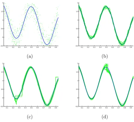
Figure 1. Estimation in Example 1, with true regression functions3, design distribution U(0;1), and n = 1000. (a) points: data(Xi, Yi)i, thick line: true functions3. (b)-(c)-(d) beams of 20 estimators built from i.i.d. sample (thin lines) and true function (thick line): warped kernel estimators (subplot (b)), least-squares estimator in piecewise polynomial bases with degree at most 1 (subplot (c)) or 2 (subplot (d)).
We also test the sensibility of the method to the noise distribution: contrary to the underlying design distribution, it does not seem to aect the results. Thus, we present the simulation study for a Gaussian centered noise, with variance σ2. The value of σ is chosen in such a way that the
signal-to-noise ratio (the ratio of the variance of the signal Var(s(X1))over the variance of the noise Var(ε1)) approximately equals 2.
Beams of estimators (WK, LS1, and LS2) are presented in Figures 1 and 2, with the generated data-sets and the function to estimate. Precisely, Figure 1 shows a regular case: all the methods estimate correctly the signal. Figure 2 depicts the case where a hole occurs in the design density: the estimator built with warped kernel behaves still correctly, even if the data are very inhomogeneous, while the estimator LS1, with which the comparison is fair, failed to detect the hole.
A study of the risk is reported in Tables 1 and 2, for the sample sizes n = 60,200,500 and 1000. The MISE is obtained by averaging the following approximations of the ISE values, for
j∈ {1, . . . , J = 200}, computed withJ sample replications:
ISEj = b−a N N ∑ k=1 (˜s(xk)−s(xk))2,
where s˜ stands for one of the estimators, b is the quantile of order 95% of the Xi and a is the
quantile of order5%. The(xk)k=1,...,N are the sample points falling in[a;b]. Tables 1 and 2 display
the values computed for our method WK, and for the estimators LS1 and/or LS2: for the regression functionss1 and s2 (Table 1), the warped-kernel strategy always leads to smaller risk values than
0 0.1 0.2 0.3 0.4 0.5 0.6 0.7 0.8 0.9 1 0 0.5 1 1.5 0 0.1 0.2 0.3 0.4 0.5 0.6 0.7 0.8 0.9 1 0 0.5 1 1.5 (a) (b) 0 0.1 0.2 0.3 0.4 0.5 0.6 0.7 0.8 0.9 1 0 0.5 1 1.5 0 0.1 0.2 0.3 0.4 0.5 0.6 0.7 0.8 0.9 1 0 0.5 1 1.5 (c) (d)
Figure 2. Estimation in Example 1, with true regression functions2, design distribution BN, andn= 1000. (a) points: data(Xi, Yi)i, thick line: true functions2. (b)-(c)-(d) beams of 20 estimators built from i.i.d. sample (thin lines) and true function (thick line): warped kernel estimators (subplot (b)), least-squares estimator in piecewise polynomial bases with degree at most 1 (subplot (c)) or 2 (subplot (d)).
LS1. Thus, we only mention the risks of the estimator LS2: even if the comparison is quite unfair (following the theoretical results, see the explanations above), the WK and the LS2 estimators are comparable in terms of performance and in 56% of the examples, the risks of the warped-kernel estimator are smaller than the ones of LS2 estimator. For the third function (Table 2), our method still outperforms the least-squares estimate in polynomial basis of degree at most 1, whatever the design distribution is. The comparison with least-squares in polynomial basis with degree at most 2 leads to mixed results even if the values for both estimators are in the same range. Our estimators still behaves correctly (compared to LS1, see also Figure 1), but not as well as for the rst two functions. Considering the denition of s3, the equality s3(a) =s3(b), required for the theoretical convergence rate does not hold, which may explain the result.
To conclude, if both methods LS2 and WK lead to comparable risks, it remains that our procedure have some advantages, compared to adaptive least-squares methods. First it is easier to implement, since it does not require any matrix inversion (compared to any LS strategy, see Baraud 2002). Then, keeping in mind that the comparison is fair when choosing piecewise polynomials with degree at most 1, the risk values are always smaller for the warped-kernel estimates, in the studied examples. Finally, we are able to recover a signal even with an irregular design, while the least-squares methods fail in that case.
4.3. Example 3: Interval censoring, case 1. The same comparison is carried out for the esti-mation of the c.d.f. under interval censoring. The adaptive least-squares estimate is provided by Brunel and Comte (2009), and the same Matlab toolbox is used for its implementation: recall that
s X σ n=60 200 500 1000 Method s1 U[0;1] √ .0006 0.0889 0.0218 0.0169 0.0167 WK 0.0856 0.0397 0.0256 0.0229 LS2 γ(4,0.08) 5.10−5 0.0052 0.0033 0.0004 0.0003 WK 0.0097 0.004 0.0017 0.0012 LS2 N(0.5,0.01) 0.011 0.0049 0.0020 0.0008 0.0005 WK 0.0020 0.0012 0.0010 0.0008 LS2 BN 0.022 0.524 0.422 0.267 0.205 WK 0.166 0.054 0.038 0.029 LS2 s2 U[0;1] 0.17 16.35 6.791 3.51 0.837 WK 33.212 2.058 0.691 0.407 LS2 γ(4,0.08) 0.08 1.885 0.354 0.204 0.147 WK 4.047 0.801 0.552 0.429 LS2 N(0.5,0.01) 0.01 0.0619 0.0186 0.0079 0.0006 WK 0.0078 0.0014 0.0001 0.0001 LS2 BN 0.18 12.052 5.279 1.698 1.041 WK 52.668 11.009 5.817 1.215 LS2
Table 1. Values of MISE ×1000 averaged over 200 samples, for the estimators of the
regression function (Example 1), built with the warped kernel method (WK) or the least-squares methods, with piecewise polynomials of degree at most 2 (LS2).
s X σ n=60 200 500 1000 Method s3 U[0;1] 0.35 0.2803 0.1055 0.0463 0.0275 WK 1.2506 0.4530 0.1261 0.0571 LS1 0.3107 0.0748 0.0420 0.0332 LS2 γ(4,0.08) 0.44 0.1962 0.0628 0.0387 0.0331 WK 0.4126 0.1334 0.0481 0.0373 LS1 0.2321 0.0555 0.0206 0.0086 LS2 N(0.5,0.01) 0.44 0.0634 0.0245 0.0128 0.0861 WK 0.1045 0.0396 0.0210 0.0108 LS1 0.0375 0.0139 0.0103 0.0064 LS2 BN 0.32 0.4438 0.1362 0.0949 0.0793 WK 1.8253 0.5879 0.1721 0.1232 LS1 0.6666 0.3038 0.0949 0.0457 LS2
Table 2. Values of MISE×10averaged over200samples, for the estimators of the
regres-sion function (Example 1), built with the warped kernel method (WK) or the least-squares methods, with piecewise polynomials of degree at most 1 or 2 (LS1 or LS2).
2 4 6 8 10 12 14 16 18 20 22 0 0.1 0.2 0.3 0.4 0.5 0.6 0.7 0.8 0.9 1 2 4 6 8 10 12 14 16 18 20 22 0 0.1 0.2 0.3 0.4 0.5 0.6 0.7 0.8 0.9 1 2 4 6 8 10 12 14 16 18 20 22 0 0.1 0.2 0.3 0.4 0.5 0.6 0.7 0.8 0.9 1 (a) (b) (c)
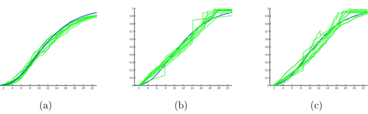
Figure 3. Estimation in Example 3, in model M7, andn= 1000. (a)-(b)-(c) beams of 20
estimators built from i.i.d. sample (thin lines) and true function (thick line): warped kernel estimators (subplot (a)), least-squares estimator in piecewise polynomial bases with degree at most 1 (subplot (b)) or 2 (subplot (c)).
the target function can be seen as a regression function: s(x) = P(Z ≤ x) =E[1Z≤x|X =x]. To
make the comparison foreseeable, the estimation set A is calibrated as it is done in Brunel and
Comte (2009), such that most of the data belong to this interval. Dierent models are considered for generating the data. We shorten "follows the distribution" by the symbol "∼".
• M1: X∼ U[0;1], andZ ∼ U[0;1],A= (0; 1)(for instance, the target function isFZ :x7→x),
• M2: X ∼ U[0;1], and Z ∼ χ2(1) (Chi-squared distribution with 1 degree of freedom), A = (0; 1),
• M3: X∼ E(1)(exponential distribution with mean 1), and Z ∼χ2(1),A= (0; 1.2),
• M4: X∼β(4,6)(Beta distribution of parameter (4,6)), Z ∼β(4,8),A= (0; 0.5),
• M5: X∼β(4,6),Z ∼ E(10) (exponential distribution with mean 0.1),A= (0; 0.5),
• M6: X∼γ(4,0.08),Z ∼ E(10),A= (0,0.5),
• M7: X∼ E(0.1),Z ∼γ(4,3),A= (1; 23).
All these models allow to investigate thoroughly the sensibility of the method to the distribution of the examination timeX, and to the range of the estimation interval. The rst two models and
the fourth were also used by Brunel and Comte (2009). Since the design is uniform in two of these examples, and also supported by the set(0; 1)in the other, we choose to explore what happens when it is not the case: in models M5, M6 and M7, the estimation interval is either smaller (M5-M6) or much larger (M7) than(0; 1). Model M3 is choosen to have a design which is not uniform.
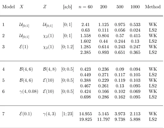
Figure 3 shows the smoothness of warped-kernel estimates compared to the reconstruction ob-tained with least-squares method. The dierence between the estimators is also investigated by computing the MISE for the dierent models. Table 3 reveals that the warped-kernel estimates can advantageously be used as soon as the design Xi has not a uniform distribution: it always
outperforms the least-squares estimators in these cases, whatever the estimation support is, and whatever the chosen distributions are. When the design is uniform, the warped-kernel strategy also leads to acceptable results but is a little less interesting (however still simpler to implement than LS methods): sinceFX(x) = x, one can clearly understand that it is not useful to warp the data.
However, recall thatFX is unknown in practice, thus we cannot assure beforehand that the warping
of the data is useless.
The practical advantages of our method are thus denitely to permit to deal with various design distributions (even very irregular ones), and thus to be stable to several data sets in dierent estimation settings (c.d.f. of current status data or regression estimation).
Model X Z [a;b] n=60 200 500 1000 Method 1 U[0;1] U[0;1] [0; 1] 2.41 1.125 0.975 0.533 WK 0.63 0.111 0.056 0.024 LS2 2 U[0;1] χ2(1) [0; 1] 1.558 0.804 0.57 0.415 WK 1.602 0.44 0.244 0.13 LS2 3 E(1) χ2(1) [0; 1.2] 1.285 0.614 0.243 0.247 WK 2.385 0.893 0.651 0.365 LS2 4 B(4,6) B(4,8) [0; 0.5] 0.423 0.236 0.09 0.094 WK 0.449 0.271 0.117 0.105 LS2 5 B(4,6) E(10) [0; 0.5] 0.388 0.229 0.119 0.103 WK 0.467 0.261 0.13 0.095 LS2 6 γ(4,0.08) E(10) [0; 0.5] 0.424 0.166 0.102 0.069 WK 0.698 0.286 0.162 0.095 LS2 7 E(0.1) γ(4,3) [1; 23] 14.955 5.145 3.973 2.113 WK 19.825 11.797 9.738 5.898 LS2
Table 3. Values of MISE×100averaged over100samples, for the estimators of the c.d.f.
from current status data (Example 3) built with the warped kernel method (WK) or the least-squares methods, with piecewise polynomials of degree at most 1 or 2 (LS1 or LS2).
5.1. Proof of Inequality (8). We have:
E[θ(Y)Kh(u−Φ(X))] = E[E[θ(Y)|X]Kh(u−Φ(X))],
=
∫
A
Kh(u−Φ(x))E[θ(Y)|X =x]fX(x)dx.
We setu′ = Φ(x), thus du′ =ϕ(x)dx. Therefore,
E[θ(Y)Kh(u−Φ(X))] = ∫ Φ(A) Kh(u−u′)E [ θ(Y)|X= Φ−1(u)]fX ( Φ−1(u)) du ϕ◦Φ−1(u), = ∫ Φ(A) Kh(u−u′)s◦Φ−1(u)du. 2
5.2. Sketch of the proof of Proposition 5.2. We need to specify the notation. The goal is to study the risk ofsˆh,h∈ Hn dened when Φis unknown. We denote it by ˆs
ˆ Φn,Φnˆ h . We have ˆ sΦnhˆ ,Φnˆ = ˆghΦnˆ ◦Φˆn, withˆg ˆ Φn h (u) = 1 n n ∑ i=1 θ(Yi)Kh ( u−Φˆn(Xi) ) .
Moreover, s˜h is denoted bysˆΦh,Φ = ˆghΦ◦Φ with gˆΦh(u) = (1/n)
∑n
i=1θ(Yi)Kh(u−Φ(Xi)) = ˜gh(u)
permits to come down to the study of˜s, is the key of the proof: ˆshΦnˆ ,Φnˆ −s 2 ϕ≤5 ∑3 l=0Tlh,with T0h =sˆhΦ,Φ−sh 2 ϕ+ sΦh −s2ϕ, T1h =sˆhΦnˆ ,Φ−sˆΦh,Φ−E [ ˆ sΦnhˆ ,Φ−sˆhΦ,Φ|(X−i)] 2 ϕ, T2h =sˆΦnhˆ ,Φnˆ −sˆΦnhˆ ,Φ−E [ ˆ sΦnhˆ ,Φnˆ −ˆshΦnˆ ,Φ|(X−i)] 2 ϕ, T3h =E [ ˆ sΦnhˆ ,Φnˆ −sˆhΦ,Φ|(X−i)] 2 ϕ,
whereE[Z|(X−i)]is the conditional expectation of a variableZ given the sample(X−i)i=1,...,n. The
term T0h has been bounded in Inequality (11). For the three others, the challenge is to prove that
they are bounded by a quantity with order of magnitude1/(nh).
Notice also that the same splitting is required to prove Theorem 3. All the details are given in Chagny (2013b).
5.3. Proof of Theorem 2. The proof is representative of the one of Theorem 3, which is thus deferred to the supplementary Chagny (2013b). Leth ∈ Hn be xed. We start with the following
decomposition for the loss of the estimator˜s= ˜s˜h: s˜˜h−s 2 ϕ = ˜gh˜−g 2 L2(Φ(A)), ≤ 3˜g˜h−g˜h,˜h 2 L2(Φ(A))+ 3 g˜h,˜h−g˜h 2 L2(Φ(A))+ 3∥g˜h−g∥ 2 L2(Φ(A)). The denitions ofA(h) and A(˜h) enable us to write, using the denition of˜h,
3˜gh˜−˜gh,˜h 2 L2(Φ(A))+ 3 g˜h,˜h−g˜h 2 L2(Φ(A)) ≤ 3 ( A(h) +V ( ˜ h )) + 3 ( A ( ˜ h ) +V(h) ) , ≤ 6 (A(h) +V(h)),
Besides, applying also (11), we obtain (22) E[˜s˜h−s2ϕ ] ≤6E[A(h)] + 6V(h) + E[θ 2(Y 1)]∥K∥2L2(R) nh + 3∥gh−g∥ 2 L2(Φ(A)). Therefore, the remainding part of the proof follows from the lemma hereafter.
Lemma 4. Leth∈ Hn be xed. Under the assumptions of Theorem 2, there exist constantsC1, C2 such that,
(23) E[A(h)]≤C1∥gh−g∥2L2(Φ(A))+
C2
n ,
where the constantC1 only depends on ∥K∥L1(R).
Applying Inequality (23) in (22) implies (16) by taking the inmum overh∈ Hn. This ends the
proof of Theorem 2.
5.4. Proof of Lemma 4. To study A(h), we introduce the auxiliary quantities gh,h′ := Kh′ ⋆
(gh1Φ(A)) =Kh′⋆((Kh⋆ g1Φ(A))1Φ(A)), for any h′ ∈ Hn, and we rst split
∥s˜h,h′−˜sh′∥2ϕ = ∥g˜h,h′−g˜h′∥2L2(Φ(A))≤3 ( Ta+Tb+∥g˜h′ −gh′∥2L2(Φ(A)) ) , (24) where Ta=∥g˜h,h′ −gh,h′∥2L2(Φ(A)), Tb =∥gh,h′ −gh′∥2L2(Φ(A)).
The rst term can be bounded as follows.
Ta ≤ Kh⋆ ( ˜ gh′1Φ(A)−gh′1Φ(A)) 2 L2(R), ≤ ∥K∥2L1(R)g˜h′1Φ(A)−gh′1Φ(A) 2 L2(R)=∥K∥ 2 L1(R)∥˜gh′−gh′∥2L2(Φ(A)),
as∥u⋆v∥L2(R)≤ ∥u∥L1(R)∥v∥L2(R)(Young convolution inequality). In the same way,Tb ≤ ∥Kh′∥2L1(R)∥gh−
g∥2L2(Φ(A)). Therefore, Decomposition (24) becomes:
∥s˜h,h′−˜sh′∥2ϕ ≤ 3∥K∥2L1(R)∥g−gh∥2L2(Φ(A))+ 3(1 +∥K∥2L1(R))∥˜gh′−gh′∥2L2(Φ(A)). Now, we get back to the denition ofA(h) given by (14):
A(h) ≤3 ∥K∥2L1(R)∥g−gh∥2L2(Φ(A)) (25) +3(1 +∥K∥2L1(R)) max h′∈Hn ( ∥˜gh′−gh′∥2L2(Φ(A))− V(h′) 3(1 +∥K∥2 L1(R)) ) + .
We can note that ∥˜gh′ −gh′∥L2(Φ(A)) = supt∈S¯(0,1)⟨˜gh′ −gh′, t⟩Φ(A), with S¯(0,1)a dense countable
subset of S˜(0,1) = {t ∈ L1(Φ(A))∩L2(Φ(A)), ∥t∥
L2(Φ(A)) = 1} (thanks to the separability of
L2(R), such a set exists. Now,
⟨˜gh′−gh′, t⟩Φ(A) = 1 n n ∑ i=1 ∫ Φ(A) {θ(Yi)Kh′(u−Φ(Xi))−E[θ(Yi)Kh′(u−Φ(Xi))]}t(u)du = νn,h′(t),
where νn,h′ is an empirical process. Thus, thanks to (25), it remains to bound the deviations of
supt∈S¯(0,1)νn,h2 ′(t). First, we have
E [ max h′∈Hn ( sup t∈S¯(0,1) νn,h2 ′(t)− V(h ′) 3(1 +∥K∥2L1(R)) ) + ] ≤ ∑ h′∈Hn E [( sup t∈S¯(0,1) νn,h2 ′(t)− V(h ′) 3(1 +∥K∥2L1(R)) ) + ] .
Then, the conclusion results from the following lemma:
Lemma 5. Under the assumptions of Theorem 2, there exists a constant C such that,
∑ h∈Hn E [( sup t∈S¯(0,1) νn,h2 (t)−V˜(h) ) + ] ≤ C n, with V˜(h) =δ′∥K∥ L2(R)E[θ(Y1)2]/(nh) for a numerical δ′>0.
We choose the constantκinvolved in the denition ofV such thatV˜(h)≤V(h)(1 +∥K∥2L1(R))/3. Thus, the proof is complete.
5.5. Proof of Lemma 5. We write the empirical process νn,h(t) = 1 n n ∑ i=1 ψt,h(Xi, Yi)−E[ψt,h(Xi, Yi)], (26) withψt,h(Xi, Yi) =θ(Yi) ∫ Φ(A) Kh(u−Φ(Xi))t(u)du.
The guiding idea is to apply the Talagrand Inequality, in its version given in Klein and Rio (2005). We will use the notations used in Lemma 5 of Lacour (2008) (p.812). Ifθis bounded, this inequality
can be applied. Otherwise, we have to introduce a truncation.
5.5.1. Example 1. Recall thatΦ =FX andΦ(A) = [0; 1]. We split the processνn,hinto three parts,
writingνn,h=ν (1) n,h+ν (2,1) n,h +ν (2,2) n,h , with, for l= 1,(2,1),(2,2), νn,h(l) = 1 n n ∑ i=1 φ(t,hl)(Zi)−E [ φ(t,hl)(Zi) ] , Zi=Xi or (Xi, εi), and φ(1)t,h : x 7→ s(x)∫01Kh(u−FX(x))t(u)du, φ(2t,h,1) : (x, ε) 7→ ε1|ε|≤κn ∫1 0 Kh(u−FX(x))t(u)du, φt,h(2,2) : (x, ε) 7→ ε1|ε|>κn∫01Kh(u−FX(x))t(u)du,
where we dene, for a constantc which will be specied below,
(27) κn=c
√
n
ln(n).
We apply Talagrand's Inequality to the rst two bounded empirical processes, and bound roughly the last one. Thus, we split:
∑ h∈Hn E [( sup t∈S¯(0,1) νn,h2 (t)−V˜(h) ) + ] ≤ 3 ∑ h∈Hn { E [( sup t∈S¯(0,1) ( νn,h(1)(t) )2 − V˜1(h) 3 ) + ] (28) +E [( sup t∈S¯(0,1) ( νn,h(2,1)(t) )2 −V˜2(h) 3 ) + ] +E [ sup t∈S¯(0,1) ( νn,h(2,2)(t) )2]} ,
with the decompositionV˜(h) = ˜V1(h) + ˜V2(h), and, denoting byδ′′=δ′/2, ˜ V1(h) = 3δ′′ ∥K∥2L2(R)E [ s2(X1) ] nh , and V˜2(h) = 3δ ′′∥K∥2L2(R)E [ ε21] nh .
Actually, recall that we have E[θ2(Y1)] =E[Y12] =E[s2(X1)] +E[ε21]here.
We now show that each of the three terms of the right hand-side of (28) is upper-bounded by a quantity of order1/n. This will end the proof.
• First term of (28).
Let us begin withνn,h(1). To do so, we computeH(1),M(1)andv(1), involved in Lemma 5 of Lacour
• ForM(1), lett∈S¯(0,1)and x∈A be xed: φ(1)t,h(x) ≤ |s(x)| ∫ 1 0 |Kh(u−FX(x))t(u)|du≤ |s(x)|∥Kh∥L2(R)∥t∥L2(Φ(A)), = |s(x)|∥K√∥L2(R) h ≤ ∥s∥L∞(A) ∥K∥L2(R) √ h :=M (1).
• ForH(1), notice that
νn,h(1)(t) =⟨dˆh−gh, t⟩Φ(A), with dˆh = 1 n n ∑ i=1 s(Xi)Kh(.−FX(Xi)).
Thus, thanks to the Young convolution inequality, we obtain,
E [ sup t∈S¯(0,1) ( νn,h(1)(t) )2] = E [ dˆh−gh2 L2([0;1]) ] , = ∫ 1 0
Var(dˆh(u))du, since gh(u) =E[dˆh(u)],
≤ ∫ 1 0 1 nE [ s2(X1)Kh2(u−FX(X1)) ] du.
Then, we use the same computation as the one done to bound the variance term in the proof of (11), and set(H(1))2 =∥K∥2L2(R)E[s2(X1)]/(nh).
• Forv(1), we also xt∈S¯(0,1). Hereafter, we setKˇh(u) =Kh(−u). First,
Var(φ(1)t,h(X1) ) ≤ E[(φ(1)t,h(X1) )2] ≤ ∥s∥2L∞(A)E [(∫ 1 0 Kh(u−FX(X1))t(u)du )2] ,
and the expectation can be written
E[(∫ 1 0 Kh(u−FX(X1))t(u)du )2] = E[(Kˇh∗ ( t1[0;1] ))2 (FX(X1)) ] , = ∫ 1 0 (ˇ Kh∗ ( t1[0;1] ))2 (u)du≤Kˇh∗ ( t1[0;1]) 2 L2(R), ≤ Kˇh2 L1(R)∥t1[0;1]∥L22(R)=Kˇh 2 L1(R)∥t∥ 2 L2([0;1]), thanks to the Young convolution inequality. Therefore,
Var(φ(1)t,h(X1) )
≤ ∥s∥L∞(A)∥K∥2L1(R):=v(1). Then, Talagrand's Inequality gives, forδ >0,
E [( sup t∈S¯(0,1) ( νn,h(1)(t) )2 −2(1 + 2δ) ( H(1) )2) + ] ≤k1 { 1 nexp ( −k2 1 h ) + 1 n2hexp ( −k3 √ n)},
wherek1, k2, k3 are three constants which depend onE[s2(X1)],∥s∥L∞(A),∥K∥L1(R) and∥K∥L2(R). Assumptions (H2)-(H3) lead to ∑ h∈Hn E [( sup t∈S¯(0,1) ( νn,h(1)(t) )2 −2(1 + 2δ)∥K∥2L2(R)E[s2(X1)] 1 nh ) + ] ≤ C n,
withC a constant (which also depends on the previous quantities).
For the second empirical processνn,h(2,1), the sketch of the proof is the same: similarly, we compute
the quantities involved in the Talagrand Inequality,
M(2) =κn∥K∥L2(R) 1 √ h, H (2) =∥K∥ L2(R) ( E[ε21])1/2√1 nh, v (2)=∥K∥2 L1(R)E[ε21], and we obtain, by Lemma 5 of Lacour (2008) (p.812), forδ >0,
E [( sup t∈S¯(0,1) ( νn,h(2,1)(t) )2 −2(1 + 2δ) ( H(2) )2) + ] ≤k1 { 1 nexp ( −k2 1 h ) + κ 2 n n2hexp ( −k3 √ n κn )} ,
wherek1, k2, k3 are three constants which depend onE[ε21],∥K∥L1(R) and∥K∥L2(R). The rst term of the right hand-side is like above. With the denition (27) of κn, the sum over h ∈ Hn of the
second term of the upper bound can be written ∑ h∈Hn κ2 n n2hexp ( −k3 √ n κn ) = c 2 n1+k3/cln2(n) ∑ h∈Hn 1 h.
Consequently, using Assumptions (H2)-(H3) and choosing c in the denition of κn such that c ≤
k3/α0, we also obtain for a constantC, ∑ h∈Hn E [( sup t∈S¯(0,1) ( νn,h(2,1)(t) )2 −2(1 + 2δ)∥K∥2L2(R)E[ε21] 1 nh ) + ] ≤ C n. • Third term of (28).
The last empirical process isνn,h(2,2)(t) =∫01t(u)ψ(u)du, with
ψ(u) = 1 n n ∑ i=1 εi1{|εi|>κn}Kh(u−FX(Xi))−E [ εi1{|εi|>κn}Kh(u−FX(Xi)) ] .
It is not bounded. Nevertheless, we use the Cauchy-Schwarz Inequality, and the equality∥t∥L2(Φ(A))= 1, for t∈S¯(0,1) E [ sup t∈S˜(0,1) ( νn,h(2,2)(t) )2] ≤ E [∫ 1 0 ψ2(u)du ] , ≤ 1 nE [ ε211{|ε1|>κn} ] E [∫ 1 0 Kh2(u−FX(X1))du ] , ≤ ∥K∥ 2 L2(R) nh E [ ε211{|ε1|>κn} ] ≤ ∥K∥ 2 L2(R)κ− p n nh E [ ε2+1 p ] .
Thus, there exists a constantk1 which depends on∥K∥L2(R) and E[ε2+1 p], ∑ h∈Hn E [ sup t∈S¯(0,1) ( νn,h(2,2)(t) )2] ≤k1 κ−np n ∑ h∈Hn 1 h =c1κ −plnp(n) n1+p/2 ∑ h∈Hn 1 h.
The conclusion comes from Assumptions (H2)-(H3), and the choice ofp≥2α0.