The value of tax shields with a fixed book-value leverage ratio
30
0
0
Full text
(2) The CIIF, International Center for Financial Research, is an interdisciplinary center with an international outlook and a focus on teaching and research in finance. It was created at the beginning of 1992 to channel the financial research interests of a multidisciplinary group of professors at IESE Business School and has established itself as a nucleus of study within the School’s activities. Ten years on, our chief objectives remain the same: •. Find answers to the questions that confront the owners and managers of finance companies and the financial directors of all kinds of companies in the performance of their duties. •. Develop new tools for financial management. •. Study in depth the changes that occur in the market and their effects on the financial dimension of business activity. All of these activities are programmed and carried out with the support of our sponsoring companies. Apart from providing vital financial assistance, our sponsors also help to define the Center’s research projects, ensuring their practical relevance. The companies in question, to which we reiterate our thanks, are: Aena, A.T. Kearney, Caja Madrid, Fundación Ramón Areces, Grupo Endesa, Telefónica and Unión Fenosa. http://www.iese.edu/ciif/.
(3) THE VALUE OF TAX SHIELDS WITH A FIXED BOOK-VALUE LEVERAGE RATIO. Abstract The value of tax shields depends only on the nature of the stochastic process of the net increases of debt. The value of tax shields in a world with no leverage cost is the tax rate times the current debt plus the present value of the net increases of debt. We develop valuation formulae for a company that maintains a fixed book-value leverage ratio and show that it is more realistic than to assume, as Miles-Ezzell (1980) do, a fixed market-value leverage ratio. We also show that Miles-Ezzell assume that the increase of debt is proportional to the increase of the free cash flows.. JEL classification: G12; G31; G32. Keywords: Value of tax shields, present value of the net increases of debt, required return to equity.
(4) THE VALUE OF TAX SHIELDS WITH A FIXED BOOK-VALUE LEVERAGE RATIO. There is no consensus in the existing literature regarding the correct way to compute the value of tax shields. Most authors think of calculating the value of the tax shield in terms of the appropriate present value of the tax savings due to interest payments on debt, but Modigliani-Miller (1963) propose to discount the tax savings at the risk-free rate1, whereas Harris and Pringle (1985) propose discounting these tax savings at the cost of capital for the unlevered firm. Miles and Ezzel (1985) propose discounting these tax savings the first year at the cost of debt and the following years at the cost of capital for the unlevered firm. Reflecting this lack of consensus, Copeland et al. (2000, p. 482) claim that “the finance literature does not provide a clear answer about which discount rate for the tax benefit of interest is theoretically correct.” We show that the value of tax shields depends only upon the nature of the stochastic process of the net increase of debt. More specifically, we prove that the value of tax shields in a world with no leverage cost is the tax rate times the current debt, plus the tax rate times the value of the future net increases of debt. By applying this formula to specific situations, we show that the Modigliani-Miller (1963) formula should be used when the company has a preset amount of debt; Fernández (2004), when the company expects the increases of debt to be as risky as the free cash flows (for example, if the company wants to maintain a fixed book-value leverage ratio); and Miles-Ezzell (1980), only if debt will be always a multiple of the equity market value (Dt = L·St). We will argue that although Dt = L·St provides a computationally elegant solution, it is not a realistic one. What is more, we have not seen any company that follows this financing policy. It makes much more sense to characterize the debt policy of a company with expected constant leverage ratio as a fixed book-value leverage ratio rather than as a fixed market-value leverage ratio because 1. the debt does not depend on the movements of the stock market, 2. it is easier to follow for unlisted companies, and 3. managers should prefer it because the value of tax shields is higher.. I thank my colleagues José Manuel Campa and Charles Porter for their wonderful help revising earlier manuscripts of this paper, and an anonymous referee for very helpful comments. I also thank Rafael Termes and my colleagues at IESE for their sharp questions that encouraged me to explore valuation problems. 1. Myers (1974) proposes to discount it at the cost of debt (Kd)..
(5) 2 Although Cooper and Nyborg (2006) disagree, this paper shows that Fernández’s (2004) formula (28) (VTS = PV[Ku; D·T·Ku]) is valid, but only under the assumption that the increases of debt are as risky as the free cash flows. The paper is organized as follows. In section 1 we derive the general formula for the value of tax shields. In section 2 we apply this formula to specific situations. Section 3 discusses the opinions of other authors. In section 4 we calculate the value of taxes for the levered and the unlevered firm. Section 5 is a numerical example. Section 6 presents the valuation formulae for finite horizons. Section 7 discusses the influence of growth on the risk of the cash flows. Section 8 concludes. To avoid arguments about the appropriate discount rates, we will use pricing kernels. The price of an asset that pays a random amount xt at time t is the sum of the expectation of the product of xt and Mt, the pricing kernel for time t cash flows: ∞. Px = ∑ E[M t ·x t ]. (1). 1. 1. General expression of the value of tax shields The value of the debt today (D0) is the value today of the future stream of interest minus the value today of the future stream of the increases of debt (∆Dt): ∞. ∞. 1. 1. D 0 = ∑ E[M t ·Interest t ] − ∑ E[M t ·∆D t ]. (2). As the value of tax shields is the value of the interest times the tax rate, ∞. ∞. 1. 1. VTS0 = T ∑ E[M t ·Interest t ] = T·D 0 + T ∑ E[M t ·∆D t ]. (3). Equation (3) is valid for perpetuities and for companies with any pattern of growth. More importantly, this equation shows that the value of tax shields depends only upon the nature of the stochastic process of the net increase of debt. The problem of equation (3) is how to calculate the value today of the increases of debt. The value today of the levered company (VL0) is equal to the value of debt (D0) plus the value of the equity (S0). It is also equal to the value of the unlevered company (Vu0)2 plus the value of tax shields due to interest payments (VTS0): VL0 = S0 + D0 = Vu0 + VTS0. (4). In the literature, the value of tax shields defines the increase in the company’s value as a result of the tax saving obtained by the payment of interest.. 2. ∞. ∞. 1. 1. According to our notation, Vu 0 = ∑ E[M t ·FCFt ] and S 0 = ∑ E[M t ·ECFt ] , where FCFt is the free cash flow. of period t, and ECFt is the equity cash flow of period t..
(6) 3. 2. Value of the increases of debt and value of tax shields in specific situations We apply the result in (3) to specific situations and show how this formula is consistent with previous formulae under restrictive scenarios. We will assume that FCFt+1 = FCFt (1 + g)(1 + εt+1). (5). εt+1 is a random variable with expected value equal to zero (Et[εt+1] = 0), but with a value today smaller than zero:. [. ]. E t M t ,t +1 ·ε t +1 = −. d 1+ RF. (6). The risk free rate corresponds to the following equation: ∞ 1 = ∑ E[M t ·1] 1+ RF 1. (7). First, we deduct the value of the unlevered equity. If Mt,t+1 is the one-period pricing kernel at time t for cash flows at time t+1, Vu t = E t [M t ,t +1 ·FCFt +1 ] + E t [M t ,t +1 ·Vu t +1 ]. (8). A solution must be Vut = a·FCFt; then:. [. ]. [. ]. [. Vu t = E t M t ,t +1 ·FCFt +1 + E t M t,t +1 ·aFCFt +1 = (1 + a ) E t M t ,t +1 ·FCFt +1. ]. (9). According to (5): E t [M t ,t +1 ·FCFt +1 ] = E t [M t ,t +1 ·FCFt (1 + g )] + E t [M t ,t +1 ·FCFt (1 + g )ε t +1 ]. (10). Using equation (6) and defining Ku = (RF + d) / (1 - d):. [. ]. E t M t ,t +1 ·FCFt +1 =. FCFt (1 + g) FCFt (1 + g)d FCFt (1 + g)(1 − d ) FCFt (1 + g) − = = 1+ RF 1+ RF 1+ RF 1 + Ku Vu t = aFCFt = (1 + a ) a=. FCFt (1 + g) 1 + Ku. (1 + g) Ku − g. (11) (12) (13). Then: ∞. Vu t = ∑ E[M t ·FCFt ] = 1. (1 + g) FCFt Ku − g. (14).
(7) 4. 2.1. Debt is proportional to the equity book value If Dt = K·Ebvt, where Ebv is the book value of equity, then ∆Dt = K·∆Ebvt. The increase of the book value of equity is equal to the profit after tax (PAT) minus the equity cash flow (ECF). The relationship between the profit after tax of the levered company (PATL) and the equity cash flow (ECF) is: ECFt = PATLt – ∆At + ∆Dt. (15). Notation being, ∆At = Increase of net assets in period t (Increase of Working Capital Requirements plus Increase of Net Fixed Assets); ∆Dt = Dt – Dt-1 = Increase of Debt in period t. Similarly, the relationship between the profit after tax of the unlevered company (PATu) and the free cash flow (FCF) is: FCFt = PATut – ∆At. (16). According to equation (15) ∆Ebvt = PATLt – ECFt = ∆At – ∆Dt = ∆Dt / K. (17). In this situation, the increase of debt is proportional to the increases of net assets and the risk of the increases of debt is equal to the risk of the increases of assets: ∆Dt = ∆At / (1+1/K). (18). The value today of the increases of debt is:. [. ]. [. ⎛ K ⎞ E 0 M 0,t ·∆D t = ⎜ ⎟ E 0 M 0,t ·∆A t ⎝1+ K ⎠. ]. (19). We will assume that the increase of net assets follows the stochastic process defined by ∆At+1 = ∆At (1+g)(1+φt+1). φt+1 is a random variable with expected value equal to zero (Et[φt+1] = 0), but with a value today smaller than zero:. [. ]. E t M t ,t +1 ·φ t +1 = −. f 1+ RF. (20). Then, in the case of a growing perpetuity: t t ⎛ K ⎞ (1 + g ) (1 − f ) E 0 M 0,t ·∆D t = ∆A 0 ⎜ ⎟ ⎝ 1 + K ⎠ (1 + R F ) t. [. ]. (21). If we call (1+α) = (1+RF) / (1-f), then. [. ]. E 0 M 0,t ·∆D t = ∆D 0. (1 + g) t. (22). (1 + α) t ∞. α is the appropriate discount rate for the expected increases of debt. ∑ E[M t ∆D t ] is 1. the sum of a geometric progression with growth rate = (1+g)/(1+α)..
(8) 5. Then: ∞. ∑ E[M t ∆D t ] = 1. ∆D 0 (1 + g) ∆D 0 (1 + g) gD 0 = = 1 + g (1 + α) α−g α−g 1− 1+ α. (23). Substituting (23) in (3), we get: VTS 0 =. D0α T ( α − g). (24). 2.2. Debt is proportional to the Equity book value and the increase of assets is proportional to the free cash flow In this situation, ∆At+1 = Z·FCFt, and equation (19) is:. [. ]. [. ]. [. ⎛ K ⎞ ⎛ K ⎞ E 0 M 0,t ·∆D t = ⎜ ⎟ Z·E 0 M 0,t ·FCFt ⎟ E 0 M 0,t ·∆A t = ⎜ ⎝1+ K ⎠ ⎝1+ K ⎠. ]. (25). This is equivalent to assuming that φt+1 = εt+1. Then f = d, and α = Ku. According to equation (14): ∞. g· D 0 ⎛ K ⎞ (1 + g ) FCF0 ⎛ K ⎞ ∞ = ⎟Z ⎟ Z·∑ E[M t ·FCF t ] = ⎜ Ku − g Ku − g ⎝1 + K ⎠ ⎝1 + K ⎠ 1. ∑ E [M t ∆ D t ] = ⎜ 1. (26). Substituting (26) in (3), we get: VTS 0 =. D 0 Ku T ( Ku − g). (27). If we assume that the increases of debt are as risky as the free cash flows (α = Ku), the correct discount rate for the expected increases of debt is Ku, the required return to the unlevered company. (27) is equal to equation (28) in Fernández (2004).3 2.3. The company has a preset amount of debt In this situation, ∆Dt is known with certainty today.. [. ]. E 0 M 0,t ·∆D t = ∆D 0. (1 + g ) t (1 + R F ). (28) t. ∞. ∑ E[M t ∆D t ]. is the sum of a geometric progression with growth rate (1+g)/(1+RF). 1. 3. Fernández (2004) neglected to include in Equations (5) to (14) terms with expected value equal to zero. And he wrongly considered as being zero the present value of a variable with expected value equal to zero. Due to these errors, Equations (5) to (17), Tables 3 and 4, and Figure 1 of Fernández (2004) are correct only if PV0[∆At] = PV0[∆Dt] = 0..
(9) 6 Then: ∞. ∑ E[M t ∆D t ] = 1. ∆D 0 ∆D 0 (1 + g ) gD 0 (1 + g) = = 1 + g (1 + R F ) RF − g RF − g 1− 1+ RF. (29). Substituting (29) in (3), we get: VTS0 =. D0 R F T ( R F − g). (30). In this case, Modigliani-Miller (1963) applies: the appropriate discount rate for the ∆Dt (known with certainty today) is RF, the risk-free rate. Note that, in the case of a growing perpetuity, Modigliani-Miller may be viewed as just one extreme case of section 2.2, in which α = RF. 2.4. Debt is proportional to the Equity market value This is the assumption made by Miles and Ezzell (1980) and Arzac and Glosten (2005). If Dt = L·St, VLt = S t + D t =. Dt 1+ L Dt + Dt = L L. (31). We prove in Appendix 1 that the value today of the increase of debt in period 1, if the debt grows at a constant rate g, is:. [. ]. E 0 M 0,1 ·∆D1 =. D 0 (1 + g) D0 − 1 + Ku 1+ RF. (32). We also prove that for t > 1:. [. ]. E 0 M 0,t ·∆D t = D 0. ⎞ (1 + g) t −1 ⎛ (1 + g) 1 ⎜ ⎟ − t −1 ⎜ (1 + Ku ) (1 + R ) ⎟ (1 + Ku ) ⎝ F ⎠. (33). ∞. ∑ E[M t ∆D t ]. is the sum of a geometric progression with growth rate (1+g)/(1+Ku). 1. Then: ∞. ∑ E[M t ∆D t ] = 1. D0 ⎛ Ku − R F ⎜⎜ g − Ku − g ⎝ 1+ RF. ∞. ⎞ ⎟⎟ ⎠. (34). Ku − R. F Note that, under Miles-Ezzell ∑ E[M t ∆D t ] < 0 if g < 1 + R F 1. Substituting (34) in (3), we get: VTS 0 =. D 0 R F T (1 + Ku) (Ku − g) (1 + R F ). (35). It makes more sense to characterize the debt policy of a growing company with expected constant leverage ratio as a fixed book-value leverage ratio instead of as a fixed market-value leverage ratio because:.
(10) 7 1. the debt does not depend on the movements of the stock market, 2. it is easier to follow for non-quoted companies, and 3. managers should prefer it because the value of tax shields is higher: (35) is smaller than (27) and than (24). To assume Dt = L·Et is not a good description of the debt policy of any company because if a company has only two possible states of nature in the following period, it is clear that under the worst state (low share price) the leveraged company will have to raise new equity and repay debt, and this is not the moment companies prefer to raise equity. Under the good state, the company will have to take a lot of debt and pay big dividends. The Miles-Ezzell setup works as if the company pays all the debt (Dt-1) at the end of every period t and simultaneously raises all new debt Dt. The risk of raising the new debt is similar to the risk of the free cash flow and, hence, the appropriate discount rate for the expected value of the new debt is Ku. Dt = L·St may be a computationally elegant solution (as shown in Arzac-Glosten, 2005), but unfortunately not a realistic one. Furthermore, we have not seen any company that follows this financing policy. In Appendix 1 we also prove that if Dt = L·St, then the increase of debt is proportional to the increase of the free cash flows.. 3. Value of net increases of debt implied by other authors Table I summarizes the implications of several approaches for the value of tax shields and for the value of the future increases of debt. As we have already argued, Modigliani-Miller (1963) should be used when the company has a preset amount of debt; Fernández (2004), when we expect the increases of debt to be as risky as the free cash flow (for example, if the company wants to maintain a fixed book-value leverage ratio); and Miles-Ezzell (1980), only if debt will be a multiple of the equity market value Dt = L·Et. If the company maintains a fixed book-value leverage ratio and the risk of the increases of assets is different than the risk of the free cash flow, then the formulas of section 2.3 (and Appendix 2) should be applied. Fieten et al. (2005) argue that the Modigliani-Miller formula may be applied to all situations. We have shown that it is valid only when the company has a preset amount of debt. Cooper and Nyborg (2006) affirm that equation (27) violates value-additivity. It does not because equation (4) holds. They use only the cost of debt (RF) or the cost of the unlevered equity (Ku) to discount the expected value of tax shields. We have seen that there are also other debt policies, for example, when the firm wants to maintain a fixed bookvalue leverage ratio..
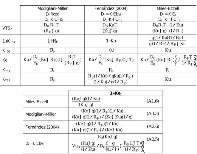
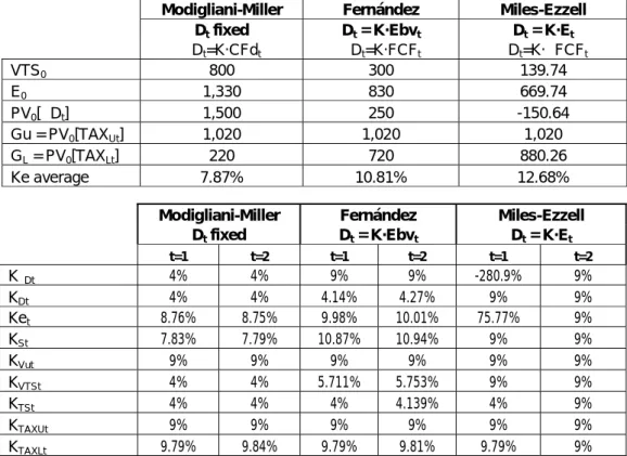
(11) 8. 4. Value today of the expected taxes If leverage costs do not exist, then Eq. (4) could be stated as follows: Vu0 + Gu0 = S0 + D0 + GL0. (36). where Gu0 is the value today of the taxes paid by the unlevered company and GL0 is the value today of the taxes paid by the levered company. Eq. (36) means that the total value of the unlevered company (left-hand side of the equation) is equal to the total value of the levered company (right-hand side of the equation). Total value is the enterprise value (often called the value of the firm) plus the value today of taxes. Eq. (36) assumes that expected free cash flows are independent of leverage4. From (4) and (36), it is clear that the value of tax shields (VTS) is VTS0 = Gu0 – GL0 (37) The taxes paid every year by the unlevered company (TaxesU) are TaxesUt = [T/(1-T)] PATu = [T/(1-T)] (FCFt + ∆At). (38). For the levered company, taking into consideration Eq. (17), the taxes paid each year (TaxesL) are: TaxesLt = [T/(1-T)] (ECFt + ∆At -∆Dt). (39). The present values at t=0 of equations (38) and (39) are: ∞ ∞ ⎞ ⎛ T ⎞⎛ ⎞ ⎛ T ⎞⎛⎜ ∞ Gu 0 = ⎜ ⎟⎜ ∑ E[M t ·FCFt ] + ∑ E[M t ·∆A t ]⎟⎟ = ⎜ ⎟⎜⎜ Vu 0 + ∑ E[M t ·∆A t ]⎟⎟ ⎝ 1 − T ⎠⎝ 1 1 1 ⎠ ⎝ 1 − T ⎠⎝ ⎠. (40). ∞ ∞ ⎞ ⎛ T ⎞⎛⎜ ∞ G L0 = ⎜ ⎟⎜ ∑ E[M t ·ECFt ] + ∑ E[M t ·∆A t ] − ∑ E[M t ·∆D t ]⎟⎟ ⎝ 1 − T ⎠⎝ 1 1 1 ⎠. (41). The value of tax shields is the difference between Gu (40) and GL (41).. 5. A numerical example and a closer look at the discount rates Appendixes 1, 2 and 3 derive additional formulae for the three theories discussed in this paper applied to growing perpetuities. Table II is a summary of the main formulae. Table III contains the main valuation results for a constant growing company. It is interesting to note that, according to Miles-Ezzell, the value today of the increases of debt is negative. According to Modigliani-Miller, Ke < Ku. It is interesting to note that while two theories assume a constant rate for the increases of debt (Modigliani-Miller assumes RF and Fernández assumes Ku), Miles-Ezzell assumes one rate for t = 1 and Ku for t>1. The appropriate discount rate for the increase of debt in t = 1 is, according to Miles-Ezzell, equation (A1.9): 1 + K ∆D1 = 4. g (1 + Ku) (1 + R F ) g (1 + R F ) + R F − Ku. When leverage costs do exist, the total value of the levered company is lower than the total value of the unlevered company. A world with leverage cost is characterized by the following relation: Vu + Gu = S + D + GL + Leverage Cost > S + D + GL Leverage cost is the reduction in the company’s value due to the use of debt..
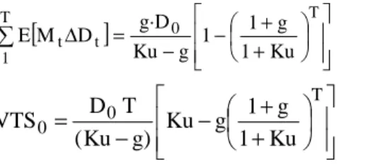
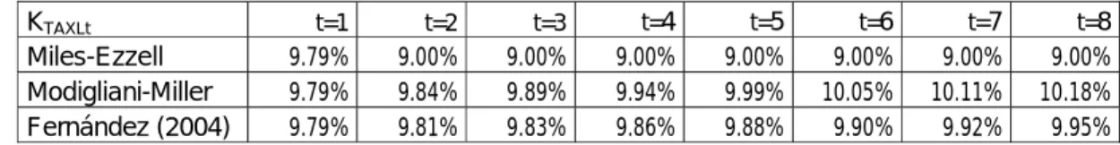
(12) 9 In our example, K∆D1 = –280.9%. Table IV contains the value of the tax shields (VTS) according to the different theories as a function of g and α. The results change dramatically when g increases. It may be seen that Modigliani-Miller is equivalent to a constant book-value leverage ratio (Dt = L·Ebvt), when α= RF = 4%. The VTS according to M-M is infinite when g > RF. Fernández (2004) is equivalent to Dt = L·Ebvt when α = Ku = 9%. Table V contains the value today of the increases of debt in different periods and the sum of all of them. According to Miles-Ezzell, the value today of the increases of debt in every period is negative. We also prove that although the equity value of a growing perpetuity can be computed by discounting the expected value of the equity cash flow with a single rate Ke, the appropriate discount rates for the expected values of the equity cash flows are not constant. Table VI presents the appropriate discount rates for the expected values of the equity cash flows of our example. According to Miles-Ezzell, Ket is 75.77% for t = 1 and 9% for the rest of the periods. According to Modigliani-Miller, Ket < Ku = 9%. We also derive the appropriate discount rates for the expected values of the taxes. If we assume that the appropriate discount rate for the increases of assets is Ku, then the appropriate discount rate for the expected value of the taxes of the unlevered company is also Ku. But the appropriate discount rate for the expected value of the taxes of the levered company (KTAXL) is different according to the three theories. Table VII presents the appropriate discount rates for the expected values of the taxes in the initial periods for our example. According to Miles-Ezzell, KTAXLt is 9.79% for t = 1 and 9% for the rest of the periods. According to the other theories, KTAXLt is higher than Ku (9%) and grows with t. According to Modigliani-Miller and according to Fernández, the taxes of the levered company are riskier than the taxes of the unlevered company. However, according to Miles-Ezzell, both taxes are equally risky for t > 1.5. 6. Valuation formulae for finite horizons We have developed formulae for perpetuities. In this section, we show the main valuation formulae for a growing company that will produce cash flows only until period t=T. Today is t=0. In the case of a company that maintains a fixed book-value leverage ratio, the value today of the increases of debt and the value of tax shields are6: T. ∑ E[M t ∆D t ] = 1. T gD 0 ⎡ ⎛ 1 + g ⎞ ⎤ ⎢1 − ⎜ ⎟ ⎥ α − g ⎢ ⎝1+ α ⎠ ⎥ ⎣ ⎦. T D0 T ⎡ ⎛ 1+ g ⎞ ⎤ ⎢α − g⎜ VTS 0 = ⎟ ⎥ ( α − g) ⎢ 1+ α ⎠ ⎥ ⎝ ⎣ ⎦. 5. (23T) (24T). If the risk of the increase of assets is smaller than the risk of the free cash flows, then Miles-Ezzell provides a surprising result: the taxes of the levered company are less risky than the taxes of the unlevered company. 6 The numbers of the formulae in this section are the same as in previous sections: we merely add a T..
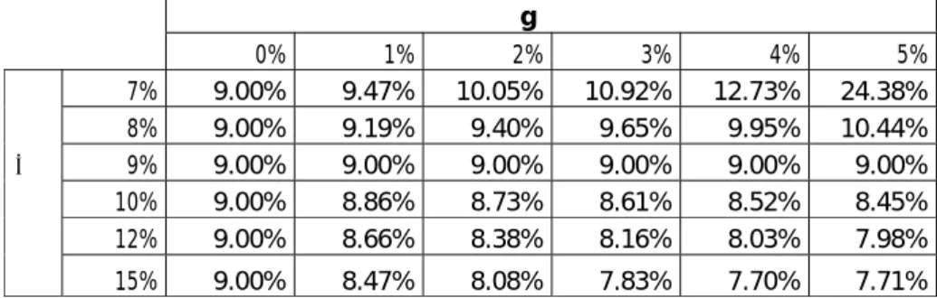
(13) 10 If the company maintains a fixed book-value leverage ratio, and the increases of assets are as risky as the free cash flows, the value today of the increases of debt and the value of tax shields are: T. ∑ E[M t ∆D t ] = 1. VTS 0 =. T g·D 0 ⎡ ⎛ 1 + g ⎞ ⎤ ⎢1 − ⎜ ⎟ ⎥ Ku − g ⎢ ⎝ 1 + Ku ⎠ ⎥ ⎣ ⎦. T D0 T ⎡ ⎛ 1+ g ⎞ ⎤ ⎢ Ku − g⎜ ⎟ ⎥ ( Ku − g) ⎢ ⎝ 1 + Ku ⎠ ⎥⎦ ⎣. (26T). (27T). If we assume that the increases of debt are riskless, the value today of the increases of debt and the value of tax shields are: T. ∑ E[M t ∆D t ] = 1. gD 0 ⎡ ⎛ 1 + g ⎢1 − ⎜ R F − g ⎢ ⎜⎝ 1 + R F ⎣. ⎞ ⎟⎟ ⎠. T⎤. ⎥ ⎥ ⎦. T ⎛ 1+ g ⎞ ⎤ D0 T ⎡ ⎢ ⎟ ⎥ VTS 0 = R F − g⎜⎜ ( R F − g) ⎢ 1 + R F ⎟⎠ ⎥ ⎝ ⎣ ⎦. (29T) (30T). Under Miles-Ezzell: T. ∑ E[M t ∆D t ] = 1. VTS 0 =. D0 ⎛ Ku − R F ⎜⎜ g − Ku − g ⎝ 1+ RF. ⎞⎡ ⎛ 1 + g ⎞ T ⎤ ⎟⎟ ⎢1 − ⎜ ⎟ ⎥ ⎠ ⎢⎣ ⎝ 1 + Ku ⎠ ⎥⎦. T⎞ ⎛ D0 T ⎜ R (1 + Ku) - [Ku − R − g(1 + R )]⎛⎜ 1 + g ⎞⎟ ⎟ F F F (Ku − g)(1 + R F ) ⎜ ⎝ 1 + Ku ⎠ ⎟⎠ ⎝. (34T) (35T). 7. Is Ku independent of growth? Up to now we have assumed that Ku is constant, independent of growth. From equation (6) we know that FCFt = PATut - ∆At. If we consider that the risk of the unlevered profit after tax (PATu) is independent of growth, and that KPATu is the required return to the expected PATu, the present value of equation (6) is: Vu 0 =. (1 + g) FCF0 (1 + g) PATu 0 gA 0 = − ( Ku − g ) ( K PATu − g) ( α − g). Ku = g +. (1 + g ) FCF0 (1 + g ) PATu 0 gA 0 − ( K PATu − g ) ( α − g ). Table VIII contains the required return to the free cash flows (Ku) as a function of α (required return to the increase of assets) and g (expected growth). It may be seen that Ku is increasing in g7 if α < KPATu, and decreasing in g if α > KPATu. 7. This result contradicts Cooper and Nyborg (2006), who maintain that “Ku is decreasing in g”..
(14) 11. 8. Conclusions The value of tax shields depends only upon the nature of the stochastic process of the net increase of debt. More specifically, the value of tax shields in a world with no leverage cost is the tax rate times the current debt, plus the tax rate times the value today of the net increases of debt. This expression is equivalent to the difference between the present values of two different cash flows, each with its own risk: the value today of taxes for the unlevered company and the value today of taxes for the levered company. The critical parameter for calculating the value of tax shields is the value today of the net increases of debt. It may vary for different companies, but it may be calculated in specific circumstances. For perpetual debt, the value of tax shields is equal to the tax rate times the value of debt. When the debt level is fixed, Modigliani-Miller (1963) applies, and the value of tax shields is the value today of the tax shields, discounted at the required return to debt. If the leverage ratio (D/E) is fixed at market value, then Miles-Ezzell (1980) applies with the caveats discussed. If the leverage ratio is fixed at book values and the increases of assets are as risky as the free cash flows (the increases of debt are as risky as the free cash flows), then Fernández (2004) applies. We have developed new formulas for the situation in which the leverage ratio is fixed at book values but the increases of assets have a different risk than the free cash flows. We argue that it is more realistic to assume that a company maintains a fixed bookvalue leverage ratio than to assume, as Miles-Ezzell (1980) do, that the company maintains a fixed market-value leverage ratio..
(15) 12 Table I Value today of the increases of debt implicit in the most popular formulae for calculating the value of tax shields. Perpetuities growing at a constant rate g ∞. Authors. VTS0. PV0[∆Dt]= ∑ E[M t ∆D t ]. Miles-Ezzell (1980) Arzac-Glosten (2005). D 0 R F T (1 + Ku ) (Ku − g) (1 + R F ). D 0 ⎛ Ku - R F ⎜g Ku − g ⎜⎝ 1+ RF. Modigliani-Miller (1963). D0 R F T (R F − g). g·D 0 RF − g. D 0 Ku T (Ku − g) D0 α T (α − g). g·D0 Ku − g g·D 0 α−g. 1. Fernández (2004) Constant book-value leverage. ⎞ ⎟⎟ ⎠. Ku = unlevered cost of equity T = corporate tax rate D0 = debt value today RF = risk-free rate α = required return to the increases of assets. Table II Main formulas in the appendixes for growing perpetuities. VTS0. Modigliani-Miller Dt fixed ∆Dt=K·CFdt D0 R F T ( R F − g). Fernández (2004) Dt = K·Ebvt ∆Dt=K·FCFt D 0 Ku T ( Ku − g ). Miles-Ezzell Dt = K·Et ∆Dt=K·∆FCFt D 0 R F T (1 + Ku ) ( Ku − g) (1 + R F ). 1+RF. 1+Ku. g (1 + Ku) (1 + R F ) g (1 + R F ) + R F − Ku. RF. Ku. Ku. D R FT Ku + 0 ( Ku − R F )(1 − ) E0 ( R F − g). D Ku + 0 ( Ku − R F )(1 − T ) E0. 1+K∆D1 K∆D2 Ke KTS1 KTS2. Ku +. ⎡ D0 R FT ⎤ ( Ku − R F ) ⎢1 − ⎥ E0 ⎣ 1+ RF ⎦. RF. RF. RF. RF. R F (1 + Ku ) + gKu(1 + R F ) (1 + Ku ) + g(1 + R F ). Ku. 1+Ke1 Miles-Ezzell. ( Ke − g )(1 + Ku ) ( Ku − g). (A1.6). Modigliani-Miller. ( Ke − g)(1 + R F )(1 + Ku ) ( Ku − g )(1 + R F ) + ( Ke − Ku )(1 + g). (A3.3). Fernández (2004). ( Ke − g )(1 + R F )(1 + Ku ) ( Ku − g)(1 + R F ) + ( Ke − Ku ). (A2.6). E 0 ( Ke − g) Dt = L·Ebvt. Vu 0. ⎡ g R (1 − T ) ⎤ ( Ku − g ) + D0 ⎢ − F ⎥ (1 + Ku ) ( 1 + α ) (1 + R F ) ⎦ ⎣. (A2.5).
(16) 13. Table III Example. Valuation of a constant growing company FCF0 = 60; A0 = 1,000; D0 = 500; RF = 4%; Ku = 9% = α; T = 40%; g = 3%; Vu0 = 1,030. VTS0 E0 PV0[∆Dt] Gu = PV0[TAXUt] GL = PV0[TAXLt] Ke average. K∆Dt KDt Ket KSt KVut KVTSt KTSt KTAXUt KTAXLt. Modigliani-Miller Dt fixed ∆Dt=K·CFdt 800 1,330 1,500 1,020 220 7.87%. Fernández Dt = K·Ebvt ∆Dt=K·FCFt 300 830 250 1,020 720 10.81%. Miles-Ezzell Dt = K·Et ∆Dt=K·∆FCFt 139.74 669.74 -150.64 1,020 880.26 12.68%. Modigliani-Miller Dt fixed. Fernández Dt = K·Ebvt. Miles-Ezzell Dt = K·Et. t=1. t=2. t=1. t=2. t=1. t=2. 4% 4% 8.76% 7.83% 9% 4% 4% 9% 9.79%. 4% 4% 8.75% 7.79% 9% 4% 4% 9% 9.84%. 9% 4.14% 9.98% 10.87% 9% 5.711% 4% 9% 9.79%. 9% 4.27% 10.01% 10.94% 9% 5.753% 4.139% 9% 9.81%. -280.9% 9% 75.77% 9% 9% 9% 4% 9% 9.79%. 9% 9% 9% 9% 9% 9% 9% 9% 9%. Table IV Value of the tax shields (VTS) according to the different theories as a function of g (expected growth) and α (required return to the increase of assets). D0 = 500; RF = 4%; Ku = 9%; T = 40% g Miles-Ezzell Modigliani-Miller Fernández (2004) Dt = L·Ebvt; α=5% Dt = L·Ebvt; α=7% Dt = L·Ebvt; α=9% Dt = L·Ebvt; α=11% Dt = L·Ebvt; α=15%. 0% 93.16 200.00 200.00 200.00 200.00 200.00 200.00 200.00. 1% 104.81 266.67 225.00 250.00 233.33 225.00 220.00 214.29. 2% 119.78 400.00 257.14 333.33 280.00 257.14 244.44 230.77. 3% 139.74 800.00 300.00 500.00 350.00 300.00 275.00 250.00. 4% 167.69 ∞ 360.00 999.93 466.67 360.00 314.29 272.73. 5% 209.62 ∞ 450.00 9476.19 700.00 450.00 366.67 300.00.
(17) 14 Table V Value today of the increases of debt in different periods and the sum of all of them D0 = 500; RF = 4%; Ku = 9%; T = 40%; g = 3% PV0(∆Dt). Miles-Ezzell Modigliani-Miller Fernández (2004) Dt = L·Ebvt; α=5% Dt = L·Ebvt; α=7% Dt = L·Ebvt; α=9% Dt = L·Ebvt; α=11%. t=1. t=2. t=3. t=4. -8.29 14.42 13.76 14.29 14.02 13.76 13.51. -7.84 14.28 13.00 14.01 13.49 13.00 12.54. -7.40 14.15 12.29 13.75 12.99 12.29 11.64. -7.00 14.01 11.61 13.48 12.50 11.61 10.80. t=5. t=10. t=20. t=30. t=40. t=50. Sum. -6.61 -4.98 -2.83 -1.61 -0.91 -0.52 -150.64 13.88 13.22 12.00 10.90 9.89 8.98 1,500.00 10.97 8.27 4.69 2.66 1.51 0.86 250.00 13.23 12.02 9.91 8.18 6.75 5.57 750.00 12.04 9.95 6.80 4.64 3.17 2.17 375.00 10.97 8.27 4.69 2.66 1.51 0.86 250.00 10.02 6.89 3.26 1.54 0.73 0.35 187.50. Table VI Appropriate discount rates for the expected values of the equity cash flows (Ket) FCF0 = 60; D0 = 500; RF = 4%; Ku = 9%; T = 40%; g = 3% Ket Miles-Ezzell Modigliani-Miller Fernández (2004) Dt = L·Ebvt; α=5% Dt = L·Ebvt; α=7% Dt = L·Ebvt; α=9% Dt = L·Ebvt; α=11%. t=1. t=2. t=3. t=5. t=10. t=20. t=30. t=50. 75.77% 8.76% 9.98% 9.01% 9.50% 9.98% 10.44%. 9% 8.75% 10.01% 9.01% 9.52% 10.01% 10.46%. 9% 8.74% 10.03% 9.02% 9.55% 10.03% 10.48%. 9% 8.72% 10.06% 9.02% 9.57% 10.06% 10.50%. 9% 8.71% 10.09% 9.03% 9.60% 10.09% 10.52%. 9% 8.64% 10.26% 9.05% 9.74% 10.26% 10.63%. 9% 8.45% 10.71% 9.13% 10.13% 10.71% 10.98%. 9% 8.17% 11.46% 9.26% 10.78% 11.46% 11.57%. Table VII Appropriate discount rates for the expected value of the taxes of the levered company. α = Ku = 9%; FCF0 = 60; D0 = 500; RF = 4%; T = 40%; g = 3% KTAXLt Miles-Ezzell Modigliani-Miller Fernández (2004). t=1. t=2. t=3. t=4. t=5. t=6. t=7. t=8. 9.79% 9.79% 9.79%. 9.00% 9.84% 9.81%. 9.00% 9.89% 9.83%. 9.00% 9.94% 9.86%. 9.00% 9.99% 9.88%. 9.00% 10.05% 9.90%. 9.00% 10.11% 9.92%. 9.00% 10.18% 9.95%.
(18) 15. Table VIII Ku as a function of g (growth) and α (required return to the increase of assets) if the required return to the profit after tax of the unlevered company (KPATu) is fixed KPATu= 9%; FCF0 = 60; D0 = 500; RF = 5%; T = 40%. α. 7% 8% 9% 10% 12%. 0% 9.00% 9.00% 9.00% 9.00% 9.00%. 1% 9.47% 9.19% 9.00% 8.86% 8.66%. g 2% 10.05% 9.40% 9.00% 8.73% 8.38%. 3% 10.92% 9.65% 9.00% 8.61% 8.16%. 4% 12.73% 9.95% 9.00% 8.52% 8.03%. 5% 24.38% 10.44% 9.00% 8.45% 7.98%. 15%. 9.00%. 8.47%. 8.08%. 7.83%. 7.70%. 7.71%.
(19) 16 Appendix 1 Derivation of formulas for Miles-Ezzell: Dt = L St. We are valuing a company with no leverage cost. The cost of debt is the risk-free rate (RF). The company is a growing perpetuity, which means that E0[Dt] = D0 (1+g)t. If Dt = L St: 1+ L (A1.1) Dt S t + D t = VLt = (1 + L)S t = L. A solution for this valuation must be: Dt + St = b·FCFt. (A1.2). ∞. A1.1. Derivation of ∑ E[M t ∆D t ] 1. According to (A1.1) and (A1.2), Dt = [L/(1+L)] VLt = [L/(1+L)] b FCFt. (A1.3). Then, using (11): D0 D0 L L b FCF0 (1 + g) ⎤ ⎡ E 0 M 0,1 ·∆D1 = E 0 M 0,1 ·( D1 − D 0 ) = E 0 ⎢ M 0,1 · bFCF1 ⎥ − = − 1+ L 1+ RF ⎣ ⎦ 1 + R F 1 + L 1 + Ku. [. ]. [. ]. As, according to (A1.3), b FCF0 = [(1+L)/L] D0:. [. ]. E 0 M 0,1 ·∆D1 =. D 0 (1 + g) D0 − 1 + Ku 1+ RF. (32). For t > 1:. [. ]. [. ]. L ⎡ ⎤ b( FCFt − FCFt −1 )⎥ = E 0 M 0,t ·∆D t = E 0 M 0, t ·( D t − D t −1 ) = E 0 ⎢ M 0, t · 1+ L ⎣ ⎦ =. ⎛ (1 + g ) t ⎞ L (1 + g ) t −1 ⎟ b FCF0 ⎜ − ⎜ (1 + Ku ) t (1 + Ku ) t −1 (1 + R ) ⎟ 1+ L F ⎠ ⎝. As b FCF0 = [(1+L)/L] D0:. [. ]. E 0 M 0,t ·∆D t = D 0 ∞. ⎛ 1+ g 1 − ⎝ 1 + Ku 1 + R F. ∑ E[M t ∆D t ] = D 0 ⎜⎜ 1. ⎞ (1 + g) t −1 ⎛ (1 + g) 1 ⎜ ⎟ − t −1 ⎜ (1 + Ku ) (1 + R ) ⎟ (1 + Ku ) ⎝ F ⎠. (33). ⎞ ⎞ (1 + g) t −1 ⎛ (1 + g) 1 ⎟⎟ + ... + D 0 ⎜ ⎟ + ... − t −1 ⎜ (1 + Ku ) (1 + R ) ⎟ (1 + Ku ) ⎝ F ⎠ ⎠. (A1.4). (A1.4) is the sum of a geometric progression with growth rate = (1+g)/(1+Ku). Then: ∞. ⎛ 1+ g 1 − ⎝ 1 + Ku 1 + R F. ∑ E[M t ∆D t ] = D 0 ⎜⎜ 1. D0 ⎛ D0 ⎛ ⎞ 1 + Ku Ku − R F 1 + Ku ⎞ ⎟⎟ ⎜⎜1 + g − ⎟⎟ = ⎜⎜ g − = 1 + R F ⎠ Ku − g ⎝ 1+ RF ⎠ Ku − g Ku − g ⎝. ⎞ ⎟⎟ ⎠. (34).
(20) 17 Appendix 1 (continued). A1.2. Derivation of VTS Substituting (34) in (3), we get: VTS t =. D t R F T (1 + Ku) ( Ku − g) (1 + R F ). (35). A.1.3. Relationship among the increases of debt and the free cash flows As, according to equation (4), VL0 = Vu0 +VTS0, using equations (A1.3), (14) and (35):. VL0 = bFCF0 =. D 0 R F T (1 + Ku) FCF0 (1 + g) FCF0 R F T (1 + Ku) FCF0 (1 + g) L + = b + ( Ku − g) (1 + R F ) ( Ku − g) 1 + L ( Ku − g) (1 + R F ) ( Ku − g). Solving for b, we find: b=. (1 + g ) 1 + Ku L R FT ( Ku − g ) − 1+ RF (1 + L). (A1.5). After equation (A1.4), it is obvious that: ∆Dt = [L/(1+L)] b ∆FCFt ∆D t =. (A1.6). D0 (1 + g ) ∆FCFt = ∆FCFt ( Ku − g )(1 + L) 1 + Ku FCF0 − R FT L 1+ RF. (A1.7). It is clear that under Miles-Ezzell we assume that the increases of debt are proportional to the increases of the free cash flows.. A.1.4. Equivalent discount rate for the increases of debt in different periods (K∆D) The equivalent discount rate for the expected increase of debt in period 1 (K∆D1) implied by (32) is: (A1.8) D 0 (1 + g) D0 E 0 [∆D1 ] gD 0. [. ]. E 0 M 0,1 ·∆D1 =. 1 + Ku. −. 1+ RF. Some algebra permits to express 1 + K ∆D1 =. =. 1 + K ∆D1. =. 1 + K ∆D1. g (1 + Ku) (1 + R F ) g (1 + R F ) + R F − Ku. (A1.9)8. Equation (A1.9) is asymptotic in g = (Ku- RF)/(1+ RF). In this situation, we know from equation (32) that E 0 [M 0,1 ·∆D1 ] = 0 .. [. ]. E 0 M 0,2 ·∆D 2 = D 0. ⎞ g D 0 (1 + g) (1 + g) ⎛ (1 + g) 1 ⎜⎜ ⎟⎟ = − (1 + Ku ) ⎝ (1 + Ku ) (1 + R F ) ⎠ (1 + K ∆D1 )(1 + K ∆D 2 ). 8. Note that if g=0, then K∆D1=–100%. This does not make any economic sense because in this situation the D0 D0 − . expected value of the increase of debt is also 0 and E 0 M 0,1 ·∆D1 = 1 + Ku 1 + R F. [. ].
(21) 18 Appendix 1 (continued). After equation (A1.8) it is obvious that K∆D2 = Ku. Repeating this exercise, we find that K∆Dt = Ku. The appropriate discount rates for the expected increases of debt are different for t = 1 and for the following periods. A.1.5. Value today of the expected taxes The present values at t=0 of equations (38) and (39) are: ∞ ∞ ⎞ ⎛ T ⎞⎛ ⎞ ⎛ T ⎞⎛⎜ ∞ Gu 0 = ⎜ ⎟⎜ ∑ E[M t ·FCFt ] + ∑ E[M t ·∆A t ]⎟⎟ = ⎜ ⎟⎜⎜ Vu 0 + ∑ E[M t ·∆A t ]⎟⎟ ⎝ 1 − T ⎠⎝ 1 1 1 ⎠ ⎝ 1 − T ⎠⎝ ⎠. (40). ∞ ∞ ⎞ ⎛ T ⎞⎛⎜ ∞ G L0 = ⎜ ⎟⎜ ∑ E[M t ·ECFt ] + ∑ E[M t ·∆A t ] − ∑ E[M t ·∆D t ]⎟⎟ ⎝ 1 − T ⎠⎝ 1 1 1 ⎠. (41). A.1.6. The value of tax shields is the difference between Gu and GL We want to prove that VTS0 = Gu0 – GL0. Subtracting (41) from (40), we get: ∞ ⎞ ⎛ T ⎞⎛⎜ VTS 0 = Gu 0 − G L0 = ⎜ ⎟⎜ Vu 0 − S 0 + ∑ E[M t ·∆D t ]⎟⎟ − 1 T ⎝ ⎠⎝ 1 ⎠. (A1.10). As, according to (4), Vu0 - S0 = D0 – VTS0 ∞ ⎞ ⎛ T ⎞⎛⎜ VTS 0 = ⎜ ⎟⎜ D 0 − VTS 0 + ∑ E[M t ·∆D t ]⎟⎟ − 1 T ⎝ ⎠⎝ 1 ⎠. (A1.11). Equation (A1.11) is identical to equation (3) A.1.7. Appropriate discount rate for the expected taxes The appropriate discount rate for the expected taxes of the unlevered company is: PV0 [Taxes U1 ] =. E 0 [Taxes U1 ] ⎡ T ⎤ ⎛ (1 + g ) FCF0 gA 0 ⎞ ⎜ ⎟ = + (1 + K TAXU 1 ) ⎢⎣ 1 − T ⎥⎦ ⎜⎝ (1 + Ku ) (1 + α) ⎟⎠. As E[TaxesU1]=[T/(1-T)] [FCF0(1+g) + gA0], we can calculate KTAXU1. (1 + K TAXU 1 ) =. E 0 [Taxes U1 ] (1 + g) FCF0 + gA 0 = (1 + Ku)(1 + α) PV0 [Taxes U1 ] (1 + g) FCF0 (1 + α) + gA 0 (1 + Ku). (A1.12). If α = Ku, then KTAXUt= Ku The appropriate discount rate for the expected taxes of the levered company is: PV0 [Taxes L1 ] =. E 0 [Taxes L1 ] ⎡ T ⎤ ⎛ (1 + g) FCF0 gA 0 D R (1 − T ) ⎜⎜ + − 0 F =⎢ ⎥ (1 + K TAXL1 ) ⎣1 − T ⎦ ⎝ (1 + Ku ) (1 + α) (1 + R F ). ⎞ ⎟⎟ ⎠.
(22) 19 Appendix 1 (continued) As E[TaxesL1] = [ T/(1-T)] [FCF0(1+g) + gA0 – D0 RF (1-T)] 1 + K TAXL 1 =. (1 + g) FCF0 + gA 0 − D 0 R F (1 − T ) (1 + g) FCF0 gA 0 D R (1 − T ) + − 0 F (1 + Ku ) (1 + α) (1 + R F ). (A1.13). For t > 1, (for example, for t=2), the present value is: PV0 [Taxes L 2 ] =. E 0 [Taxes L1 ](1 + g ) (1 + K TAXL1 )(1 + K TAXL 2 ). It is obvious that KTAXL2= Ku if α=Ku From equation (11) we can calculate the present value of the levered taxes: G L 0 = Gu 0 − VTS 0 =. g A 0 ⎤ D 0 R F T (1 + Ku ) T ⎡ Vu 0 + − 1 − T ⎢⎣ ( α − g ) ⎥⎦ ( Ku − g ) (1 + R F ). (A1.14). Although KTAXUt and KTAXLt are not constant, we can calculate KTAXU and KTAXL such that GU0 = TaxesU0 (1+g) / (KTAXU - g) and GL0 = TaxesL0 (1+g) / (KTAXL - g). Some algebra permits to find: K TAXU =. Vu 0 (α − g) Ku + gαA 0 Vu 0 ( α − g) + gA 0. K TAXL = g +. (A1.15). S 0 ( Ke − g ) + g( A 0 − D 0 ) gA 0 VTS 0 (1 − T ) − Vu 0 + ( α − g) T. (A1.16). A.1.8. Required return for the expected equity cash flow in period 1 (Ke1) The value in period t of the equity value in period t+1 is:. [. ]. [. ]. E t M t , t +1 ·S t +1 = E t M t , t +1 ·b·FCFt +1 /(1 + L) =. b FCFt (1 + g ) S t (1 + g ) = 1 + L (1 + Ku ) (1 + Ku ). (A1.17). The value of the equity value today is: S (1 + g ) S 0 = E 0 M 0,1 ·ECF1 + E 0 M 0,1 ·S1 = E 0 M 0,1 ·ECF1 + 0 1 + Ku. [. ]. [. ]. [. ]. (A1.18). The equivalent discount rate for the expected equity cash flow in period 1 (Ke1) is:. [. ]. E 0 M 0,1 ·ECF1 =. E 0 [ECF1 ] ECF0 (1 + g) S 0 ( Ku − g) = = 1 + Ke1 1 + Ke1 1 + Ku. 1 + Ke1 =. ECF0 (1 + g)(1 + Ku ) S 0 ( Ku − g). (A1.19).
(23) 20 Appendix 1 (continued) A.1.9. Required return for the expected equity cash flow in period t>1 (Ket) The value today of the equity cash flow received in period 2 is:. [. ]. E 0 M 0,2 ·ECF2 =. [. ]. E 0 M 0,1 ·ECF1 (1 + g) E 0 [ECF2 ] ECF0 (1 + g) 2 = = (1 + Ke1 )(1 + Ke 2 ) (1 + Ke1 )(1 + Ke 2 ) (1 + Ke 2 ). It is obvious that 1 + Ke 2 =. [. ]. E 0 M 0,1·ECF1 (1 + g). [. E 0 M 0,2 ·ECF2. (A1.20). ]. The value of the equity value today is: S (1 + g ) 2 S ( Ku − g ) S 0 = E 0 M 0,1 ·ECF1 + E 0 M 0,2 ·ECF2 + E 0 M 0,2 ·S 2 = 0 + E 0 M 0,2 ·ECF2 + 0 (1 + Ku ) (1 + Ku ) 2 2 2 ( Ku − g) (1 + g) (1 + g) (1 + g) − − E 0 M 0,2 ·ECF2 = S 0 (1 − ) = S0 ( ) (1 + Ku) (1 + Ku) 2 (1 + Ku) (1 + Ku) 2. [. [. ]. [. ]. [. ]. [. ]. ]. S0 1 + Ke 2 =. ( Ku − g) (1 + g) (1 + Ku ) 2. S0 (. (1 + g) (1 + g) ) − (1 + Ku) (1 + Ku) 2. =. ( Ku − g) = 1 + Ku (1 + g) 1− (1 + Ku ). (A1.21). Following the same procedure, it may be shown that for t >1, Ket = Ku.. A.1.10. Average required return for the expected equity cash flows (Ke) We want to find an average required return for the expected equity cash flows (Ke) such that: ∞. S 0 = ∑ E[M t ·ECFt ] = 1. ECF0 (1 + g ) Ke − g. (A1.22). The relationship between expected values at t=1 of the free cash flow, the equity cash flow and the debt cash flow (CFd) is: S0(Ke-g) = ECF0(1+g) = Vu0(Ku-g) – D0(RF –g) + D0 RF T As E0= Vu0 – D0+ VTS0, then S0 Ke = Vu0 Ku – D0 RF +VTS0 g + D0 RF T And the general equation for Ke is: Ke = Ku +. D0 [Ku − R F (1 − T)] − VTS0 ( Ku − g) S0 S0. (A1.23). Substituting (35) in (A1.23): Ke = Ku +. ⎡ D0 R T ⎤ ( Ku − R F ) ⎢1 − F ⎥ S0 1 + RF ⎦ ⎣. (A1.24). But this expression is the average Ke. It is not the required return to equity (Ket) for all periods..
(24) 21 Appendix 1 (continued). A.1.11. Formulas with continuous adjustment of debt If debt is adjusted continuously, not only at the end of the period, then the formula (35) changes to D ρT ∞ VTS0 = ∫0 TρD t e ( γ − κ ) t dt = 0 (A1.25) κ−γ where ρ = ln(1+RF), γ = ln(1+g), and κ = ln(1+Ku). Perhaps formula (A1.25) induces Cooper and Nyborg (2006) and Ruback (1995 and 2002) to use (A1.26) as the expression for the value of tax shields when the company maintains a constant market-value leverage ratio (Dt = L St): D0 R F T Ku − g But (A1.26) is incorrect for discrete time: (35) is the correct formula. VTS0 =. (A1.26). If Dt = L·St, the appropriate discount rate for the expected value of the unlevered equity (Vut), for the expected value of the debt (Dt), for the expected value of the tax shields (VTSt), and for the expected value of the equity (St) is Ku in all periods. Dt = L·Et is absolutely equivalent to Dt = M·Vut. In both cases ∆Dt = X·∆FCFt, where X =D0 / FCF0..
(25) 22 Appendix 2 Derivation of formulas if debt is proportional to the book value of equity. Dt = K·Ebvt, where Ebv is the book value of equity. Then ∆Dt = K·∆Ebvt and the relationship between ∆Dt and ∆At (increase of assets) is9 ∆Dt = ∆At / (1+1/K). ∞. A2.1. ∑ E[M t ∆D t ] 1. In section 2.1 we derive equation (22):. [. ]. E 0 M 0,t ·∆D t = ∆D 0. (1 + g) t (1 + α) t. (22). A2.2. VTS In section 2.1 we derive equation (24): D αT VTS 0 = 0 ( α − g). (24). A.2.3. Relationship among the increases of debt and the free cash flows According to equation (18), the increases of debt are proportional to the increases of assets: (18) ∆Dt = ∆At / (1+1/K) A.2.4. Equivalent discount rate for the increases of debt in different periods (K∆D) According to equation (22), the equivalent discount rate for the increases of debt is α for all periods. A.2.5. Value today of the expected taxes Equations (40) and (41), in this case, are: ∞ ⎞ ⎛ T ⎞⎛ gA 0 ⎞ ⎛ T ⎞⎛⎜ ∞ Gu 0 = ⎜ ⎟ ⎟⎜ ∑ E[M t ·FCFt ] + ∑ E[M t ·∆A t ]⎟⎟ = ⎜ ⎟⎜⎜ Vu 0 + α − g ⎟⎠ ⎝ 1 − T ⎠⎝ 1 1 ⎠ ⎝ 1 − T ⎠⎝ ∞ ∞ ⎞ ⎛ T ⎞⎛ g( A 0 − D 0 ) ⎞ ⎛ T ⎞⎛⎜ ∞ G L0 = ⎜ ⎟⎜ ∑ E[M t ·ECFt ] + ∑ E[M t ·∆A t ] − ∑ E[M t ·∆D t ]⎟⎟ = ⎜ ⎟⎜⎜ S 0 + ⎟⎟ 1 − T 1 − T α−g ⎝ ⎠⎝ 1 ⎠⎝ ⎠ 1 1 ⎠ ⎝. (40) (41). A.2.6. The value of tax shields is the difference between Gu and GL Subtracting (41) from (40), we get the same result as in (24): gD 0 ⎞ ⎛ T ⎞⎛ gD 0 ⎞ ⎛ T ⎞⎛ VTS 0 = Gu 0 − G L0 = ⎜ ⎟⎟ = ⎜ ⎟ ⎟⎜⎜ Vu 0 − S 0 + ⎟⎜⎜ D 0 − VTS 0 + α − g ⎠ ⎝ 1 − T ⎠⎝ α − g ⎟⎠ ⎝ 1 − T ⎠⎝ 9 The increase of the book value of equity is equal to the profit after tax (PAT) minus the equity cash flow. According to equation (15): ∆Ebvt = PATLt - ECFt = ∆At - ∆Dt = ∆Dt / K. In this situation, the increase of debt is proportional to the increases of net assets, and the risk of the increases of debt is equal to the risk of the increases of assets: ∆Dt = ∆At / (1+1/K).
(26) 23 Appendix 2 (continued). A.2.7. Appropriate discount rate for the expected taxes (A1.12), (A1.13) and (A1.14) also apply to this situation. KTAXU is defined by equation (A1.15). If α = Ku, KTAXU = Ku, and KTAXL: K TAXL = Ku +. D 0 (1 − T )( Ku − R F )( Ku − g) + g( A 0 − D 0 ) Vu 0 ( Ku − g) + gA 0 − D 0 Ku(1 − T ). (A2.1). A.2.8. Required return for the expected equity cash flow in period 1 (Ke1) Calculating the expected value in t=0 for a growing perpetuity and substituting the value of K∆D= α:. [. ]. E 0 M 0,1 ·ECF1 =. (1 + g ) ECF0 (1 + g) FCF0 D 0 R F (1 − T ) gD 0 = − + (1 + Ke1 ) (1 + Ku) (1 + R F ) (1 + α). S 0 ( Ke − g) Vu 0 ( Ku − g) D 0 R F (1 − T ) gD 0 = − + (1 + Ke1 ) (1 + Ku) (1 + R F ) (1 + α) S 0 ( Ke − g ) (1 + Ke1 ) = ⎡ g R (1 − T ) ⎤ ( Ku − g ) Vu 0 + D0 ⎢ − F ⎥ (1 + Ku ) ⎣ (1 + α) (1 + R F ) ⎦. If α = Ku:(1 + Ke1 ) =. ( Ke − g)(1 + R F )(1 + Ku ) ( Ku − g)(1 + R F ) + ( Ke − Ku). (A2.2) A2.3). A.2.9. Required return for the expected equity cash flow in period t>1 (Ket) (A1.20) is also valid in this situation 1 + Ke 2 =. [. ]. E 0 M 0,1·ECF1 (1 + g). [. E 0 M 0,2 ·ECF2. ]. (A1.20). A.2.10. Average required return for the expected equity cash flows (Ke) Substituting (23) in (A1.23): Ke = Ku +. If α = Ku: Ke = Ku +. D0 E0. ⎡ α T ( Ku − g ) ⎤ ⎢( Ku − R F (1 − T ) − ( α − g ) ⎥ ⎣ ⎦. (A2.4). D0 (1 − T )( Ku − R F ) E0. This expression is the average Ke: It is not the required return to equity (Ket) for all periods. A.2.11. The appropriate discount rate for the expected value of the tax shields The tax shield of the next period is known with certainty (D0 RF T) and the appropriate discount rate is RF. The appropriate discount rate for the expected tax shield of t = 2 (KTS2) is:.
(27) 24 Appendix 2 (continued). [. ]. E 0 M 0 , 2 ·D 1 R F T =. ⎡ ⎤ D 0 (1 + g ) R F T D0 gD 0 = R FT⎢ + ⎥ 2 (1 + R F )(1 + K TS 2 ) (1 + R F )(1 + α) ⎦⎥ ⎢⎣ (1 + R F ). K TS 2 =. R F (1 + α) + gα(1 + R F ) (1 + α) + g(1 + R F ). (A2.5). The present value of the tax shield of period t is:. [. ]. E 0 M 0,t ·D t −1 R F T =. D 0 (1 + g ) t −1 R F T D R T gD 0 R F T gD 0 (1 + g) t − 2 R F T = 0 F + + ... + (1 + R F )(1 + K TS2 )...(1 + K TSt ) (1 + R F ) t (1 + R F ) t −1 (1 + α) (1 + R F )(1 + α) t −1. This expression is the sum of a geometric progression with a factor X = (1+g)(1+ RF)/(1+ α). The solution is: PV0 [TS t ] = (1 + K TSt ) =. R F TD 0 (1 + R F ). t −1. [. ]. ⎡ 1 g X t −1 − 1 ⎤ + ⎢ ⎥ ⎢⎣ (1 + R F ) (1 + α)[X − 1]⎥⎦. PV0 [TS t −1 ] (1 + α)( X − 1) + g(1 + R F )( X t −2 − 1) (1 + g) = X(1 + α) PV0 [TS t ] (1 + α)( X − 1) + g(1 + R F )( X t −1 − 1). When t tends to infinity, KTSt= MIN[α, (1+ RF)(1+g)-1] A.2.12. The appropriate discount rate for the expected value of tax shields (VTS). [. ]. [. ]. VTS 0 = E 0 M 0,1 ·D 0 R F T + E 0 M 0,1 ·VTS1 = (1 + K VTS1 ) =. D 0 TR F VTS 0 (1 + g) + (1 + R F ) (1 + K VTS1 ). α(1 + R F )(1 + g) (α + gR F ). A.2.13. The appropriate discount rate for the expected value of equity (S). [. ]. [. ]. S 0 = E 0 M 0,1 ·ECF1 + E 0 M 0,1 ·S1 = (1 + K S1 ) =. ECF0 (1 + g) S 0 (1 + g) + (1 + Ke1 ) (1 + K S1 ). S 0 (1 + g) S 0 − ECF0 (1 + g) /(1 + Ke1 ). A.2.14. The appropriate discount rate for the expected value of debt (D). [. ]. E 0 M 0,1 ·D1 =. (1 + g ) D 0 D0 gD 0 = + (1 + K D1 ) (1 + R F ) (1 + α). (1 + K D1 ) =. (1 + g)(1 + R F )(1 + α) 1 + α + g(1 + R F ). (A2.6).
(28) 25 Appendix 3 Derivation of formulas if Dt is known with certainty at t=0.. This is Modigliani-Miller’s assumption. This situation can be analyzed as one special case of Appendix 2: that of a company with α = RF. The appropriate discount for the expected value of the equity cash flow Substituting (30) in (A1.23), or substituting α by RF in (A2.4): Ke = Ku +. D0 S0. ⎡ (Ku - g) ⎤ ⎢( Ku − R F (1 − T ) − R F T ⎥ ( R F - g) ⎦ ⎣. (A3.1). But this expression is the average Ke. It is not the required return to equity (Ket) for all the periods. Substituting α by RF in (A2.2): (1 + Ke1 ) =. S 0 ( Ke − g )(1 + Ku )(1 + R F ) Vu 0 ( Ku − g )(1 + R F ) + D 0 (1 + Ku )[g − R F (1 − T )]. It may be expressed also as: (1 + Ke1 ) =. ( Ke − g)(1 + Ku)(1 + R F ) ( Ku − g)(1 + R F ) + ( Ke − Ku)(1 + g). For t=2, it is obvious that: PV0 [ECF2 ] = PV0 [ECF1 ]. (A3.2) (A3.3). (1 + g) (1 + Ke 2 ). The appropriate discount rate for the expected taxes (A1.12) and (A1.13) also apply to this situation. For t = 2, the present value is: PV0 [Taxex L2 ] =. E 0 [Taxex L1 ](1 + g) (1 + K TAXL1 )(1 + K TAXL 2 ). The appropriate discount rate for the expected value of tax shields (VTS). [. ]. [. ]. VTS 0 = E 0 M 0,1 ·D 0 R F T + E 0 M 0,1 ·VTS1 =. It is obvious that KVTS1 = RF = KVTSt. D 0 R F T VTS 0 (1 + g) + (1 + R F ) (1 + K VTS1 ). The appropriate discount rate for the expected value of equity (S) Calculating the present value of equation (1) at t =1:. [. ]. [. ]. [. ]. [. E 0 M 0,1 ·VTS 1 = E 0 M 0,1 ·S1 + E 0 M 0,1 ·D1 − E 0 M 0,1 ·Vu 1. VTS 0. ]. (1 + g) (1 + g) (1 + g) (1 + g) = S0 + D0 − Vu 0 (1 + R F ) (1 + K S1 ) (1 + R F ) (1 + Ku). S0 VTS 0 − D 0 Vu 0 ( VTS 0 − D 0 )(1 + Ku ) + Vu 0 (1 + R F ) S 0 + ( VTS 0 − D 0 ) Ku + Vu 0 R F = + = = (1 + K S1 ) (1 + R F ) (1 + Ku ) (1 + R F )(1 + Ku ) (1 + R F )(1 + Ku ) (1 + K S1 ) =. S 0 (1 + R F )(1 + Ku ) ( E 0 − Vu 0 )(1 + Ku ) + Vu 0 (1 + R F ).
(29) 26. Appendix 3 (continued). For t=2. [. ]. [. ]. [. E 0 M 0,2 ·S 2 = E 0 M 0,2 ·( VTS 2 − D 2 ) + E 0 M 0,2 ·Vu 2. ]. S0 S − Vu 0 Vu 0 (S − Vu 0 )(1 + Ku ) 2 + Vu 0 (1 + R F ) 2 = 0 + = 0 2 2 (1 + K S1 )(1 + K S2 ) (1 + R F ) (1 + Ku) (1 + R F ) 2 (1 + Ku) 2 (1 + K S1 )(1 + K S2 ) =. S 0 (1 + R F ) 2 (1 + Ku ) 2 (S 0 − Vu 0 )(1 + Ku) 2 + Vu 0 (1 + R F ) 2. (1 + K St ) = (1 + R F )(1 + Ku). (S 0 − Vu 0 )(1 + Ku) t −1 + Vu 0 (1 + R F ) t −1 (S0 − Vu 0 )(1 + Ku ) t + Vu 0 (1 + R F ) t. The appropriate discount rate for the expected value of debt (D). [. ]. E 0 M 0,1 ·S1 =. (1 + g ) D 0 D0 gD 0 (1 + g ) D 0 = + = (1 + K D1 ) (1 + R F ) (1 + R F ) (1 + R F ). Then, KDt = RF.
(30) 27 References Arzac, E.R, Glosten, L.R., 2005, “A Reconsideration of Tax Shield Valuation,” European Financial Management 11/4, 453-461. Cooper, I.A., and Nyborg, K.G., 2006, “The Value of Tax Shields IS Equal to the Present Value of Tax Shields,” Journal of Financial Economics, forthcoming. Copeland, T.E., Koller T., Murrin J., 2000, Valuation: Measuring and Managing the Value of Companies (Third edition. Wiley, New York). Damodaran, A., 1994. Damodaran on Valuation (John Wiley and Sons, New York). Fernández, P., 2004, “The Value of Tax Shields is NOT Equal to the Present Value of Tax Shields,” Journal of Financial Economics 73/1, 145-165. Fieten, P., Kruschwitz, L., Laitenberger, J., Löffler, A., Tham, J., Vélez-Pareja, I., and Wonder, N., 2005, “Comment on ‘The Value of Tax Shields is NOT Equal to the Present Value of Tax Shields’,” Quarterly Review of Economics and Finance 45, #1, 184-187. Harris, R.S., Pringle, J.J., 1985, “Risk-Adjusted Discount Rates Extensions from the Average-Risk Case,” Journal of Financial Research 8, 237-244. Miles, J.A., Ezzell, J.R., 1980, “The Weighted Average Cost of Capital, Perfect Capital Markets and Project Life: A Clarification,” Journal of Financial and Quantitative Analysis 15, 719-730. Modigliani, F., Miller, M., 1963, “Corporate Income Taxes and the Cost of Capital: A Correction,” American Economic Review 53, 433-443. Myers, S.C., 1974, “Interactions of Corporate Financing and Investment Decisions – Implications for Capital Budgeting,” Journal of Finance 29, 1-25. Ruback, R., 1995, “A Note on Capital Cash Flow Valuation,” Harvard Business School Case No. 9-295-069. Ruback, R., 2002, “Capital Cash Flows: A Simple Approach to Valuing Risky Cash Flows,” Financial Management 31, 85-103..
(31)
Figure
+2
Related documents