Green River Study
Sampling and Analysis Plan
August 2011
Revised October 2011
Final
Alternate Formats Available
206-296-7380 TTY Relay: 711
Green River Study
Sampling and Analysis Plan
Prepared for:
King County Department of Natural Resources and Parks Wastewater Treatment Division
Submitted by:
Deb LesterKing County Water and Land Resources Division Department of Natural Resources and Parks
Citation
King County. 2011. Green River Study – Sampling and Analysis Plan. Prepared by Deb Lester, Richard Jack, and Debra Williston. Water and Land Resources Division. Seattle,
Table of Contents
1.0. INTRODUCTION ... 1 1.1 Project Background ... 1 1.2 Scope of Work ... 2 1.3 Survey Schedule... 2 1.4 Project Staff ... 2 2.0. STUDY DESIGN... 42.1 Data Quality Objectives ... 4
2.1.1 Precision, Accuracy, and Bias ... 4
2.1.2 Representativeness ... 4
2.1.3 Completeness ... 5
2.1.4 Comparability ... 5
2.1.5 Sensitivity ... 5
2.2 Sampling and Analytical Strategy ... 5
2.2.1 Sampling Station Locations and Sample Identification ... 9
2.2.2 Sample Acquisition and Analytical Parameters ... 10
3.0. SAMPLING PROCEDURES ... 12
3.1 Sample Collection ... 12
3.2 Sampling Equipment ... 13
3.3 Equipment Decontamination ... 13
3.4 Sample Delivery and Storage... 14
3.5 Chain of Custody ... 15
3.6 Sample Documentation ... 15
3.7 Field Replicates and Equipment Blanks ... 16
4.0. ANALYTICAL METHODS AND DETECTION LIMITS ... 17
4.1 PCB Congeners ... 18
4.2 Polycyclic Aromatic Hydrocarbons (PAHs) ... 24
4.3 Arsenic ... 26
4.4 Conventionals ... 27
5.0. DATA VALIDATION, REPORTING AND RECORD KEEPING ... 29
5.1 Data Validation ... 29
5.3 Record Keeping ... 29
6.0. REFERENCES ... 30
Figures
Figure 1. Mill Creek historic flow record with estimated sampling trigger height for wet season sampling. ...7Figure 2. Big Soos historic flow record with estimated sampling trigger height for wet season sampling. ...8
Figure 3. Newaukum creek historic flow record with estimated sampling trigger height for wet season sampling. ...8
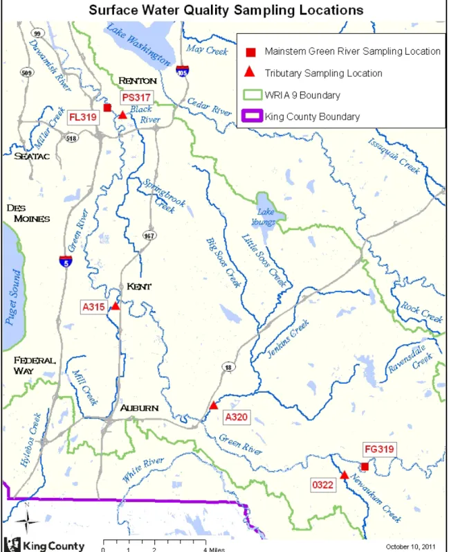
Figure 4. Sampling locations ...11
Tables
Table 1. Autosampler trigger heights above wet season baseflow for sampling in tributaries... 7Table 2. Green River and Tributary Sampling Locations and Locator Names... 9
Table 3. Number of Samples and Replicates per Sampling Locations ... 10
Table 4. Sample Container, Preservation, Storage, and Hold Time Requirements ... 14
Table 5. Labeled Surrogates and Recovery Standards Used for EPA Method 1668A PCB Congener Analysis ... 19
Table 6. PCB Congener water detection limit goals in pg/L and lower calibration limits by1668A, AXYS Analytical method MLA 010. ... 20
Table 7. PCBs QA/QC Frequency and Acceptance Criteria ... 24
Table 8. PAH Target Compounds and Detection Limit Goals in µg/L ... 25
Table 9. PAH QA/QC Frequency and Acceptance Criteria ... 26
Table 10. Arsenic Target Detection Limit Goals (µg/L) ... 26
Table 11. Arsenic QA/QC Frequency and Acceptance Criteria ... 27
Table 12. Conventionals Analytical Methods and Detection Limit Goals in mg/L ... 27
ACRONYMS
AXYS Analytical AXYS Analytical Services Ltd.
COC chain of custody
CSO combined sewer overflow
DOC dissolved organic carbon
DQOs data quality objectives
Ecology Washington Department of Ecology
EPA US Environmental Protection Agency
FSU Field Science Unit
KCEL King County Environmental Laboratory
LCS laboratory control sample
LDW Lower Duwamish Waterway
LIMS Laboratory Information Management System
LMCL lowest method calibration limits
LPAH low molecular weight PAHs
MDL method detection limit
ML minimum level
MRL method reporting limit
OPR ongoing precision and recovery
PAH polycyclic aromatic hydrocarbon
PCB polychlorinated biphenyls
RDL reporting detection limit
RPD relative percent difference
RI remedial investigation
PQL practical quantitation limit
QA/QC quality assurance/quality control
QC quality control
SAP sampling and analysis plan
SCWG Source Control Work Group
SDL specific detection limit
SS stainless steel
TOC total organic carbon
TSS total suspended solids
WLRD King County Water and Land Resources Division
1.0.
INTRODUCTION
This sampling and analysis plan (SAP) presents project information and sampling and analytical methodologies for the Green River Loading Study. These methods will be employed to collect whole surface water samples and flow measurements to better understand the relative
contribution of polychlorinated biphenyls (PCBs), polycyclic aromatic hydrocarbons (PAHs), and arsenic associated with suspended solids, to the Duwamish River from upstream areas in the Green River.
1.1
Project Background
The Duwamish River originates at the confluence of the Green and Black Rivers near Tukwila, Washington, and flows northwest for approximately 19 km (12 mi), splits at the southern end of Harbor Island to form the East and West Waterways, and then discharges into Elliott Bay in Puget Sound, Seattle, Washington. The Lower Duwamish Waterway (LDW) is approximately 5 miles long and consists of the downstream portion of the Duwamish River, excluding the East and West Waterways.
King County is a member of the Source Control Work Group (SCWG) for the Lower Duwamish Superfund site. Other members include lead agency Washington Department of Ecology
(Ecology), US Environmental Protection Agency (EPA), City of Seattle and the Port of Seattle. The SCWG works to understand potential chemical sources within the LDW Superfund site and to control and reduce sources that can contaminate waterway sediments. King County
Wastewater Treatment Division (WTD) seeks to better understand the potential sources of contaminants of concern into combined sewer overflow (CSO) basins which discharge to the LDW and also contaminant inputs to the LDW from upstream sources.
The LDW Remedial Investigation (RI) (Windward 2010) indicates that more than 99% of the new sediment deposited in the LDW each year originates upstream of the LDW in the
Green/Duwamish River basin. Because of this, LDW surface sediment quality will be closely tied to the quality of incoming sediment from the Green/Duwamish River. A number of studies and sampling programs have evaluated the water chemistry and the chemistry of the suspended solids from the Green/Duwamish River system (King County 2007; Gries and Sloan 2009; Windward 2010). While King County has conducted a number of sampling events to evaluate water quality in the Green/Duwamish River, a study that provides information regarding the relative contributions of PCBs, PAHs and arsenic has not been conducted by King County. The primary purpose of the sampling and analysis effort described here is to provide a better
understanding of the relative chemistry load of these contaminants from the major tributaries to the Green/Duwamish River and ultimately to the LDW to improve the understanding their inputs.
This study will focus on PCBs, PAHs, and arsenic because the LDW RI has identified these as human health contaminants of concern (COC) within the LDW and residual risks are predicted to be present after cleanup. Dioxins/furans were also identified as human health COC; however, these chemicals are not included in this study because they are not expected to be present at detectable levels in surface water samples.
1.2
Scope of Work
This sampling effort will involve collection and analysis of whole surface water samples for analysis of PCBs, PAHs and arsenic from two locations on the Green River and four tributaries that discharge to the river. The data collected by this effort will be used to estimate relative contributions of these chemicals from the major tributaries to the Green River and to the LDW. This study will not collect sufficient information to estimate total contaminant loading to the LDW. Samples will be collected during dry season baseflow (3 events) and wet season/storm flow (up to 6 events) conditions from these six locations. Locations include upper and lower boundary locations along the mainstem of the Green River, and four major tributaries: Soos Creek, Newaukum Creek, Mill Creek and the Black River. The upper boundary location on the Green River (upriver of the major tributaries to be sampled) will be the entrance bridge to Flaming Geyser State Park, while the lower boundary location on the Green River (downstream of the tributaries) will be at the Foster Links Golf Course in Tukwila. All samples will be analyzed for PCB congeners, PAHs, and arsenic in addition to total organic carbon (TOC), dissolved organic carbon (DOC) and total suspended solids (TSS). In addition, flow
measurements (or estimates in the case of the mainstem locations and the Black River Pump station) will be collected.
1.3
Survey Schedule
Field reconnaissance was conducted in March and April 2011 to evaluate feasible sampling locations in the Green River and at the major tributaries. Dry season baseflow samples will be collected in September 2011. Wet season/storm event samples will be collected between
October 2011 and March 2012. Analysis of samples is expected to continue through early 2012. It is anticipated that data from all sampling events will be validated, reviewed, and ready for release by the last quarter of 2012.
1.4
Project Staff
The following staff members are responsible for project execution:
Jeff Stern, LDW Project Manager ... 206-263-6447 Wastewater Treatment Division Manager and Technical lead for all
Lower Duwamish River studies.
Deb Lester, Green River Study Project Manager... 206-296-8325 Responsible for basin study project execution and adherence to SAP
and schedule.
Debra Williston, Water and Land Resources Division Technical Lead ... 206-263-6540 Technical Support for all Lower Duwamish River studies including
study project.
Responsible for sample collection.
Fritz Grothkopp, KC Environmental Lab Project Manager ... 206-684-2327 Manages sample analysis, sample shipment, and data delivery.
Scott Mickelson, Data Validation Lead ... 206-296-8247 Responsible for all data validation.
2.0.
STUDY DESIGN
The goal of this effort is to collect surface water samples and flow information that represent dry season base flow and wet weather/storm flow conditions in the major tributaries (Soos Creek, Newaukum Creek, Mill Creek and Black River) and at two locations in the Green River prior to and after input from the tributaries. All samples will be analyzed for PCB congeners, PAHs, arsenic, TSS, TOC and DOC. Resulting data will allow King County to begin to estimate relative contributions of these contaminants to the LDW from the Green River basin.
2.1
Data Quality Objectives
The data quality objectives (DQOs) for this project are to collect data of known and sufficient quality to meet the survey goals. Validation of project data will assess whether the data collected are of sufficient quality to meet the survey goals. The data quality issues of precision, accuracy, bias, representativeness, completeness, comparability, and sensitivity are described in the following sections, along with data validation. Data validation is discussed in Section 5.0.
2.1.1 Precision, Accuracy, and Bias
Precision is the agreement of a set of results among themselves and is a measure of the ability to reproduce a result. Accuracy is an estimate of the difference between the true value and the measured value. The accuracy of a result is affected by both systematic and random errors. Bias is a measure of the difference, due to a systematic factor, between an analytical result and the true value of an analyte. Precision, accuracy, and bias for analytical chemistry may be measured by one or more of the following quality control (QC) samples:
• Analysis of various laboratory QC samples such as method blanks, spiked blanks, matrix
spikes, laboratory control samples and laboratory duplicates or triplicates; and
• Collection and analysis of field replicate samples.
Precision of replicates is expected to be within the limits specified in Section 4. If precision is considered too low for project needs, these data will be used to guide future sampling efforts. Accuracy is assessed through matrix spikes and spike duplicates along with the ongoing
precision and recovery sample control charts. Additionally, the isotopic dilution method chosen for this study is the most rigorous method for PCB congener analysis. This method uses
isotopically-labeled congeners, to track the recovery performance of the range of congener homologs. Thus, each congener concentration is theoretically adjusted for the extraction efficiency and analytical performance of that specific sample.
2.1.2 Representativeness
Representativeness expresses the degree to which sample data accurately and precisely represent a characteristic of a population, parameter variations at the sampling point, or an environmental condition. Surface water samples will be collected from stream or river locations to represent water quality during defined flow conditions. The samples are intended to generate data of
sufficient quality to provide initial estimates of the contribution of PCBs, PAHs and arsenic from the major tributaries and the upper mainstem Green River to the LDW.
Samples are to be collected in such a manner as to minimize potential contamination and other types of degradation in the chemical and physical composition of the water. This can be achieved by following guidelines for sampler decontamination, sample acceptability criteria, sample processing, observing proper hold-times, preservation, storage and preparation of samples.
2.1.3 Completeness
Completeness is defined as the total number of samples analyzed for which acceptable analytical data are generated, compared to the total number of samples submitted for analysis. Sampling with adherence to standardized sampling and testing protocols will aid in providing a complete set of data for this survey. The goal for completeness is 90%. The samples from each event should produce greater than 90% acceptable data under the QC conditions described elsewhere in this SAP.
2.1.4 Comparability
Comparability is a qualitative parameter expressing the confidence with which one data set can be compared with another. This goal is achieved through the use of standard techniques to collect and analyze representative samples, along with standardized data validation and reporting procedures. By following the guidance of this SAP, the goal of comparability between this and future sampling events will be achieved. Where available, historical surface water data for the Green River and associated tributaries may be compared with data generated from this survey to enhance data analysis efforts. Previous data will be used if comparable sampling and/or
analytical techniques were employed. Previous sampling efforts have collected both flow weighted and grab surface water samples for analysis of conventional parameters and metals. However, PCB congeners and low level PAHs have not been analyzed in surface water samples from all of these locations, thus these data may have limited comparability to other King County data.
2.1.5 Sensitivity
Sensitivity is a measure of the capability of analytical methods to meet the survey goal. The analytical method detection limits presented in Section 5 are sensitive enough to detect PCB congeners, low level PAHs and arsenic at concentrations of interest to increase the understanding of the relative contribution of these chemicals to the Duwamish River from the Green River.
2.2
Sampling and Analytical Strategy
The sampling strategy is designed to provide data sufficient to provide initial estimates of the relative contribution of PCBs, PAHs and arsenic from the Green River and its major tributaries to the LDW. This study includes four major tributaries of the Green River, as well as two
locations on the Green River (up- and downstream of the tributary locations) to begin to evaluate relative inputs of PCBs, PAHs and arsenic on a finer scale (subbasins). The study is designed to address the following questions:
1) How do the relative contributions of PCBs, PAHs and arsenic differ during dry season baseflow and wet season/storm conditions?
2) What are initial estimates of the relative contributions of PCBs, PAHs and arsenic
from the major tributaries and the Green River to the LDW?
To answer these questions, autosamplers and flow measuring equipment will be used to collect composite samples from the six locations during both dry season baseflow and wet season/storm conditions. The upper boundary sampling location in the Green River is located upstream of the Newaukum Creek confluence at Flaming Geyser State Park; while the downstream boundary location is adjacent to Foster Links Golf Course in Tukwila. The four tributary locations are located on Mill, Newaukum, and Soos Creeks and at the outflow of the Black River Pump Station.
Baseflow Sample Collection
Three sets of samples will be collected from the six locations during dry season baseflow conditions; dry season is defined as May through beginning of October. All baseflow samples will be time weighted composites conducted during September 2011 with an antecedent dry period of at least 3 days.
Because flow is not expected to vary substantially during baseflow conditions, time weighted composite samples, rather than flow weighted composite samples, will be collected. Dry season baseflow samples will be collected from the Black River Pump Station when the electric
baseflow pump is the only pump running.
Flow during baseflow sample collection at Newaukum and Soos Creeks and the mainstem Green River locations will be based on US Geological Survey (USGS) gage data for the time period when samples are collected. Flow at the Green River mainstem locations will be estimated, based on flow from USGS gage at Auburn, WA (Gage 12113000). Current gage data are not available for the Mill Creek sampling location. Flow at the Mill Creek site will be manually measured using a Swoffer flow meter just prior to sample collection and again when sample collection is complete. Flow is not expected to vary significantly during collection of baseflow samples; therefore flow meters will not be used during sample collection. Flow at the Black River pump station will be estimated based on the pumping rate at the time of sampling.
Tributary Storm/Wet Season Sample Collection
Tributary storm event sample collection from three of the tributary locations (Soos, Mill and Newaukum Creeks) will be triggered by wet season flows/storm events; wet season is defined as October through April. Six sets of samples will be collected from these tributaries during storm/wet season conditions. Autosamplers will be triggered to initiate sampling at a specific stage height above the current wet season baseflow. Trigger heights above wet season baseflow will be such that a storm of approximately 0.25 to 0.5” in 12 hours (with a 24 hour antecedent dry period) should be sufficient to trigger sampling, however, less intense but longer duration storms may also initiate autosampling. Existing rain gages will be used to describe the relative intensity of the storms which raised flow sufficiently to trigger autosampling.
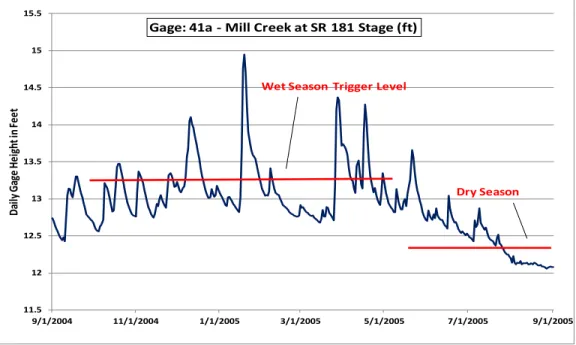
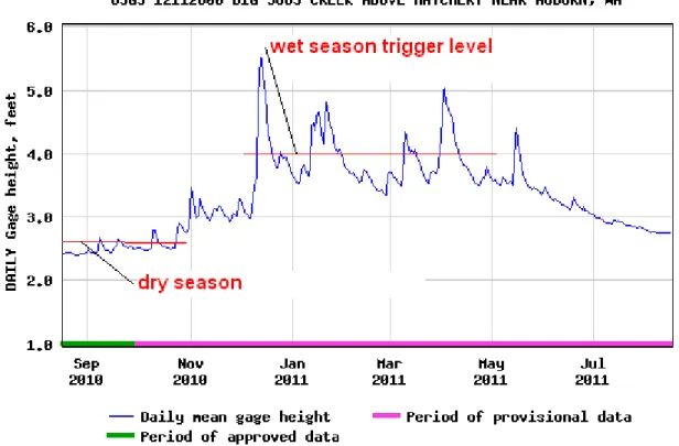
After triggering, samplers will collect flow weighted composites for the next 12–24 hours (a maximum of 24 hours). Table 1 shows the autosampler trigger heights, while Figures 1, 2 and 3
illustrate the seasonal hydrographs and trigger heights based on their respective seasonal baseflow conditions. Trigger heights were established based on historic flow regimes such that six wet season storm flows at each location were likely to be sampled. The intent is to capture wash-off events with the highest potential to transport target chemicals downstream. Note that trigger heights are not absolute elevations; for practical reasons they are measured above the current base flow to account for year to year variation. There is evidence that backwater
conditions occur in Mill Creek in the vicinity of the sampling location. As sampling progresses, the sampling protocol at this location may need to be revaluated; any changes will be
documented in the data report. Figures 1, 2, and 3 are provided to illustrate the magnitude of stage change during historic storm events. The trigger heights shown in Table 1 may be revised if weather patterns or flow regimes in the 2011–2012 water year appear to be significantly different. During sample collection, continuous flow will be directly measured in Soos, Newaukum, and Mill creeks using ISCO flow meters.
Table 1. Autosampler tr igger heights above wet season baseflow for sampling in
tr ibutar ies.
Tributary Location Trigger Height
Mill Creek 5”
Soos Creek 6”
Newaukum Creek 4”
Note: Heights estimated from flow records shown in Figures 1, 2, and 3.
Figur e 1. Mill Cr eek histor ic flow r ecor d with estimated sampling tr igger height for wet
season sampling. 11.5 12 12.5 13 13.5 14 14.5 15 15.5 9/1/2004 11/1/2004 1/1/2005 3/1/2005 5/1/2005 7/1/2005 9/1/2005 Da ily G ag e H ei gh t i n F ee t
Gage: 41a - Mill Creek at SR 181 Stage (ft)
Wet Season Trigger Level
Figur e 2. Big Soos histor ic flow r ecor d with estimated sampling tr igger height for wet season sampling.
Figur e 3. Newaukum cr eek histor ic flow r ecor d with estimated sampling tr igger height
Mainstem Green River Storm/Wet Season Sample Collection
Six storm event samples will also be collected from the two Green River mainstem locations; sampling will be triggered by specific rainfall conditions; at least 0.25 inch of rain with a minimum 24 hour antecedent dry period. If possible, at least 3 of the 6 samples will be targeted
for collection when the Howard Hansen Dam is not releasing a significant volume (Oct < 250
cfs; Nov < 500 cfs; Dec < 600; Jan - April < 700 cfs) of water to the Green River. Samples from the Green River mainstem sampling locations will be 24 hour time weighted composites. Flow at the mainstem Green River sampling locations will be estimated using data from the USGS gage at Auburn WA (Gage 12113000).
Black River Pump Station Storm/Wet Season Sample Collection
Six event samples targeting two flow regimes will be collected at the outlet of the Black River pump station; “moderate stormflow condition” sampling will be triggered by a storm event that results in at least one additional pump operating at the pump station in addition to the small electric baseflow pump. “Large stormflow” will be triggered when the pump station is using 2 or more extra pumps to evacuate larger water volumes. There is likely to be a variable lag time between the actual storm event and initiation of additional pumping at the site. Samples from the Black River Pump station will be 24 hour time weighted composites. Flow at the Black River Pump station will be estimated using pumping rate data based on pump station operations.
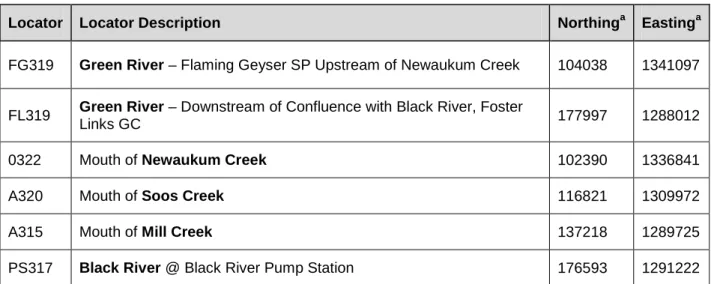
2.2.1 Sampling Station Locations and Sample Identification
Sample locations will be identified using a unique locator name. The locator name, the date of collection and the unique sample identification number generated by King County
Environmental Laboratory (KCEL) will identify individual samples collected at each location. The six sampling locations are shown in Figure 4. The corresponding locator numbers and sample coordinates are shown in Table 2.
Table 2. Gr een River and Tr ibutar y Sampling Locations and Locator Names.
Locator Locator Description Northinga Eastinga
FG319 Green River – Flaming Geyser SP Upstream of Newaukum Creek 104038 1341097
FL319 Green River – Downstream of Confluence with Black River, Foster
Links GC 177997 1288012
0322 Mouth of Newaukum Creek 102390 1336841
A320 Mouth of Soos Creek 116821 1309972
A315 Mouth of Mill Creek 137218 1289725
PS317 Black River @ Black River Pump Station 176593 1291222
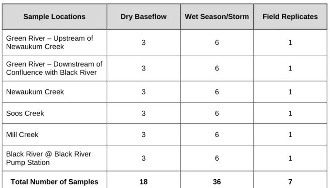
2.2.2 Sample Acquisition and Analytical Parameters
King County Field Science Unit (FSU) staff will primarily conduct sampling; however, other King County Water and Land Resources staff may provide assistance as needed. Sampling techniques are discussed in Section 3. Each sample will be analyzed for 209 PCB congeners, low level PAHs and arsenic along with DOC, TOC, and TSS. Table 3 summarizes the number of samples to be collected at each location including estimated number of sample replicates. The specific PAHs are listed in Section 4. PCB congener analysis will be conducted by AXYS Analytical in Sidney, British Columbia. All other chemical analyses and conventional analyses will be conducted by the KCEL, a Washington State Department of Ecology Certified
Laboratory.
Table 3. Number of Samples and Replicates per Sampling Locations
Sample Locations Dry Baseflow Wet Season/Storm Field Replicates
Green River – Upstream of
Newaukum Creek 3 6 1
Green River – Downstream of
Confluence with Black River 3 6 1
Newaukum Creek 3 6 1
Soos Creek 3 6 1
Mill Creek 3 6 1
Black River @ Black River
Pump Station 3 6 1
Total Number of Samples 18 36 7
Note: one equipment blank will be collected at the downstream mainstream Green River location over the course of the sampling period (see Section 3.7).
3.0.
SAMPLING PROCEDURES
This section describes field procedures that will be used to collect the samples. Procedures are described for collecting samples including equipment used, decontaminating sampling
equipment, and recording field measurements and conditions. Requirements for sample containers and preservation, and sample custody procedures are also described.
3.1
Sample Collection
Composite water quality samples will be collected using ISCO autosamplers equipped with 10-liter glass carboys. Auto samplers will be fitted with a minimum of new and pre-cleaned silicon tubing in the peristaltic pump for each sampling event. Teflon® tubing and stainless steel (SS) fittings shall be used for all other tubing runs. Teflon tubing will be dedicated to a sampling location. Autosamplers will be secured at monitoring sites in locked housings or utility boxes (or
other suitable option). A target amount of five-seven liters of water will be collected over the
course of each sampled event.
For all dry season baseflow samples and all mainstem Green River and Black River pump station samples, time-weighted samples will be collected. The auto samplers will be set to automatically trigger sample collection at 30 minute time intervals at each location. The total time of
collection will not exceed 24 hours. Conditions for these sampling events are discussed in Section 2.2.
For wet season/storm samples at Soos, Mill and Newaukum Creeks, flow-weighted samples will be collected. A flow meter will be installed and continuous flow data will be recorded.
Triggering of autosampler for collection of flow weighted samples from Soos, Mill and Newaukum Creeks will be based on change in stage height and continue on a flow weighted basis for a maximum of 24 hours. An ISCO meter will be used to track flow at the three tributary locations. After a pre-determined volume of water passes by the autosampling
equipment, a pulse trigger is sent to the autosampler to collect a designated aliquot; the specific volume is estimated by FSU staff based on the forecasted intensity and duration of the storm. Samples will be collected over a maximum of 24 hours with a goal of collecting at least 8 and no more than 10 liters.
As soon as possible following the sampling event, FSU staff will retrieve the sample carboy and place it in a cooler with ice for transport to KCEL. The composite sample will then be
transferred into the appropriate laboratory sample containers. This will be done by continuously agitating the sample in the carboy while transferring sample aliquots to the appropriate
laboratory containers using a Teflon® siphon tube. Each sample container will be filled to the appropriate level from the autosampler carboy. This procedure will ensure a representative sample from the carboy in each laboratory sample container. Once the sample has been split, the dissolved arsenic sample will be filtered. Dissolved arsenic samples will be drawn through a cleaned Nalgene 500 mL filtration apparatus with a 0.45 micron filter using a peristaltic pump. Because the sample aliquot for dissolved arsenic cannot be filtered within 15 minutes of collection, appropriate hold-time violation flags will be added to the data.
3.2
Sampling Equipment
In addition to the samplers discussed in Section 3.1, the field equipment listed below will be available for field staff.
1) Sampling supplies:
a) Cooler with ice
b) Nitrile gloves
2) Safety equipment:
a) Hard hat
b) Safety vest
c) Safety shoes and glasses
d) Appropriate traffic control equipment and personnel where applicable (FSU supervisor
will approve safety plan)
e) Documentation supplies:
f) Field notebook
g) Sample labels
h) Chain-of-custody forms
i) Camera
When visiting the sampling station, field personnel will record the following information on field forms that are maintained in a waterproof field notebook.
• Date
• Time of sample collection or visit
• Name(s) of sampling personnel
• Description of sampling location (e.g., closest street intersection)
• Weather conditions
• Number and type of samples collected
• Field measurements
• Log of photographs taken, if any taken
• Comments on the working condition of the sampling equipment
• Deviations from sampling procedures
• Unusual conditions (e.g., water color or turbidity, presence of oil sheen, odors, and land
disturbances)
3.3
Equipment Decontamination
Once samples are collected, all re-usable equipment should be decontaminated. New Teflon®
a deionized water (ASTM I or II) rinse1; all tubing will be dedicated to a specific site. Glass (or Teflon) carboys will be cleaned in the following manner: (1) Detergent 8 laboratory detergent
followed with a hot water rinse; (2) soaked in or rinsed with a 5% sulfuric acidsolution rinse; (3)
a deionized water (ASTM I or II) rinse; and (4) an acetone rinse. All SS fittings and connectors are cleaned in the same manner with the exception of the acid rinse step. Composite autosampler carboys and autosampler tubing will be cleaned prior to each sampling event according to
laboratory standard operating procedures (KCEL SOP # 234v1 and KCEL SOP #223v2) for collecting samples for low-level analysis using autosamplers. Acetone solvent rinses shall be used for glass carboys per EPA method 1668a. Proofed clean PCB sampling containers will be supplied by AXYS Analytical. One equipment blank will be analyzed to check for possible cross contamination between sampling events. Proper personal protective equipment (new powder-free gloves) will be worn during sampling activities and during decontamination
processes.
3.4
Sample Delivery and Storage
All samples (in autosampler carboys) will be kept in ice-filled coolers until delivery to the KCEL, on the same day that they were collected. Because auto samplers will automatically initiate sampling, samples cannot be refrigerated during the compositing process. Additional sample preservation, if required, will be performed upon receipt of the samples at the KCEL. Samples will be split from the glass auto-sampler container into the appropriate analytical containers and preserved according to method specifications at the KCEL.
Containers for PCB congener analysis will be delivered to AXYS Analytical within 1 to 3 months of sample collection. Samples will be held at KCEL at the appropriate temperature until delivery date. Samples will be maintained in coolers with ice and/or ice packs during the delivery process. Samples will either be driven to AXYS Analytical or shipped via overnight express delivery service. Table 4 shows sample handling and storage requirements.
Table 4. Sample Container , Pr eser vation, Stor age, and Hold Time Requir ements
Analyte Container Preservation Storage Hold Time
PCB Congeners 2 x 1-L amber
glass None
refrigerate at 4oC
in the dark 1 year
Total Organic Carbon
2 x 40-mL amber glass VOA
H3PO4 to pH<2
within 1 day refrigerate at <6 o
C 28 days
Dissolved Organic Carbon
125 mL amber wide mouth HDPE
0.45 µm filtration, then H3PO4 to pH<2 within 1 day
refrigerate at <6oC 28 days
1 Acetone will not be used to clean Teflon or silicone tubing used for sample collection due to interference (false
Analyte Container Preservation Storage Hold Time
Total Suspended Solids
1-L clear wide
mouth HDPE None refrigerate at <6
o
C 7 days
PAHs 2 x 1L amber
glass None refrigerate at 4
o
C 7/401
Arsenic (Total & Dissolved) 500 mL Acid washed HDPE ultra-pure HNO3 to pH<2 n/a 180 days 2
1 7 days from sampling to extraction, 40 days from extraction to analysis 2
Within 15 minutes of collection, dissolved metals samples must be filtered (.45 µm).
3.5
Chain of Custody
Chain of custody (COC) will commence at the time that each autosampler is deployed. The autosampler will be secured to ensure no tampering has occurred and all samples will be under direct possession and control of King County field staff or locked in a controlled area. For COC purposes, locked field sheds, autosamplers and field vehicles will be considered “controlled areas.” All sample information will be recorded on a COC form (Appendix A). This form will be completed in the field and will accompany all samples during transport and delivery to the laboratory. Upon arrival at the KCEL, the samples will be split in the appropriate containers then relinquished to the sample login person. The date and time of sample delivery will be recorded and both parties will then sign off in the appropriate sections on the COC form at this time. Once completed, original COC forms will be archived in the project file.
Samples delivered after regular business hours will be stored in a secure refrigerator until the next day. Samples delivered to AXYS Analytical will be accompanied by a properly-completed KCEL COC form and custody seals will be placed on the shipping cooler. AXYS Analytical will be expected to provide a copy of the completed COC form as part of their analytical data package.
3.6
Sample Documentation
Sampling information and sample metadata will be documented using the methods noted below.
• Field sheets generated by King County’s Laboratory Information Management System
(LIMS) will be used at all stations and will include the following information:
1. Sample ID number
2. Location name
3. Start-end stage heights and times
4. Date and time of sample collection (start and end times of the compositing period)
5. Initials of all sampling personnel
• LIMS-generated container labels will identify each container with a unique sample
• The field sheet will contain records of collection times, general weather and the names of field crew staff.
• COC documentation will consist of KCEL’s standard COC form, which is used to track
release and receipt of each sample from collection to arrival at the lab.
3.7
Field Replicates and Equipment Blanks
Field replicates will be collected using a separate additional auto sampler rotated between the sampling stations; one replicate will be collected from each station over the course of the study for a total of 6 replicates. Field replicates will be analyzed for all parameters. Field replicates will provide a measure of variability at sampling locations.
Collection and analysis of one equipment blank at the lower Green River mainstem sampling location (Site FL319) will be required for one sampling event. The analysis of the equipment blank will be used to evaluate levels of contamination that might be associated with the sampling equipment and introduce bias into the sample result. An aliquot of a clean reference matrix (reverse osmosis water) will be processed through the sampling equipment as a blank and analyzed for PCB congeners, PAHs, DOC, TOC and arsenic. The following conditions apply to collection of the equipment blank sample:
• The equipment blank sample must be collected with the same tubing and sampling
apparatus to be used to collect the samples.
• The equipment blank sample will be collected before the sampling begins.
As with the regular samples, the carboy with the equipment blank sample must be returned to KCEL for transfer of contents into the appropriate sample bottles. Equipment blanks shall be preserved, stored, and analyzed in the same manner as environmental samples. Field blank results for PCB congeners should be consistent with the blank criteria in sections 4.1. For PAHs and arsenic, field blank results should be <MDL.
4.0.
ANALYTICAL METHODS AND
DETECTION LIMITS
Analytical methods are presented in this section, along with analyte-specific detection limit goals. For the PAHs, arsenic and selected conventional analytes, the terms MDL and RDL, used in the following subsections, refer to method detection limit and reporting detection limit,
respectively. The KCEL reports both the LIMS reporting detection limit (LIMS RDL) and the LIMS method detection limit (LIMS MDL) for each sample and parameter, where applicable. EPA’s Office of Wastewater generally defines the PQL (practical quantitation limit) as the minimum concentration of a chemical constituent that can be reliably quantified, while the MDL is defined as the minimum concentration of a chemical constituent that can be detected. The KCEL LIMS RDL is analogous to the PQL for all analyses. It is verified either by including it on the calibration curve or by running a low level standard near the PQL value during the analytical run.
For arsenic and conventionals analyses, LIMS MDLs are typically two to five times higher than the statistically derived MDLs that are calculated by the 40 CFR Part 136, Appendix B procedure (Federal Register, Appendix B. 2007). In the case of some conventionals tests, MDLs are
evaluated by the procedure listed inappendix of 40 CFR Part 1362
Actual KCEL MDLs and RDLs may differ from the target detection limit goals as a result of necessary analytical dilutions or a reduction of extracted sample amounts based upon available sample volumes. Every effort will be made to meet the MDL/RDL goals listed in the SAP.
. The detection limits derived from this approach are also typically two to five times the statistically derived MDLs that are calculated by the 40 CFR Part 136, Appendix B procedure. In the case of organic mass spectral analyses (i.e., for PAHs), a standard analyzed near the MDL concentration during calibration must produce a valid mass spectra and this standard is used to define the MDL.
For PCB high resolution isotopic dilution based methods, the MDL and RDL terms are less applicable because limits of quantitation are derived from calibration capabilities and ubiquitous, but typically low level equipment and laboratory blank contamination. Additional reporting limit terms used particularly for PCB congener analyses are sample specific detection limits and lowest method calibration limits. Sample specific detection limit (SDL) is determined by converting the area equivalent to 2.5 times the estimated chromatographic noise height to a concentration. SDLs are determined individually for every congener, of each sample analysis run and accounts for any effect of matrix on the detection system and for recovery achieved through the analytical work-up. Lowest method calibration limits (LMCL) are based on calibration points from standard solutions. They are prorated by sample size and are supported by statistically-derived method reporting limit (MRL) values.
2 Appendix D: DQ FAC Single Laboratory Procedure v2.4 of the Federal Advisory Committee on Detection and
The PCB congener data will be reported to LMCLs and flagged down to the SDL value. In many cases the SDL may be below the LMCL. Method 1668A defines a Minimum Level (ML) value for each congener. The ML value is used to evaluate levels in the method blank. The ML is based on the lowest method calibration limit (LMCL) and any laboratory performing the method should be able to achieve at least that level. AXYS Analytical uses an additional
calibration point that is lower than the calibration points specified in the method; as such they are able to quantify congeners below the ML specified in the method.
Details regarding the frequency of required QC samples are provided in the individual analytical sections shown below. In general for all methods, this frequency is 1 in 20 samples or 1 per batch whichever is more frequent. Below are general descriptions of types of laboratory QC samples:
• Analysis of method blanks is used to evaluate the levels of contamination that might be
associated with the processing and analysis of samples in the laboratory and introduce bias into the sample result. Method blank results for all target analytes (other than PCB congeners) should be “less than the MDL.”
• A laboratory duplicate is a second aliquot of a sample, processed concurrently and in an
identical manner with the original sample. The laboratory duplicate is processed through the entire analytical procedure along with the original sample in the same quality control batch. Laboratory duplicate results are used to assess the precision of the analytical method and the relative percent difference (RPD) between the results should be within method-specified or performance-based quality control limits. In the case of PAHs a matrix spike duplicate may be used in lieu of a laboratory duplicate due to the large number of non-detects frequently encountered in these analyses.
• A spike blank is a spiked aliquot of clean reference matrix used for the method blank.
The spiked aliquot is processed through the entire analytical procedure. Analysis of the spike blank is used as an indicator of method accuracy. It may be conducted in lieu of a laboratory control sample (LCS/SRM). A spike blank duplicate should be analyzed whenever there is insufficient sample volume to include a sample duplicate or matrix spike duplicate in the batch.
• The ongoing precision and recovery (OPR) samples must show acceptable recoveries,
according to the respective methods for data to be reported without qualification. The OPR sample is typically called a Lab Control Sample (LCS) or Spiked Blank in LIMS.
4.1
PCB Congeners
PCB congener analysis will follow EPA Method 1668A Revision A (EPA 2003), which is a high-resolution gas chromatography/high-resolution mass spectroscopy (HRGC/HRMS) method using an isotope dilution internal standard quantification. This method provides reliable analyte identification and very low detection limits. AXYS Analytical may be switching to Revision C of Method 1668 sometime during this project, depending on when EPA promulgates this revision. The principle differences between Method 1668A and 1668C are the replacement of individual laboratory acceptance criteria with inter-laboratory developed acceptance criteria. This change is not anticipated to modify result values, although there may be minor differences in data qualifiers not affecting usability. An extensive suite of labeled surrogate standards
(Table 5) is added before samples are extracted. Data are “recovery-corrected” for losses in extraction and clean-up, and analytes are quantified against their labeled analogues.
AXYS Analytical will perform this analysis according to their SOP MLA-010 Analytical Method for the Determination of 209 PCB Congeners by EPA Method 1668, which is a
proprietary document. A one-liter sample will be extracted followed by standard method clean-up, which includes layered Acid/Base Silica, Florisil and Alumina. Analysis is performed with an SPB Octyl column and a secondary DB1 column is used to resolve the co-eluting congeners PCB156 and PCB157. Method 1668A requires that if a sample contains more than 1% total solids, the solids and liquid will be extracted and analyzed separately.
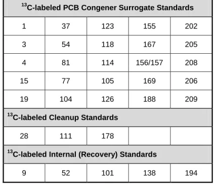
Table 5. Labeled Sur r ogates and Recover y Standar ds Used for EPA Method 1668A
PCB Congener Analysis
13
C-labeled PCB Congener Surrogate Standards
1 37 123 155 202 3 54 118 167 205 4 81 114 156/157 208 15 77 105 169 206 19 104 126 188 209 13
C-labeled Cleanup Standards
28 111 178
13
C-labeled Internal (Recovery) Standards
9 52 101 138 194
Table 6 lists the 209 PCB congeners and their respective target SDL and LMCL values. The reporting limits for individual samples may differ from those in Table 6 since they are determined by signal to noise ratios and changes to final volumes. Typical sample detection limits are shown. Note that several of the congeners co-elute and a single SDL or LMCL value is provided for the congeners in aggregate.
Table 6. PCB Congener water detection limit goals in pg/L and lower calibr ation limits by1668A, AXYS Analytical method MLA 010.
PCB Congener Typical Detection
Limit/MDL LMCL based on Low Cal./RDL CL1-PCB-1 1.0 4.0 CL1-PCB-2 1.0 4.0 CL1-PCB-3 1.0 4.0 CL2-PCB-4 2.0 4.0 CL2-PCB-5 2.0 4.0 CL2-PCB-6 2.0 4.0 CL2-PCB-7 2.0 4.0 CL2-PCB-8 2.0 4.0 CL2-PCB-9 2.0 4.0 CL2-PCB-10 2.0 4.0 CL2-PCB-11 2.0 4.0 CL2-PCB-12/13 2.0 8.0 CL2-PCB-14 2.0 4.0 CL2-PCB-15 2.0 4.0 CL3-PCB-16 1.0 4.0 CL3-PCB-17 1.0 4.0 CL3-PCB-19 1.0 4.0 CL3-PCB-21/33 1.0 8.0 CL3-PCB-22 1.0 4.0 CL3-PCB-23 1.0 4.0 CL3-PCB-24 1.0 4.0 CL3-PCB-25 1.0 4.0 CL3-PCB-26/29 1.0 8.0 CL3-PCB-27 1.0 4.0 CL3-PCB-28/20 1.0 8.0 CL3-PCB-30/18 1.0 8.0 CL3-PCB-31 1.0 4.0 CL3-PCB-32 1.0 4.0 CL3-PCB-34 1.0 4.0 CL3-PCB-35 1.0 4.0 CL3-PCB-36 1.0 4.0 CL3-PCB-37 1.0 4.0 CL3-PCB-38 1.0 4.0 CL3-PCB-39 1.0 4.0 CL4-PCB-41/40/71 1.0 12.0 CL4-PCB-42 1.0 4.0 CL4-PCB-43 1.0 4.0
PCB Congener Typical Detection Limit/MDL LMCL based on Low Cal./RDL CL4-PCB-44/47/65 1.0 12.0 CL4-PCB-45/51 1.0 8.0 CL4-PCB-46 1.0 4.0 CL4-PCB-48 1.0 4.0 CL4-PCB-50/53 1.0 8.0 CL4-PCB-52 1.0 4.0 CL4-PCB-54 1.0 4.0 CL4-PCB-55 1.0 4.0 CL4-PCB-56 1.0 4.0 CL4-PCB-57 1.0 4.0 CL4-PCB-58 1.0 4.0 CL4-PCB-59/62/75 1.0 12.0 CL4-PCB-60 1.0 4.0 CL4-PCB-61/70/74/76 1.0 16.0 CL4-PCB-63 1.0 4.0 CL4-PCB-64 1.0 4.0 CL4-PCB-66 1.0 4.0 CL4-PCB-67 1.0 4.0 CL4-PCB-68 1.0 4.0 CL4-PCB-69/49 1.0 8.0 CL4-PCB-72 1.0 4.0 CL4-PCB-73 1.0 4.0 CL4-PCB-77 1.0 4.0 CL4-PCB-78 1.0 4.0 CL4-PCB-79 1.0 4.0 CL4-PCB-80 1.0 4.0 CL4-PCB-81 1.0 4.0 CL5-PCB-82 1.0 4.0 CL5-PCB-83/99 1.0 8.0 CL5-PCB-84 1.0 4.0 CL5-PCB-88/91 1.0 8.0 CL5-PCB-89 1.0 4.0 CL5-PCB-92 1.0 4.0 CL5-PCB-94 1.0 4.0 CL5-PCB-95/100/93/102/98 1.0 20.0 CL5-PCB-96 1.0 4.0 CL5-PCB-103 1.0 4.0 CL5-PCB-104 1.0 4.0 CL5-PCB-105 1.0 4.0
PCB Congener Typical Detection Limit/MDL LMCL based on Low Cal./RDL CL5-PCB-106 1.0 4.0 CL5-PCB-107/124 1.0 8.0 CL5-PCB-108/119/86/97/125/87 1.0 24.0 CL5-PCB-109 1.0 4.0 CL5-PCB-110/115 1.0 8.0 CL5-PCB-111 1.0 4.0 CL5-PCB-112 1.0 4.0 CL5-PCB-113/90/101 1.0 12.0 CL5-PCB-114 1.0 4.0 CL5-PCB-117/116/85 1.0 12.0 CL5-PCB-118 1.0 4.0 CL5-PCB-120 1.0 4.0 CL5-PCB-121 1.0 4.0 CL5-PCB-122 1.0 4.0 CL5-PCB-123 1.0 4.0 CL5-PCB-126 1.0 4.0 CL5-PCB-127 1.0 4.0 CL6-PCB-128/166 1.0 8.0 CL6-PCB-130 1.0 4.0 CL6-PCB-131 1.0 4.0 CL6-PCB-132 1.0 4.0 CL6-PCB-133 1.0 4.0 CL6-PCB-134/143 1.0 8.0 CL6-PCB-136 1.0 4.0 CL6-PCB-137 1.0 4.0 CL6-PCB-138/163/129/160 1.0 16.0 CL6-PCB-139/140 1.0 8.0 CL6-PCB-141 1.0 4.0 CL6-PCB-142 1.0 4.0 CL6-PCB-144 1.0 4.0 CL6-PCB-145 1.0 4.0 CL6-PCB-146 1.0 4.0 CL6-PCB-147/149 1.0 8.0 CL6-PCB-148 1.0 4.0 CL6-PCB-150 1.0 4.0 CL6-PCB-151/135/154 1.0 12.0 CL6-PCB-152 1.0 4.0 CL6-PCB-153/168 1.0 8.0 CL6-PCB-155 1.0 4.0
PCB Congener Typical Detection Limit/MDL LMCL based on Low Cal./RDL CL6-PCB-156/157 1.0 8.0 CL6-PCB-158 1.0 4.0 CL6-PCB-159 1.0 4.0 CL6-PCB-161 1.0 4.0 CL6-PCB-162 1.0 4.0 CL6-PCB-164 1.0 4.0 CL6-PCB-165 1.0 4.0 CL6-PCB-167 1.0 4.0 CL6-PCB-169 1.0 4.0 CL7-PCB-170 1.0 4.0 CL7-PCB-171/173 1.0 8.0 CL7-PCB-172 1.0 4.0 CL7-PCB-174 1.0 4.0 CL7-PCB-175 1.0 4.0 CL7-PCB-176 1.0 4.0 CL7-PCB-177 1.0 4.0 CL7-PCB-178 1.0 4.0 CL7-PCB-179 1.0 4.0 CL7-PCB-180/193 1.0 8.0 CL7-PCB-181 1.0 4.0 CL7-PCB-182 1.0 4.0 CL7-PCB-183/185 1.0 8.0 CL7-PCB-184 1.0 4.0 CL7-PCB-186 1.0 4.0 CL7-PCB-187 1.0 4.0 CL7-PCB-188 1.0 4.0 CL7-PCB-189 1.0 4.0 CL7-PCB-190 1.0 4.0 CL7-PCB-191 1.0 4.0 CL7-PCB-192 1.0 4.0 CL8-PCB-194 1.0 4.0 CL8-PCB-195 1.0 4.0 CL8-PCB-196 1.0 4.0 CL8-PCB-197/200 1.0 8.0 CL8-PCB-198/199 1.0 8.0 CL8-PCB-201 1.0 4.0 CL8-PCB-202 1.0 4.0 CL8-PCB-203 1.0 4.0 CL8-PCB-204 1.0 4.0
PCB Congener Typical Detection Limit/MDL LMCL based on Low Cal./RDL CL8-PCB-205 1.0 4.0 CL9-PCB-206 1.0 4.0 CL9-PCB-207 1.0 4.0 CL9-PCB-208 1.0 4.0 CL10-PCB-209 1.0 4.0
SDL = sample detection limit
LMCL = lower method calibration limit pg/L = picograms per liter
Quality control samples include method blank, OPR sample, and surrogate spikes. Method blanks and OPR, which are the same as spike blanks, are each included with each batch of samples. Surrogate spikes are labeled compounds that are included with each sample. The sample results are corrected for the recoveries associated with these surrogate spikes as part of the isotope dilution method. In addition, a laboratory duplicate will be conducted with each batch of samples. Note that a matrix spike and matrix spike duplicate are not required, nor meaningful under Method 1668A. Method 1668A has specific requirements for method blanks that must be met before sample data can be reported (see section 9.5.2 of Method 1668A). The OPR samples must show acceptable recoveries, according to Method 1668A, in order to samples to be analyzed and data to be reported. A summary of the quality control samples are shown in Table 7.
Table 7. PCBs QA/QC Fr equency and Acceptance Cr iter ia
Frequency Method Blank Lab Duplicate
(RPD)
OPR (% Recovery)
Surrogate Spikes
1 per batch* 1 per batch* 1 per batch* Each sample
PCB Congeners <LMCLa RPD <50% laboratory
QC limits b
laboratory QC limits b
batch = 20 samples or less prepared as a set
a
EPA Method 1668A blank criteria (see Table 2 of the published method) is to be below the Minimum Levels: 2, 10, 50 pg/congener depending on the congener with the sum of all congeners below 300 pg/sample. Higher levels are acceptable when sample concentrations exceed 10x the blank levels.
b
The laboratory’s performance-based control limits that are in effect at the time of analysis will be used as quality control limits. LMCL = Lowest Method Calibration Limit
RPD = Relative Percent Difference OPR = ongoing precision and recovery
4.2
Polycyclic Aromatic Hydrocarbons (PAHs)
Samples will be analyzed for the PAHs included in Table 8 below. The samples will be prepared by liquid-liquid extraction as detailed in method EPA method 3520C, KCEL SOP 701. Samples will be analyzed according to EPA Method 8270D; Gas Chromatography/Mass Spectrometry with Selected Ion Monitoring and Large Volume Injection method (GC/MS-SIM LVI). An SOP is currently being developed for this project. MDL and RDL goals are based upon extraction of one-liter of sample concentrated to 1.0 ml final volume. Depending upon the matrix, additional cleanups may be performed to ensure adequate instrument performance.
Every effort will be made to meet the target MDL and RDL goals. Due to the challenges of reporting as many detectable compounds as possible, there may need to be a change to the sample volumes, concentration factors or employ additional cleanups if the analytical protocols in the SOP do not yield enough detectable analytes to meet the project DQOs. Prior to
implementing a method changes, the project manager will be consulted and method change will undergo a project level review.
In addition to reporting individual PAH results, KCEL will report total high molecular weight PAHs (HPAHs) and total low molecular weight PAHs (LPAHs) as the sum of detected HPAHs
or LPAHs, respectively3. If no PAHs are detected within the LPAH or HPAH class, the reported
MDL/RDL for these totals will be the highest MDL/RDL reported for the individual PAHs in that class. When individual PAHs in HPAH or LPAH are detected, the reported MDL/RDL for these totals will be the lowest MDL/RDL from the respective LPAH or HPAH class.
Table 8. PAH Tar get Compounds and Detection Limit Goals in µg/L
Analyte MDL RDL Analyte MDL RDL 2-Methylnaphthalene 0.0010 0.0200 Chrysene 0.00025 0.00125 Acenaphthene 0.0010 0.00500 Dibenzo(a,h)anthracene 0.00050 0.00250 Acenaphthylene 0.0010 0.00500 Fluoranthene 0.00065 0.00650 Anthracene 0.00050 0.00250 Fluorene 0.0011 0.00550 Benzo(a)anthracene 0.00050 0.00250 Indeno(1,2,3-cd)Pyrene 0.00025 0.00125 Benzo(a)pyrene 0.00025 0.00125 Naphthalene 0.0010 0.0400 Benzo(b,j,k)fluoranthene 0.00050 0.00500 Phenanthrene 0.0010 0.0100 Benzo(g,h,i)perylene 0.00025 0.00125 Pyrene 0.00050 0.00500
NOTE: The MDL/RDL limits are calculated on a 1 liter extraction to a final volume of 1 ml. MDL/RDL limits will vary depending on amount extracted and final volume.
In addition to the surrogates and internal standards, which assess sample accuracy and bias, a method blank, spike blank, matrix spike and matrix spike duplicate or laboratory duplicate will be analyzed with each set of 20 samples, or one per QC batch. Matrix spike and matrix spike duplicate samples will only be prepared when sufficient water volumes are available. QA/QC frequency and acceptance criteria for PAH analysis are as shown in Table 9.
3 When PAHs are detected, the reported MDL/RDL for the total LPAH or total HPAH parameter will be lowest
Table 9. PAH QA/QC Fr equency and Acceptance Cr iter ia Frequency Method Blank Spike Blank (% Recovery)** Matrix Spike (% Recovery)** Matrix Spike Duplicate or Lab Duplicate (RPD) 1 per Extraction batch* 1 per Extraction batch*
1 per QC batch 1 per QC batch
PAHs <MDL 40-160 40-160 40 Surrogate / Frequency Surrogate (% Recovery)** Added to all samples and QC 2-Fluorobiphenyl 40-160 D14-Terphenyl 40-160
* QC Extraction batch = 20 samples or less prepared within a 12 hour shift
** These generic control limits are due to the fact that there are currently no data points to empirically derive QC Limits. Empirically derived performance-based control limits may be updated once per calendar year and the limits in effect at the time of analysis will be used as QC limits for all ongoing precision and accuracy QC samples and surrogates. Changes to QC Limits due to annual updates should be noted in a SAP addendum.
< MDL = Method Blank result should be less than the method detection limit. RPD = Relative Percent Difference
4.3
Arsenic
Arsenic samples will be analyzed and reported by EPA Method 200.8 (Inductively Coupled Plasma-Mass Spectrometry [ICP-MS]), KCEL SOP 624. Total and dissolved arsenic samples will be preserved to a pH less than 2 with ultrapure nitric acid for ICP-MS analysis. The following detection limit goals are targets for arsenic (Table 10). MDL and RDL values for actual samples will be reported to 2 and 3 significant figures, respectively.
Table 10. Ar senic Tar get Detection Limit Goals (µg/L)
Analyte MDL RDL
Arsenic 0.10 0.500
Sample accuracy and bias will be evaluated by a laboratory method blank, lab duplicate, spike blank and matrix spike sample and will be analyzed with each set of 20 samples, or one per batch. QA/QC frequency and acceptance criteria for arsenic analysis are as shown in Table 11. Matrix spikes and lab duplicates may not be analyzed if sufficient sample volume is not
Table 11. Ar senic QA/QC Fr equency and Acceptance Cr iter ia Frequency Method Blank Spike Blank (% Recovery) Lab Duplicate (RPD) Matrix Spike (% Recovery) 1 per batch 1 per
batch 1 per batch
1 per batch
Arsenic by
ICP-MS < MDL 85 – 115% < 20% 75 - 125%
batch = 20 samples or less
< MDL = Method Blank result should be less than the method detection limit. RPD = Relative Percent Difference
4.4
Conventionals
All conventional analyses will follow Standard Methods (SM) protocols (American Public Health Association [APHA] 1998). Table 12 presents the analytical methods, detection limits and units for conventional analyses.
Table 12. Conventionals Analytical Methods and Detection Limit Goals in mg/L
Analyte Method KCEL SOP MDL RDL
Dissolved Organic Carbon SM5310-B 336 0.5 1.0
Total Organic Carbon SM5310-B 336 0.5 1.0
Total Suspended Solids SM2540-D 309 0.5 1.0
Detection limits will vary slightly from sample to sample, depending on the exact amount of sample volume used for analysis. Table 13 describes the minimum QC required for the conventionals analysis. Conventional QC samples will be analyzed at the frequency of one per QC batch of 20 or less samples.
Table 13. Conventionals QA/QC Fr equency and Acceptance Cr iter ia Analyte / Frequency Method Blank Lab Duplicate (RPD) Spike Blank (% Recovery) Matrix Spike (% Recovery) LCS (% Recovery) 1 per batch* 1 per
batch* 1 per batch* 1 per batch* 1 per batch*
Dissolved Organic Carbon <MDL 20% 80-120% 75-125% 85-115%
Total Organic Carbon <MDL 20% 80-120% 75-125% 85-115%
Total Suspended Solids <MDL 25% N/A N/A 80-120%
* batch = 20 samples or less prepared as a set < MDL = less than the Method Detection Limit. RPD = Relative Percent Difference
LCS = Lab Control Sample N/A = Not Applicable
5.0.
DATA VALIDATION, REPORTING AND
RECORD KEEPING
This section presents the data validation, reporting and record keeping for the samples collected under this SAP.
5.1
Data Validation
Chemical data generated during this survey study will be validated according to accepted EPA guidelines (EPA 2001, 2003 and 2005), where applicable. KCEL will develop “QA 1 (Ecology 1989) or EPA Stage 2a” data packages allowing for this level of validation. This level of validation includes reviews of holding times, method blanks, and QA/QC samples. An EPA Stage 2b validation will be performed on approximately 20% of the metals and organic batches. This level of validation includes a review of summary forms for calibrations, instrument
performance, and internal standard summaries. All necessary data needed for independent review of PCB congener data will be provided by AXYS Analytical. All other chemical analysis and associated conventional water quality data will be validated against requirements of the reference methods as well as the requirements of this SAP. Data validation will be performed by the King County Water and Land Resources Division (WLRD) staff for all data generated by KCEL. Data validation for PCB congener data maybe conducted by either an outside party for this study or by King County WLRD. Data validation memoranda will be produced and maintained along with the analytical data as part of the project records.
5.2
Reporting
All data collected in 2011and 2012 from the Green River and its four tributaries and any
supporting information will be documented in a data report for data. Data validation memoranda will be included in the data report, as will copies of COC forms. All analytical data will be submitted for loading into Ecology’s Environmental Information Management (EIM) database.
5.3
Record Keeping
All hard-copy field sampling records, custody documents, raw lab data, and laboratory summaries and narratives generated by KCEL will be archived according to KCEL policy for LDW Superfund records. These records will include both hard copy and electronic data. Conventional, Trace Metals and Trace Organics analytical data produced by the KCEL will be maintained on its LIMS database in perpetuity. AXYS Analytical will provide electronic data deliverables and associated quality control results to King County. While KCEL will maintain a copy of deliverables from AXYS Analytical, copies of full data packages pertaining to King County samples analyzed by AXYS Analytical will be maintained by AXYS Analytical for 10 years from the analysis date.
6.0.
REFERENCES
APHA 1998. Standard Methods for the Examination of Water and Wastewater, 20th Edition. American Public Health Association. Washington, D.C.
Ecology. 1989. Puget Sound Dredged Disposal Analysis Guidance Manual - Data Quality Evaluation for Proposed Dredged Material Disposal Projects. Prepared for the Washington State Department of Ecology by PTI Environmental Services. Bellevue, Washington
EPA 2001. USEPA Contract Laboratory Program National Functional Guidelines for Low Concentration Organic Data Review. United States Environmental Protection Agency. Washington, D.C. Available at:
http://www.epa.gov/superfund/programs/clp/download/olcnfg.pdf
EPA 2003. Method 1668, Revision A: Chlorinated Biphenyl Congeners in Water, Soil, Sediment, and Tissue by HRGC/HRMS. EPA No. EPA-821-R-00-002. United States Environmental Protection Agency, Office of Water. Washington, D.C.
EPA 2004. USEPA Contract Laboratory Program National Functional Guidelines for Inorganic Data Review . Available at:
http://www.epa.gov/superfund/programs/clp/download/inorgfg10-08-04.pdf
Federal Register Appendix D 2007: Federal Advisory Committee on Detection and Quantitation Approaches Single Laboratory Procedure v2.4 of the Federal Advisory Committee on Detection and Quantitation Approaches and Uses in Clean Water Act Programs Final Report 12/28/07.
Gries and Sloan. 2009. Contaminant Loading to the Lower Duwamish Waterway from the Suspended Sediment on the Green River. WA Department of Ecology. Olympia WA. Publication No 09-03-028.
KCEL SOP #223. King County Environmental Laboratory Standard Operating Procedure. Clean Sampling of Water for Trace Metals and Organics Using Automated Samplers. King County, WA
KCEL SOP # 234. King County Environmental Laboratory Standard Operating Procedure. Sampling Equipment Cleaning. King County, WA
KCEL SOP 701 King County Environmental Laboratory Standard Operating Procedure for Continuous Liquid/Liquid Extraction Procedure. King County, WA
KCEL SOP #624. King County Environmental Laboratory Standard Operating Procedure. ICPMS Analysis of Waters for Trace Metals by the Thermo X II CCT Instrument. King County, WA
KCEL SOP #336. King County Environmental Laboratory Standard Operating Procedure. Total Organic Carbon (TOC) and Dissolved Organic Carbon (DOC) Analysis in Liquids. King County, WA
KCEL SOP #309. King County Environmental Laboratory Standard Operating Procedure for
Suspended Solids - Total, 0.45 µm, and Volatile in freshwater, saltwater, ground water,
storm water, sewer water, domestic waste and industrial waste. King County, WA King County, 2007. Water Quality Statistical and Pollutant Loading Analysis – Green
Duwamish Water Quality Assessment. Prepared for the King County Department of Natural Resources by Herrera Environmental Consultants, Inc., Seattle WA. .
Windward Environmental, LLC 2010. Final Remedial Investigation Report, Lower Duwamish Waterway. Prepared for Lower Duwamish Waterway Group for submittal to U.S.
Environmental Protection Agency, Seattle, WA and Washington Department of Ecology, Bellevue, WA, Prepared by Windward Environmental, Seattle, WA
KING COUNTY DNR ENVIRONMENTAL LABORATORY 322 West Ewing Street Seattle, WA 98119
LABORATORY WORK ORDER
Project Name: LDW In-line Solids
Project Number:
Laboratory Project Manager: Fritz Grothkopp
Sampler:________________________________________ 684-2327
Parameters
Lab SAMPLE # LOCATOR MATRIX COLLECT DATE COLLECT TIME
BN AL L PC BL L IC P Met als Mer cur y Tot al S oli ds TOC PSD No. of C ont ainer s Comments
Additional Comments: Total # of Containers:
RELINQUISHED BY Date RECEIVED BY Date
Signature Signature
Printed Name Time Printed Name Time
Organization