Open Access Dissertations Theses and Dissertations
Fall 2014
US commodity support payments: On allocation
of resources and fairness, post 1996
Samiul Haque Purdue University
Follow this and additional works at:https://docs.lib.purdue.edu/open_access_dissertations Part of theAgricultural Economics Commons
This document has been made available through Purdue e-Pubs, a service of the Purdue University Libraries. Please contact [email protected] for additional information.
Recommended Citation
Haque, Samiul, "US commodity support payments: On allocation of resources and fairness, post 1996" (2014).Open Access
Dissertations. 467.
PURDUE UNIVERSITY
GRADUATE SCHOOL
Thesis/Dissertation Acceptance
7KLVLVWRFHUWLI\WKDWWKHWKHVLVGLVVHUWDWLRQSUHSDUHG %\ (QWLWOHG )RUWKHGHJUHHRI ,VDSSURYHGE\WKHILQDOH[DPLQLQJFRPPLWWHH $SSURYHGE\0DMRU3URIHVVRUVBBBBBBBBBBBBBBBBBBBBBBBBBBBBBBBBBBBB BBBBBBBBBBBBBBBBBBBBBBBBBBBBBBBBBBBB $SSURYHGE\+HDGRIWKH'HSDUWPHQW*UDGXDWH3URJUDP 'DWH
To the best of my knowledge and as understood by the student in the Thesis/Dissertation Agreement, Publication Delay, and Certification/Disclaimer (Graduate School Form 32), this thesis/dissertation adheres to the provisions of Purdue University’s “Policy on Integrity in Research” and the use of copyrighted material.
Samiul Haque
US COMMODITY SUPPORT PAYMENTS: ON ALLOCATION OF RESOURCES AND FAIRNESS, POST 1996
Doctor of Philosophy
Dr. Ken Foster Dr. Michael Boehlje
Dr. Roman Keeney Dr. Micheal Delgado
Dr. Katherine Boys
Dr. Ken Foster
AND FAIRNESS, POST 1996
A Dissertation Submitted to the Faculty
of
Purdue University by
Samiul Haque
In Partial Fulfillment of the: Requirements of the Degree
of
Doctoral of Philosophy
December 2014 Purdue University West Lafayette, Indiana
ACKNOWLEDGEMENTS
There are many who deserve to be acknowledged on these pages. But first, I would like to thank Allah (s.w.t), without whom none of this would be possible. Second, I would also like to thank my parents for their constant support and prayers. Third, my committee members who have played a significant role in both my professional and personal development. Chief amongst them, Dr. Ken Foster, who served in my committee as major professor, co-authored the first essay, and played an instrumental role in guiding my other essays. He had given me tremendous freedom in my research work. His advice, encouragement, and patience have had a positive impact on my career. It was my pleasure to have him as my mentor. I would like to acknowledge Dr. Michael Boehlje, who also served in my advisory committee, and whose thoughtful comments and insights assisted in the development of the second essay and gave me an appreciation for agricultural policy. I would like to acknowledge, Dr. Roman Keeney and Dr. Catherine Boys, who provided inputs in the development of the first essay and served as co-authors in the first essay. I would like to acknowledge Dr. Michael Delgado, who served as a co-author in the third essay and provided valuable suggestions at various stages of the dissertation. Dr. Delgado deserves some special recognition, since he allowed me access to the Purdue University’s supercomputer, and made the timely completion of the third essay possible.
I would like to thank my friends and colleagues in the Department of Agricultural Economics at Purdue University. I have benefited greatly from them through discussions about course work, research, and life in general. Their company made graduate school seem like a breeze. These individual include: Metin Cakir, Devendra Canchi, David Ubilava, Patrick Ward, Stephanie Rosch, and Ismail Ouriach. I would like to thank Louann Baugh, who made the formatting of this dissertation amongst many things possible. I would like to thank Dr. Jerry Shively, who hosted a graduate writing workshop. I would also like to thank the regular patrons of Vienna Café, who contributed towards a lively social environment in West Lafayette. These individuals include: Issam, Cem, and Vinaik.
TABLE OF CONTENTS Page LIST OF TABLES………....…….vii LIST OF FIGURES………..………. ix ABSTRACT………x CHAPTER 1: INTRODUCTION………1 1.1 Introduction………1
1.2 Overview of the Essays Included in this Dissertation………...…..2
1.3 References………..…4
CHAPTER 2: ON SOME UNINTENDED CONSEQUENCES OF DIRECT PAYMENTS: A NATIONAL PERSPECTIVE……….………….5
2.1 Introduction………5 2.2Modeling Framework………...………..8 2.3Data………..……....13 2.4 Estimation Strategy………..………....14 2.5 Results……….…….15 2.5.1 Output Bias ……….16 2.5.2 Input Bias………....16 2.6 Conclusions………..18
Page
2.7 References………....20
CHAPTER 3: DIFFERENTIAL IMPACT OF GOVERNMENT PAYMENTS ON FARM SIZE: EVIDENCE FROM QUANTILE ESTIMATION ON PANEL DATA………23
3.1 Introduction………..23
3.2 Past Literature………..24
3.3 Data………...26
3.4 Panel Data Quantile Regression………...27
3.4.1 The CREM Model……….28
3.5 Econometric Approach………....…29
3. 6 Hypothesis testing………...30
3.7 Results and Discussion………....31
3.7.1 Effects of Government Payments on Farm Size………...32
3.7.2 Effects of Other Factors on Farm Size………..…33
3.8 Avenues of Future Research………35
3.9 Conclusion………...36
3.10 Endnotes……….37
3.11 References………..39
CHAPTER 4: POWER AND SIZE OF MINIMUM DISTANCE ESTIMATOR FRAMEWORK OF HYPOTHESIS TESTING ...42
4.1 Introduction………..42
4.2 Testing Procedure………....43
4.3 The Monte Carlo Design.……….44
4.4 Results………..45
Page 4.6 References………...46 CHAPTER 5: CONCLUDING REMARKS……….…47 APPENDICES
Appendix A………49 Appendix B………....51 VITA………..73
LIST OF TABLES
Table Page
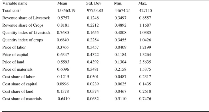
Table 2.1: Variable Summary Statistics 1948-2004………...………51
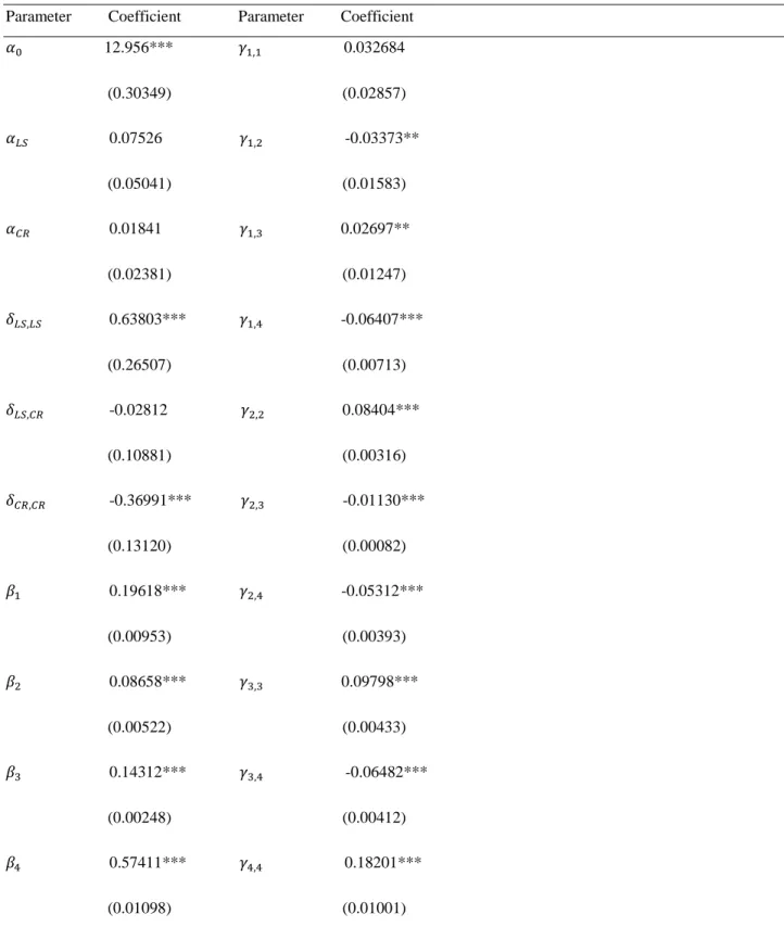
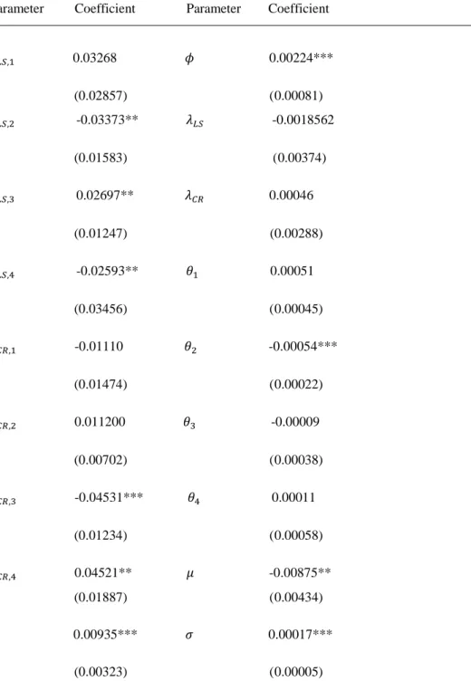
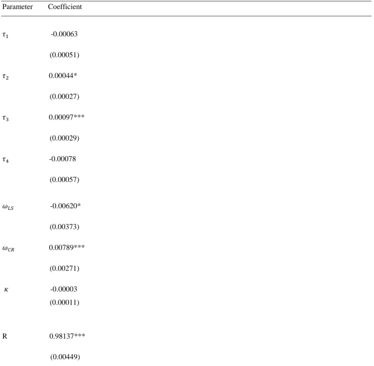
Table 2.2: Parameter estimates of the Translog Cost function for US Agricultural Production ……….52
Table 2.3: Output Bias………...………….55
Table 2.4: 90% Confidence Intervals for Output Bias ………..……56
Table 2.5: Input Bias ………..57
Table 2.6: 90% Confidence Intervals for Input Bias ………...58
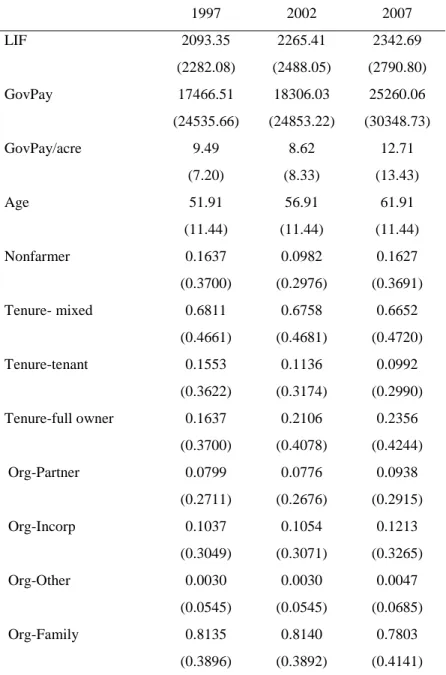
Table 3.1: Descriptive Statistics for Surviving Corn-Soy Producers- Mean (Standard Deviation) 1997-2007………....59
Table 3.2: Descriptive Statistics for Surviving Wheat Producers- Mean (Standard Deviation) 1997-2007………60
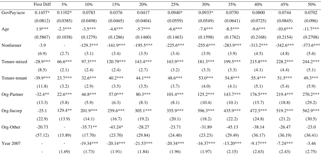
Table 3.3: Panel Data Estimation Results (𝛽(𝜏)), for Farm Operators Classified as Producing Corn and Soy as the Major Crop. The Dependent Variable is Land in Farm…61 Table 3.4: Panel Data Estimation Results (𝛽(𝜏)), for Farm Operators Classified as Producing Wheat as the Major Crop. The Dependent Variable is Land in Farm…………63
Table 3.5: 𝜒2 Statistics for Pairwise Hypothesis Testing on Statistically Significant Marginal Effect Estimates 𝛽(𝜏), for Farm Operators Classified as Producing Corn and Soybeans as the Major Crop ………..65
Page Table 3.6: 𝜒2 Statistics for Pairwise Hypothesis Testing on Statistically Significant Marginal Effect Estimates 𝛽(𝜏), for Farm Operators Classified as Producing Wheat as the Major Crop ……….…….66 Table 4.1: Proportion of Rejection of the Null (t=2)………..……67 Table 4.2 : Proportion of Rejection of the Null (t=7)……….……….68
LIST OF FIGURES
Figure Page Figure 2.1: Output bias due to technical change……….10 Figure 2.2: Input bias due to technical change ………...12 Figure 3.1: Marginal effect of government payments per acre on farm size for operators classified as producing corn and soybeans as major crop………...69 Figure 3.2: Marginal effect of government payments per acre on farm size for operators classified as producing wheat as major crop………...70 Figure 4.1: Power and Size of the MD Framework of Hypothesis Testing (t=2)……..…71 Figure 4.2: Power and Size of the MD Framework of Hypothesis Testing (t=7)……….…72
ABSTRACT
Haque, Samiul. Ph.D., Purdue University, December 2014. US Commodity Support Payments: On Allocation of Resources and Fairness, Post 1996. Major Professor: Kenneth Foster
This dissertation investigates the effect of US commodity support payment on agricultural producer decisions during the “decoupled” regime. Particular attention is paid to the national optimal output mix, input proportions, and farm level changes in scale operations. While “decoupled” payments were instated to comply with WTO guidelines, where tax payer dollars cannot be spent to alter agricultural outputs and /or on farm input decisions, evidence suggests that such payments are far from being decoupled. At the national level, this dissertation finds evidence for mild labor input using and capital input economizing behavior. Substantial land input economizing behavior and moderate material input using behavior due to scale effects of crop production is also observed. However, such a policy does not appear to alter the optimal output mix. The finding that government payments alter the scale of national crop production is further validated while looking at the farm level changes in scale of operation. Farm level data was analyzed using quantile regressions, where the effect of payments on the entire distribution of conditional farm size was quantified. The findings suggest that government payments do increase farm size at
some parts of the conditional distribution and not others, and these effects are bigger for larger farms. This dissertation provides empirical evidence that commodity support programs provide advantage to large farming operations in terms of increasing scale of operation. Perhaps as heterogeneous farmers enlarge or diminish their share of agricultural production, the marketplace systematically selects those with similar management strategies or technological capacities in each case, thus shifting the national production technology.
CHAPTER 1: INTRODUCTION
1.1 Introduction
Farm commodity programs were initially instated during the 1930s Depression when commodity prices were low due to weak consumer demand. Policy makers legislated price support and supply control programs in order to stabilize income of farmers (25% of the US population lived on farms at that time), most of whom were small in scale and diversified, and to ensure abundant supply of food and fiber (CRS 2008). Since the inception of commodity programs, the face of US agriculture has changed substantially with less than 2% of the US population now living on farms and agricultural production has now shifted to larger farm operations. While commodity programs of the 1930s were intended to be temporary, they have survived to this date with numerous modifications. The persistence of commodity programs can no doubt be attributed to a strong agricultural lobby, but one cannot simply ignore the presence of some tangible public support.
This dissertation focuses on the “decoupled” era, starting from the 1996 FAIR Act, where commodity support payments were divorced from market outcomes. The transition from traditional price support and supply control programs to one where payments were tied to historical acreage and yields of program crops was prompted by the impetus to comply with WTO guidelines. Such guidelines required member states to adopt a policy where taxpayer dollars cannot be used to influence production levels and on farm decisions. However, since their inception, there has been significant misgivings both within the academic community and policy circles about the “decoupled” nature of these payments and fairness of disbursements and subsequent economic outcomes.
There are many channels by which decoupled payments might affect production and / or on farm decisions (for reviews, see OECD, 2005 and Bhaskar and Beghin, 2009). While it is not the aim of this dissertation to dissect all the various channels, it should be noted that each of the different research concentrates in some way or another on the potential of decoupled payments to alter agricultural producer behavior. The objective of this dissertation is to inform the misgivings regarding such farm programs in two ways: 1) by introducing a neglected aspect of lump sum transfers in altering the underlying production technology of national US agriculture. In particular, the role of decoupled payments in altering the national output mix (output bias) and relative proportions of input use (input bias) is investigated 2) by addressing the questions about fairness- where higher payment levels accrue to large farm operations simply by design of the program. As such, it has been argued that decoupled payments provide unfair advantage to large farming operations as compared to their smaller counterparts. There is a third contribution of this dissertation, where the finite samples properties of the Minimum Distance estimator framework of hypothesis testing for quantile regression is investigated using Monte Carlo simulations. This contribution should be viewed as complementary to the second objective rather than a standalone goal.
1.2 Overview of the Essays Included in this Dissertation
In this dissertation, the units of observation range from national time series data (chapter 2), individual farm level data (chapter 3), and simulated dataset (chapter 4). While the dissertation is organized to allow each chapter to stand alone as an independent essay, some general conclusions will be drawn in the end (chapter 5).
The first dissertation essay focuses in the econometric estimation of output and input bias of US Direct Payments. The study is conducted on US national agricultural productivity time series data 1948-2011. The empirical framework allows Direct Payments to alter the input and output expansion path. A system of equations consisting of a translog cost function, along with relevant input cost share and output revenue share of cost is
estimated with 3 stage iterative seemingly unrelated regression. The results suggest that such payment programs are mildly labor and capital input economizing, strongly land input economizing, and moderately material input using. Such effects has been largely ignored in the past literature and should provide important considerations in future policy formulation.
The second dissertation essay focuses on econometrically investigates the differential impact of commodity support payments on farm size of US corn-soy and wheat producers. The study was conducted on farm level panel data obtained from US Census of Agriculture (1997, 2002, and 2007). Unlike previous work which focuses on the impacts on the conditional mean, the current approach, using recent advancements in correlated random effects quantile regression model, quantifies the impact of government payments at different locations along the entire conditional distribution of farm size. The results show that government payments increase farm size at some parts of the farm size distribution and not others, and these effects are larger for bigger farms. Both corn-soy and wheat producers at the 85th percentile of the conditional farm size distribution are almost four times more responsive to a dollar increase in commodity payments per acre than those at the 25th percentile. This paper provides empirical evidence that commodity support programs provide unfair advantage to large farming operations.
The third essay investigates the finite sample properties of the Minimum Distance (MD) estimator framework of testing equality of slopes for quantile regressions. This study complements the second dissertation essay where the same hypothesis testing framework is used for statistical inference. Past studies have established that the test statistic has a limiting chi-squared distribution with appropriate degrees of freedom. With applications of quantile regressions on panel data gaining popularity amongst applied econometricians in recent years, it becomes important to investigate the power and size of the MD test for finite sample. Results suggest that the test has under sized and low power in small samples. However, with larger samples, while the power property improves, the test still remains under sized. Given the second dissertation essay utilizes very large sample size, the inferences drawn MD test should not cause concern.
1.3 Reference
Monke, J. 2008. Farm Commodity Programs in the 2008 Farm Bill. Order Code
RL34594, Washington, DC: U.S. Congressional Research Service
Organization for Economic Cooperation and Development (OEDC). 2005. A Review of Empirical Studies of the Acreage and Production Response to US Production Flexibility Contract Payments under the FAIR Act and Related Payments under Supplementary Legislation. Directorate for Food, Agriculture and Fishers Committee for Agriculture.
Bhaskar, A. and Beghin, J.C. 2009. “How Coupled are Decoupled Farm Payments? A Review of the Evidence.” Journal of Agricultural and Resource Economics, 34(1):130-153
CHAPTER 2: ON SOME UNINTENDED CONSEQUENCES OF DIRECT PAYMENTS: A NATIONAL PERSPECTIVE
2.1 Introduction
Direct payments operate as a lump-sum transfer to farm operators with receipts determined solely by historical participation in commodity support programs. These payments were instituted in 2002 to extend production flexibility contracts (PFCs) of the 1996 Farm Bill which overhauled U.S. farm programs to better comply with international trade commitments. As these payments do not depend on market conditions, they are assumed not to affect production levels or on-farm input decisions, and thus qualify as “green box” subsidies, i.e. those subsidies which are least trade distorting in the GATT/WTO lexicon. However, the academic literature has advanced various theoretical models and conducted empirical studies that suggest direct payments do alter production level (albeit minimally) and on-farm input decisions.
Among the extant literature, none thus far has explicitly examined the role of direct payments in altering relative proportion of input use (input bias) and output mix (output bias) at the national level. The objective of this study is to fill the void by econometrically estimating these effects. Analysis of these effects at the national level is crucial to the debate over direct payments since it is at this level that trade distortion will be measured. Literature suggesting that decoupled payments alter output, albeit minimally, and on-farm input use at the farm level, provides the impetus to potentially observe bias in relative input use and or output mix at the national level. Recognizing and estimating such possible impacts would provide important considerations for the development of future agricultural policies.
Hennessy (1998) modeled risk averse producer behavior and showed that the higher average income (wealth effect) and income stabilization (insurance effect) due to direct payments will lead to increased input usage and expected output. Using Kansas farm data, Serra, Goodwin, and Featherstone (2011) found evidence of decreasing absolute risk aversion and increasing relative risk aversion preferences, but found miniscule effect of direct payments on agricultural output. As for acreage response, Goodwin and Mishra (2006) found negligible impact of direct payments. Payments may preserve inefficient producers, but they are not likely to have a marked output impact (Chau and de Gorter, 2005). Also farmers in the crop sector may use direct payments to continue or expand economically non-viable production (Hennessey and Thorne, 2005).
While investigating the effect of direct payments on labor input, El-Osta, Mishra, and Ahearn (2004) found that government payments increase on-farm hours worked by farm operators but the impact was quantitatively very small. This result is at odds with the standard household model theory- lump sum transfers unambiguously should have no effect on on-farm labor. Key and Roberts (2009) reconcile this issue by developing a theoretical model where, with decreasing marginal utility to income, decoupled payments may reduce off-farm work and increase on-farm work. Key and Roberts (2009), reverberating the notions of Hennessey and Thorne (2005), finds compelling evidence for substantial non-pecuniary benefits to farming. On-farm labor may also increase if government payments work to prevent exit of non-profitable farms as suggested by Chau and de Gorter (2005).
Under incomplete credit markets, the effects of these lump sum transfers can be significant. A credit constrained farmer may use direct payments for more on-farm investment and production (Collender and Morehart, 2004). This is assuming that the return to investment is higher than the interest rate available in the credit market, while a loan could not be obtained. Goodwin and Mishra (2006) found that the interaction of producer flexibility contract with a producer’s debt to asset ratio, has a small negative influence on the number of acres idled. Kropp and Whitaker (2011) concludes that because of capital cost reduction due to direct payments, some farms may increase input use or
operate on land that would be otherwise be unprofitable. Roe, Somwaru, and Diao (2008) suggests that direct payments improve access to credit for producers both by directly increasing their wealth, and through a higher land price that increases the collateral.
Given decoupled payments are tied to land holdings, the landlord then is likely to appeal to the inelastic supply of land and try to capture most of the subsidy through higher land rent. In turn, this increases land values; Roberts, Kirwan, and Hopkins (2003), and Goodwin, Mishra, and Ortalo-Magne (2003) find credible evidence of capitalization of direct payments in land values. Higher land prices translate into higher input costs over time for producers and decrease the return to investment. If, in fact, landowners capture most of the direct payment dollars, tenants might either substitute away from land in favor of other inputs and/or decrease crop production intensity. Additionally, the tenants might decide to focus more on livestock production, assuming that it requires lower land input. It is important to recognize, however, that landlords might not always be able to capture a greater share of the direct payment dollar. Kirwan (2009) found a 25/75 landlord-tenant split of the marginal subsidy dollar. The reason cited is less than perfectly competitive land markets. Farm consolidation and growth has resulted in fewer and larger scale tenants who are likely to exercise greater market power in the land rental market. Thus landlords who forgo the use value of land without a tenant might be willing to compromise and share the subsidy to attract tenants. We would add that observable heterogeneity in farm management and land stewardship among tenants in local markets further exacerbates the lack of competition in rental markets.
Furthermore, there is evidence of positive association between government payments and farm business survival (Key and Roberts, 2006), likelihood of survival and a small yet positive impact on the size of surviving farms (Key and Roberts, 2007), and subsequent growth in farmland concentration (Roberts and Keys, 2008). However, the implication for aggregate market outcome is less clear. For, example, O’Donoghue and Whitaker (2010) constructed a pseudo panel from the ARMS data and utilized the exogenous change in the 2002 Farm bill that allowed oil seeds to be included. They found that direct payments increase individual acreage by 9-16%. While Weber and Key (2012)
make use of same policy variation on the NASS data at the zip code level, and found little effect on aggregate production.
As heterogeneous farmers enlarge or diminish their share of agricultural production due to direct payments, it is credible that the market generated composition of the agricultural sector will shift to a higher proportion of managerially innovative farms. As such, it gives rise to the possibility of altering the national production technology and observing changes in agricultural input intensities and output mix. Understanding these net impacts from direct payments thus calls for a study that employs national data. We follow in the tradition of other studies on US agricultural technology (e.g. Binswanger 1974; Ray 1982) and adopt a cost minimization approach where the mechanism through which direct payments affect input and output bias is specifically identified.
2.2 Modeling Framework
We assume a cost minimizing representative producer to proxy for the aggregate technology with the following objective function:
𝐶(𝑤, 𝑞, 𝑡) ≡ 𝑚𝑖𝑛𝑥 𝑤′𝑥| 𝑥 ∈ 𝐹(𝑥, 𝑞, 𝑡) (2.1)
where C is cost, w is a vector of prices corresponding to inputs x, q is a vector of outputs,
t is an exogenous variable that is a proxy for underlying technology, and F(x,q,t) is a production possibilities set. Estimation of the cost model proceeds by deriving the output compensated demand function, and inverse supply function (under perfect competition) via Shephard’s lemma and estimating them as a system. That is,
𝑥(𝑤, 𝐸𝑞, 𝑡) =𝜕𝐶(𝑤,𝐸𝑞,𝑡)𝜕𝑤 (2.2)
and
where equation (2.3) represents output price (p) equal to marginal cost in the output markets. In the production economics literature, it has become common practice to proxy the technology index, t, with a time trend. The time trend is likely correlated with private and public research and development, research and extension, changes in relative input and output prices, etc. In order to examine our hypothesis that direct payments alter the underlying agricultural production technology, we propose to allow technological change to also be induced by farm policy payments. We accomplish this by including a direct payment policy variable in the model in addition to the time trend. Direct payment outlays follow a more varied and less strongly trended path over time and this reduces the chance of mistakenly capturing only a host of trended factors in the measurement of technical change.
This analysis uses a standard translog cost function. The translog functional form has been successfully applied to aggregate data in a variety of contexts, and represents a flexible second order approximation to the true cost function (see Jorgensen, Christensen, and Lau 1973). We specify the cost function as a function of four input prices, and two outputs: 𝑙𝑛𝐶 = 𝛼0+ ∑2 𝛼𝑖𝑙𝑛𝑞𝑖+ 𝑖=1 1⁄ ∑2 𝑖=12 ∑𝑗=12 𝛿𝑖,𝑗𝑙𝑛𝑞𝑖𝑙𝑛𝑞𝑗+ ∑4𝑟=1𝛽𝑟𝑙𝑛𝑤𝑟 + 1 2⁄ ∑ ∑4 𝛾𝑟,𝑠𝑙𝑛𝑤𝑟𝑙𝑛𝑤𝑠 𝑠=1 4 𝑟=1 + ∑𝑖=12 ∑4𝑟=1𝜌𝑖,𝑟𝑙𝑛𝑞𝑖𝑙𝑛𝑤𝑟+𝜑𝑙𝑛𝑧 + 1 2⁄ ϕ(𝑙𝑛𝑧)2+ ∑2 𝜆𝑖𝑙𝑛𝑧𝑙𝑛𝑞𝑖+ 𝑖=1 ∑4𝑟=1𝜃𝑟𝑙𝑛𝑧𝑙𝑛𝑤𝑟+ 𝜇𝑡 + 1 2⁄ 𝜎𝑡2+ ∑𝑟=14 𝜏𝑟 tln𝑤𝑟+ ∑2𝑖=1𝜔𝑖𝑡𝑙𝑛𝑞𝑖 + 𝜅𝑡𝑙𝑛𝑧 (2.4)
where ln is the natural logarithm; z denotes the level of government farm payments; 𝑖( j) index quantities of livestock and crop outputs; r(s) index prices of labor, capital, land, and material inputs. By assuming that farmers are price takers in input and output markets, we can use Shepherd’s Lemma to derive the factor cost and output specific revenue (relative to total costs) equations.
We follow past studies (e.g Kuroda 1988; Kuroda and Lee 2003) to adopt a measure of change in output mix (output bias) due to direct payments from Capalbo and Antle (1988). For the two-output cost function, this measure of output bias can be constructed in terms of movement of the expansion path in the output space and defined as follows:
𝐵𝑖,𝑗𝑄 ≡ 𝜕𝑙𝑛( 𝜕𝐶 𝜕𝑞𝑖 𝜕𝐶 𝜕𝑞𝑗 ⁄ ) 𝜕𝑙𝑛𝑧 = 𝜕𝑙𝑛(𝜕𝐶 𝜕𝑞𝑖) 𝜕𝑙𝑛𝑧 − 𝜕𝑙𝑛(𝜕𝐶 𝜕𝑞𝑗) 𝜕𝑙𝑛𝑧 = 𝜕𝑙𝑛𝑀𝐶𝑖 𝜕𝑙𝑛𝑧 − 𝜕𝑙𝑛𝑀𝐶𝑗 𝜕𝑙𝑛𝑧 (2.5),
where 𝐵𝑖,𝑗𝑄 measures the rotation of the production possibility frontier at a point. The term(s) 𝜕𝑙𝑛𝑀𝐶𝑖(𝑗)
𝜕𝑙𝑛𝑧 can be interpreted as the government payment elasticity of marginal cost
for output i(j). Technical change in the output space is said to be biased towards output i, j, or Hicks neutral if 𝐵𝑖,𝑗𝑄 < 0, 𝐵𝑖,𝑗𝑄 > 0, or 𝐵𝑖,𝑗𝑄 = 0. We can write an expression for 𝐵𝑖,𝑗𝑄 in terms of model parameters as 𝜀𝜆𝑖
𝐶𝑞𝑖− 𝜆𝑗 𝜀𝐶𝑞𝑗, where 𝜀𝐶𝑞𝑖 = 𝜕𝑙𝑛𝐶 𝜕𝑙𝑛𝑞𝑖 = 𝛼𝑖 + ∑ 𝛿𝑖,𝑗𝑙𝑛𝑞𝑗 + 2 𝑗=1
∑4𝑟=1𝜌𝑖,𝑟𝑙𝑛𝑤𝑟+ 𝜆𝑖𝑙𝑛𝑧+ 𝜔𝑖𝑡 (see Appendix A for details). We illustrate output bias in
Figure 2.1 below:
Figure 2.1: Output Bias due to Technical Change
T2 T1 E2 T2 E1 e(z2,t) e(z1,t) P1 P1 P2 T1 qi qj
Let e(z1,t) be the initial expansion path in the output space, i.e. the set points reflecting
least cost method of producing different levels of output, when output prices remain constant. The firm produces at point E1, where the isoquant T1 T1 is tangent to the
isorevenue line P1. Technological change due to direct payment causes the new expansion
path to be say e(z2,t). The new production possibility frontier is T2 T2 which passes through
the point E1. 𝐵𝑖,𝑗𝑄 measures the a hypothetical rotation of the isorevenue line P1 tangent to
T1 T1 at E1,to P2 tangent to T2 T2.
A second goal of this study is to estimate the degree to which government payment led technical change induces bias in relative input use as well as scale effects in production. In developing these measures, we follow the approach outlined in Capalbo and Antle (1988) which extends the multi-output form of Binswanger’s (1974, 1978) dual measure of input bias for a non-homothetic cost function. Capalbo and Antle (1988) define bias over the general index of technology, t; in our application bias is measured over the policy variable z. Thus, the measure of input bias,𝑀𝐵𝑟𝑐, is defined as:
𝑀𝐵𝑟𝑐 = 𝜕𝑙𝑛𝑆𝑟
𝜕𝑙𝑛𝑧
⁄ = 𝜃𝑟
𝑆𝑟
⁄ (2.6), where 𝑆𝑟 is the share of input r in total cost. 𝑀𝐵𝑟𝑐 measures the relative change in factor proportions brought about by direct payments. A positive (negative) value of 𝑀𝐵𝑟𝑐 indicates that direct payment is rth factor using (saving) relative to all other factors of
production. 𝑀𝐵𝑟𝑐=0 implies direct payment is neutral, i.e. factor proportions are invariant
to payment levels. If the technology is non-homothetic, i.e. if the firm’s expansion path in the input space is non-linear, the input bias measure in (2.6) has to be adjusted for the scale effect, due to movement along the expansion, to obtain the pure bias effect. The pure bias of input due to shift in the expansion path for non-homothetic technology is (Antle and Capalbo (1988)):
𝑀𝐵𝑟𝑐𝑒 = 𝑀𝐵
𝑟𝑐 − [∑ (𝜕𝑙𝑛𝑠𝑖 𝑟/𝜕𝑙𝑛𝑞𝑖)(𝜕𝑙𝑛𝐶/𝜕𝑙𝑛𝑞𝑖)−1] 𝜕𝑙𝑛𝐶/𝜕𝑙𝑛𝑧 (2.7).
Alternatively, equation (2.7) can be denoted in terms of the model parameters, with
(𝜑 + ϕ𝑙𝑛𝑧 + ∑2𝑖=1𝜆𝑖𝑙𝑛𝑞𝑖+ ∑4𝑟=1𝜃𝑟𝑙𝑛𝑤𝑟+𝜅𝑡). Taken together, we can rewrite pure bias of input (2.7) as: 𝑀𝐵𝑟𝑐𝑒 = 𝜃𝑆𝑟 𝑟− 𝜋𝜌1𝑟 𝑆𝑟𝜀𝑐𝑞1 − 𝜋𝜌2𝑟 𝑆𝑟𝜀𝑐𝑞2 (2.8). The first term on the right hand side of (2.8) is the same as (2.6), the second term measures the scale effect due to livestock production, and the third term measures the scale effect due to crop production. Note that these measures bias and scale effects are interpreted as elasticities. To facilitate exposition let us consider Figure 2.2 below:
Figure 2.2: Input Bias due to Technical Change
Let the initial expansion path in the input space be e(z1,t), i.e the set of points associated
with the least cost method of producing different levels of output, given constant input prices. The firm produces at point A. After technical change we have a new expansion path e(z2,t) and the firm produces at point C. Technological advancement has reduced the
cost of producing output Q1 as shown by the movement from A to C. This movement has
two components. One is the scale effect, from A to B, change in factor share along a given expansion path due to change in output levels. The other is the pure bias effect, from B to
Xr Xs e(z1,t) e(z2,t) Q1 (z1t) Q1 (z2t) A B C
C, representing the shift in the isoquant line along the same isocost line, and the consequent change in factor share.
2.3 Data
Data describing input prices and output quantities were obtained from national agricultural productivity statistics published the U.S. Department of Agriculture (USDA 2012a) for 1948-2011. Information describing farm program payments are available from farm income and wealth statistics published by U.S Department of Agriculture (USDA 2012b). In this analysis PFC payments from 1996-2002 and direct payments (DP) from 2002-2011 are included. The agricultural productivity dataset contains price and quantity indices of agricultural outputs and inputs that can be used in the estimation of the cost function. Farm data was aggregated into two outputs: livestock and crops, and four inputs: labor, capital, land, and material goods. Labor inputs includes both hired and self-employed labor. The capital input consists of a range of inputs such as durable equipment, service buildings, and inventories. Material inputs include energy, fertilizer and lime, pesticides, purchased services, and other intermediate inputs. Aggregate measures of quantities and prices were calculated using the Fisher Index, with 2005 as the base year (also point of approximation). The summary statistics is provided in table 2.1.
A couple aspects of this dataset makes it particularly suited for our study. First, output prices correspond to the value of output to the producer, i.e., subsidies are added and indirect taxes are subtracted from market values. The price received by farmers include allowance for net Commodity Credit Corporation loans and purchases by the government valued at the average loan rate. However, direct commodity payments are not reflected in to price data. This implies, while our variable for direct payments in a series of “zeroes” prior to 1996, all “coupled” subsidies are directly incorporated into output prices (p) and enters our model through the inverse supply function (2.3). This attribute of the dataset assures us that we are in fact observing the impact of direct payments on the production technology. Second, land area diverted from production under federal commodity
programs and Conservation Reserves are excluded from the stock of land. This ensures that we are not incorporating land input that is not directly used in agricultural production. An excellent and detailed description of the methods used to construct the indices is documented in Ball, Bureau, Nehring, and Somwaru (1997) and Ball, Wang, and Nehring (2012).
2.4 Estimation Strategy
Estimation was performed on a system of equations derived from a standard translog cost function specification:
𝑙𝑛𝐶𝑡 = 𝛼0+ ∑2 𝛼𝑖𝑙𝑛𝑞𝑖,𝑡+
𝑖=1 1⁄ ∑2 𝑖=12 ∑𝑗=12 𝛿𝑖,𝑗𝑙𝑛𝑞𝑖,𝑡𝑙𝑛𝑞𝑗,𝑡+ ∑4𝑟=1𝛽𝑟𝑙𝑛𝑤𝑟,𝑡 +
1 2⁄ ∑𝑟=14 ∑4𝑠=1𝛾𝑟,𝑠𝑙𝑛𝑤𝑟,𝑡𝑙𝑛𝑤𝑠,𝑡+ ∑𝑖=12 ∑4𝑟=1𝜌𝑖,𝑟𝑙𝑛𝑞𝑖,𝑡𝑙𝑛𝑤𝑟,𝑡+𝜑𝑙𝑛𝑧𝑡+ 1 2⁄ ϕ(𝑙𝑛𝑧𝑡)2 +
∑𝑖=12 𝜆𝑖𝑙𝑛𝑧𝑡𝑙𝑛𝑞𝑖,𝑡+∑4𝑟=1𝜃𝑟𝑙𝑛𝑧𝑡𝑙𝑛𝑤𝑟,𝑡+ 𝜇𝑡 + 1 2⁄ 𝜎𝑡2 + ∑4𝑟=1𝜏𝑟 tln𝑤𝑟,𝑡+
∑2𝑖=1𝜔𝑖𝑡𝑙𝑛𝑞𝑖,𝑡+ 𝜅𝑡𝑙𝑛𝑧𝑡+ 𝜖𝑡 (2.9)
The associated cost and revenue share equations can respectively be written as:
𝑆𝑟 = 𝛽𝑟+ ∑4𝑠=1𝛾𝑟,𝑠𝑙𝑛𝑤𝑠,𝑡+∑2𝑖=1𝜌𝑖,𝑟𝑙𝑛𝑞𝑖,𝑡+𝜃𝑟𝑙𝑛𝑧𝑡+ 𝜏𝑟𝑡 + 𝜂𝑡 (2.10)
and
𝑅𝑖 = 𝛼𝑖 + ∑4 𝜌𝑖,𝑟𝑙𝑛𝑤𝑟,𝑡+
𝑟=1 ∑2𝑗=1𝛿𝑖,𝑗𝑙𝑛𝑞𝑗,𝑡+𝜆𝑖𝑙𝑛𝑧𝑡+ 𝜔𝑡𝑡 + 𝑜𝑡 (2.11),
where 𝑅𝑟 is the revenue share of output r in total cost. We impose the following restriction on the cost function to maintain homogeneity of degree one in factor prices: ∑4𝑟=1𝛽𝑟 = 1,
∑4 𝛾𝑟,𝑠
𝑠=1 = 0, ∑4𝑟=1𝜌𝑖,𝑟= 0, ∑𝑟=14 𝜃𝑟 = 0, and ∑4𝑟=1𝜏𝑟 = 0. Furthermore, symmetry
implies: 𝛿𝑖,𝑗= 𝛿𝑗,𝑖 and 𝛾𝑖,𝑗 = 𝛾𝑗,𝑖.
Initially parameters were estimated using the system of equations consisting of the cost function (2.9), three of the four cost share equations (2.10), and the two output specific revenue over cost equations (2.11) using an iterative SUR. Preliminary results suggested serial correlation of the residuals was a problem, so we used a standard method for estimating a common serial correlation coefficient for each equation (Berndt and Savin 1975). This approach maintains the invariance property of the parameter estimates to the
share equation which is dropped from the estimation procedure. Furthermore, our cost function specification treats output quantities as predetermined. However, econometrically output quantities are endogenous to input decisions and total costs. To address this endogeneity, we estimated a first stage OLS of output quantities on a set of variables that are assumed to effect output, namely: input quantities, government payments, and time trend. Since our cost function is non-linear both in terms of variables and parameters we specified a second order polynomial (translog in particular) for the first stage regression following Kelejian’s (1971) and Aemiya’s (1974) suggestion. The predicted values from the first stage were used to estimate the system of cost function. The system of equations was estimated using 3-stage non-linear iterative SUR procedure. Subsequently both input and output bias elasticities were computed from the parameter estimates and data. It is important to know the precision of these elasticity estimates. Therefore we conducted a parametric bootstrap approach to generate an empirical distribution of parameters by randomly sampling from the residuals of the 3-stage non-linear iterative SUR estimation (Dorfman, Kling, and Sexton, 1990). To preserve the cross-correlation structure of the system, we randomly drew with replacement contemporaneous residuals. This was conducted two thousand times to create empirical distribution of parameters. These distributions of parameters were then used to construct confidence intervals for the elasticities.
2.5 Results
At the point of approximation (year 2005), our fitted model i) is non-decreasing in input prices and output quantities ii) has negative own price elasticites of demand for labor, capital, land, and material. Parameter estimates for the model and their standard errors are reported in Table 2.2. For the estimated cost function, five of the eight interactions of input prices with output quantities (ρ) are statistically significant. This implies that the production technology is non-homothetic. Thus requiring adjustment for the scale effects of production in computing input bias (2.7). Note that the actual magnitude of the input
and output bias elasticities is non-linear combination of random variables, and cannot be inferred from the parameter estimates. Furthermore, the precision of these elasticities has to be assed via bootstrapping.
2.5.1 Output Bias
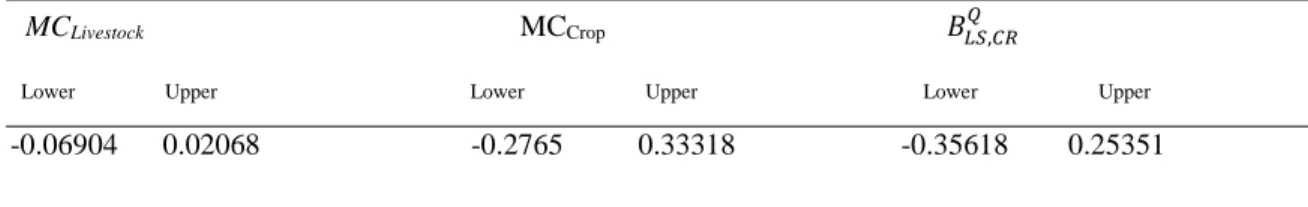
Estimates for direct payment elasticity of marginal cost and Hicksian output bias are presented in Table 2.3 and the associated confidence intervals are reported in Table 2.4. It should be noted that these estimated elasticities are statistically insignificant. Direct payment elasticities of marginal cost for livestock and crop production are -0.0247 and 0.02494 respectively. They imply, ceteris paribus, a 10% increase in direct payments at the point of approximation may decrease the marginal cost for livestock production (by 0.247%) and increase that of crop production (by 0.2494%). Not surprisingly, our estimate for Hicksian output bias (-0.04964) suggests small livestock favoring technological change at the national level due to direct payments. Ceteris paribus, our point estimate of Hicksian output bias suggests that increasing direct payments by 10% may decrease the marginal cost of livestock output relative to that of crops by approximately 0.496%. Such a change in the relative marginal cost of livestock to crops may represent a significant impact in the national markets for commodities and production inputs.
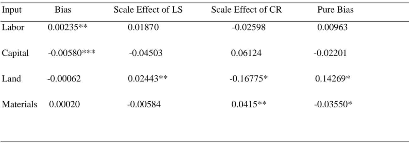
2.5.2 Input Bias
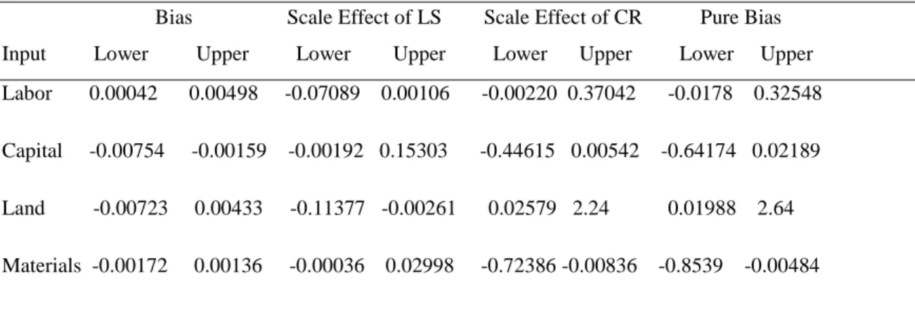
Table 2.5 reports the point estimates for the input bias, scale effects, and pure bias effects (input bias minus the scale effects of production) of factor inputs, and the associated confidence intervals are reported in Table 2.6. Our estimates of input bias (as measured by (2.6)) suggests small changes in relative factor use did occur in the agricultural input sector due to direct payments. This overall measure of input bias suggests that direct payment induced technical change in favor of labor and materials inputs, and against capital and land inputs. For labor input, our bias estimate of 0.00235 significant at the 5% level implies,
ceteris paribus, a 10% increase in direct payments at the point of approximation may increase the cost share of labor input relative to all other factors of production be 0.0235%. For capital inputs, our bias estimate of -0.00580 significant at the 1% level implies, ceteris paribus, a 10% increase in direct payments at the point of approximation may decrease the relative cost share of capital input by 0.058%. However, using this measure it is not clear whether this bias is due to the direct impact of payments on relative factor use or is the artifact of an indirect impact of payments on the scale of farming operations in the presence of non-homothetic technology.
The scale effects of production reveal distinct factor intensities for livestock versus crop production. Our point estimates suggest that direct payments induced scale effects in livestock production is labor and land input using, and capital and material inputs saving. For crop production, direct payment induced scale effect is labor and land input saving, and capital and material inputs using. Our estimate of direct payment induced scale effect of land in livestock production (0.02433) significant at the 5% level suggests, ceteris paribus, a 10% increase in direct payments at the point of approximation may increase the relative cost share of land input by 0.2433%. While the scale effect of land in crop production (-0.16775) significant at the 10% level suggests, ceteris paribus, a 10% increase in direct payments at the point of approximation may decrease the relative cost share of land input by 1.6775%. And the scale effect of material inputs (0.0415) in crop production significant at the 5% level implies, ceteris paribus, a 10% increase in direct payments may increase the relative cost share of material inputs by 0.415%.
Finally our estimates of pure bias effects (as measured by (7)) suggests bias in favor of labor and land input, and against capital and material inputs. This measure captures the change in input factor cost share due to shift in the input expansion path due to direct payments. Our estimate for pure bias effect of land (0.14269) significant at the 10% level suggests, ceteris paribus, a 10% increase in direct payments at the point of approximation may increase the relative cost share of land input by 1.4269%. Our estimate for pure bias effect of material input (-0.03550) significant at the 10% level suggests, ceteris paribus, a 10% increase in direct payments at the point of approximation may decrease the relative
cost share of material input by 0.355%. Note that much of the pure input bias is driven by quantitatively large scale effect of production induced by direct payments. Our findings suggests that direct payments induced changes in relative input use for the national US agriculture are driven by substantial scale effects and not inherent bias effects.
2.6 Conclusions
This article examines the extent to which direct payments to agricultural producers have induced changes in output mix and input intensity for national U.S. agriculture. We found that direct payments have a statistically insignificant effect of decreasing the marginal cost of livestock production and increasing the marginal cost of crop production. But what may explain this qualitative result? In the US, the livestock sector is the recipient of zero direct payments. Perhaps what our result for the livestock sector implies- in the absence of lump sum transfers from the government, the least efficient livestock producers exit. Thus lowering the national marginal cost for the sector. In contrast, the crop sector, which receives all the Direct Payments may preserve inefficient producers and thus increasing the national marginal cost. Such notions are also consistent with generalizations of the analytical findings of Chau and de Gorter (2005). Furthermore, farmers in the crop sector may use direct payments to continue or expand economically non-viable production (Hennessey and Thorne, 2005).
Our results does show that direct payments do have some unintended statistically significant effect of altering input intensities for the national US agriculture. It is worth reiterating that these are all relative measures. For example, it is possible that the absolute amount of a particular input has increased, but its cost share relative to all other factors of production has declined. Overall input bias suggests that direct payments are labor using and capital economizing. While technological innovation has reduced the cost of capital inputs for US agriculture in general and contributed towards substitution of labor for capital, it seems that direct payments has acted to mildly mitigate this trend. One may possibly argue that direct payments are contributing to the sustainability of rural America
by keeping labor in farms. However, to what extent such an outcome is aligned with broader policy objectives is a matter of open discourse.
Our study finds substantial scale effect generated by direct payments to farmers, particularly in the market of land, which is driving the changes in relative inputs use (pure bias). Notice that that scale effects of production is greater than bias effects by order of magnitude (one to three). These scale effects are the combined result of induced scale adjustments and non-homothetic nature of the underlying technology. The scale effect of livestock production is mildly land using and that of crop production is strongly land economizing. Our estimated scale effect of land in crop production (-0.16775), while inelastic, is economically very significant. Given credible evidence of capitalization of direct payments into land values (Roberts, Kirwan, and Hopkins (2003), and Goodwin, Mishra, and Ortalo-Magne (2003)), it makes sense that we observe land economizing behavior in the crop sector. At the national level, one would expect inelastic response of land share of total cost as output changes due to direct payments. Furthermore, considering that inputs of agricultural production are not allocated by outputs, let alone by program and non-program crop, makes our estimated elasticity of scale effect of land in crop production to be considerably large. While political will to cut budgets appears to be growing, policy makers should consider the spillover implications of these decisions, particularly in terms of a land price bubble burst. Land is not only a factor of production in agriculture, but often viewed as an asset against which credit is obtained. If commodity payments tied to agricultural land is discontinued, it is likely to have sector wide ramification rather than just on the recipients.
Given that we have found statistically insignificant impacts of direct payments in altering the marginal cost of both livestock and crop production, what might be driving such substantial scale effects of production? It would seem reasonable to believe that for direct payments to alter the scale of agricultural production, it has to lower the marginal cost of production. This line of reasoning is consistent with notion that agricultural producers are strictly profit maximizing agents. However, given past evidence of non-pecuniary benefits to farming (Key and Roberts (2009) & Hennessey and Thorne (2005)),
it is possible that production decisions are not taken solely based on marginal cost pricing. In addition, it is likely that the wealth effects due to direct payments might have had a role in affecting the relative risk aversion of farmers which resulted in further scale of production.
The scale effect of crop production is also accompanied with moderate material input expansion. Given that direct payments are not tied to material inputs, perhaps our result is indicating that the representative national producer is switching to material input from land input. This outcome might come as a welcoming news to suppliers of energy, fertilizer and line, pesticides, purchased services, and other intermediate inputs, albeit marginally. From a policy perspective, the extent to which existing land is farmed through intensive use of material inputs (fertilizer, lime, energy, etc.) might be associated with some negative externalities such as farm runoff and higher greenhouse gas emissions. While evaluating such impact is beyond the scope of this research, we think that it is a promising avenue for future work.
2.7 References:
Amemiyia, T. 1974. “The non-linear two-stages least squares estimator.” Journal of Econometrics 2(2):105–110
Ball, V.E., Bureau, J.C., Nehring, R., and Somwaru. A. 1997. “Agricultural Productivity Revisited,” American Journal of Agricultural Economics 79: 1045-1063. Ball, V.E., Wang, S.L., and Nehring, R. 2012. Agricultural Productivity in the U.S.:
Findings, Documentation and Method. Economic Research Service, U.S.
Department of Agriculture. Available at
http://www.ers.usda.gov/data- products/agricultural-productivity-in-the-us/findings,-documentation,-and-methods.aspx#.VD3wdGO_6vA Accessed March 2012.
Berndt R. E., and Savin, N. E. 1975. “Estimation and hypothesis testing in singular equations systems with autoregressive disturbances.” Econometrica, 43(5/6): 937-958
Binswanger, H. 1974. “The Measurement of Technical Change Biases with Many Factors of Production.” American Economic Review 64: 964-976.
Binswanger, H. 1978. “Measured Biases of Technological Change: The United States,” in
H. Binswanger and V. Ruttan, eds. Induced Innovation: Technology,
Institutions, and Development, Baltimore, Johns Hopkins University Press. Capalbo, S.M, and Antle, J.M. eds. 1988. Agricultural Productivity: Measurement and
Explanation. Washington, D.C., Resources for the Future, Johns Hopkins University Press, 403
Chau, N. H., and de Gorter, H. 2005 “Disentangling the Consequences of Direct Payment Schemes in Agriculture on Fixed Costs, Exit Decisions, and Output.” American Journal of Agricultural Economics 87(5): 1174-1181.
Christensen, L.R., Jorgenson, D.W, and Lau, L.J. 1973. “Transcendental Logarithmic Production Frontiers.” The Review of Economics and Statistics, 55(1): 28-45 Collender, R.N., and Morehart, M. 2004. Decoupled Payments to Farmers, Capital
Markets, and Supply Effects. Washington, DC: U.S Department of Agriculture, ESCS For. Agr. Econ. Rep. 838, October.
Dorfman, J.H, Kling, C.L, and Sexton, R.J. 1990. “Confidence Intervals for Elasticities and Flexibilities: Reevaluating the Ratio of Normals Case.” .” American Journal of Agricultural Economics 72(4): 1006-1017.
El-Osta, H.S, Mishra, A.K., and Ahearn, M.C. 2004. “Labor Supply by Farm Operator Under “Decoupled” Farm Program Payments.” Review of Economics of the Household 2: 367-385
Goodwin, Barry K., Mishra, Ashok K, and F. Ortal Magne. (2003). “What’s Wrong With Our Models of Agricultural Land Values.” American Journal of Agricultural Economics, 85(3), pp. 744-752
Goodwin, B., and Mishra, A. (2006). “Are ‘Decoupled’ Farm Program Payments Really Decoupled? An Empirical Evaluation.” American Journal of Agricultural Economics 88: 73-89.
Hennessy, D. (1998). “The Production Effects of Agricultural Income Support Policies Under Uncertainty.” American Journal of Agricultural Economics 80(1): 46–57. Hennesy, D.A., and Thorne, F.S. 2005. “How Decoupled are Decoupled Payments? The
Evidence from Ireland.” EuroChoices 4(3): 30-35
Kalejian, H. 1971. “Two-stage least squares and econometric systems linear in parameters and non-linear in endogenous variables.” Journal of American Statistical Association 66:373–374
Key, N., and Robers, M.J. 2009. “Nonpecuniary Benefits to Farming: Implications for Supply Response to Decoupled Payments.” American Journal of Agricultural Economics 91(1): 1-18.
Key, N., and Roberts, M.J. 2006. 2007. “Do Government Payments Influence Farm Size and Survival?” Journal of Agricultural and Resource Economics 32(2):330–48. Key, N., and Roberts, M.J. 2006. “Government Payments and Farm Business Survival.”
Kirwan, B. 2009. “The Incidence of U.S Agricultural Subsidies on Farmland Rental Rates.”
Journal of Political Economy 117(1): 138-164
Kropp, J.D., and Whitaker, J.B. 2011. “The Impact of Decoupled Payments on the Cost of Operating Capital.” Agricultural Finance Review 71(1): 25-40
Kuroda, Y. 1988. "The Output Bias of Technological Change in Postwar Japanese Agriculture." American Journal of Agricultural Economics 70:663-73.
Kuroda, Y., and Lee, Y.S. 2003. “Output and Input Biases Caused by Public Agricultural Research and Extension in Japan, 1957–1997.” Asian Economic Journal. Vol 17 No 2. Pp105-128
Ray, S. 1982. “A Translog Cost Function Analysis of U.S. Agriculture, 1939-1977,”
American Journal of Agricultural Economics 64: 490-498.
O’Donoghue, E.J., and Whitaker, J.B. 2010. “Do Direct Payments Distort Producers’ Decisions? An Examination of the Farm Security and Rural Investment Act of 2002.” Applied Economic Perspectives and Policy. 32(1): 170–193.
Roberts, M.J., Kirwan, B., and Hopkins, J. 2003. “The Incidence of Government Porgram Payment on Agricultural Land Rents: The Challenges of Identification.”
American Journal of Agricultural Economics 85(3): 762-769.
Roberts, M. J., and Key, N. 2008. “Agricultural Payments and Land Concentration: A Semi-Parametric Spatial Regression Analysis.” American Journal of Agricultural Economics 90(3), pp. 627-643.
Roe, T., Somwaru, A., and Diao. X. 2003. “Do Direct Payments Have Intertemporal Effects on US Agriculture?” In C.B. Moss and A. Schmitz, eds. Government Policy and Farmland Markets, pp. 115–39. Ames, IA: Iowa State Press.
Teresa Serra, Barry K. Goodwin, Allen M. Featherstone. (2011). “Risk behavior in the presence of government programs.” Journal of Econometrics, Volume 162, Issue 1, May 2011, Pages 18-24
U.S. Department of Agriculture. 2012a. Agricultural Productivity in the U.S., available at
http://www.ers.usda.gov/data-products/agricultural-productivity-in-the-us.aspx
Accessed March, 2014.
U.S. Department of Agriculture. 2012b. U.S and State-Level Farm Income and Wealth Statistics, available http://www.ers.usda.gov/data-products/farm-income-and-wealth-statistics/#.VD3unmO_6vB Accessed March, 2014.
Weber, J.G. and Key, N. 2012 “How much Do Decoupled Payments Affect Production? An Instrumental Variable Approach with Panel Data.” American Journal of Agricultural Economics4 (1): 52-66.
CHAPTER 3: DIFFERENTIAL IMPACT OF GOVERNMENT PAYMENTS ON FARM SIZE: EVIDENCE FROM QUANTILE ESTIMATION ON PANEL DATA
3.1 Introduction
The US agricultural commodity support program stemming from the 1996 FAIR Act decouples receipt of government payments from market outcome; instead, these payments are based on historical acreage and yield of program crops. Higher payment levels accrue to operators of large farms simply by design of the program; and over time, with production shifting toward operators of large farms (Hoppe, MacDonald, and Korb 2010; MacDonald 2011), these payments have become increasingly concentrated. For example, between 1995 and 2012 the top 10% of the commodity payment recipients were paid 77% of commodity payments (Environmental Working Group (EWG)).
U.S public opinion reveals that taxpayers would rather see their tax dollars go to small family farms than to large farms (Ellison, Lusk, and Briggerman 2010). Furthermore, interest groups and newspaper editorials have expressed concern about the fairness of commodity support programs. Their apprehension- large corporate farms and agribusiness partnerships have a competitive advantage over small farms in terms of availability of capital, scale economies, and overall profitability. Taxpayer dollars to large farm operations are reinvested in capital and land which further increases their competitive advantage (EWG 2000). Some are even suggesting a subsidy induced cycle – as large farms get even bigger, they become eligible for more government payments, and buy up even more small farms (Riedl 2004). Also, high farmland prices price small farmers and newcomers out of the market (Bakst and Katz 2013). Such concerns have been reverberated in calls to reconsider the distribution of farm subsidies (Becker 2002; Grunwald 2007). As such, it becomes important to answer the question: do government payments cause large
farms to grow more than small farms? Are the differences in marginal effect of government payments between large versus small farms substantial and significant?
Unobserved heterogeneity amongst farm operators makes it difficult to isolate causal effects of government payments on farm size. For example, the unobserved productivity of a farm operator is likely to affect farm size; with more productive operators perhaps managing larger operations, despite being a recipient of government outlays. Also, the receipt of government payments is largely based on historical participation in commodity support programs. It is likely that transaction costs affected the decision to participate in commodity programs. The participation is specific to the individual farm operator, as such, one cannot simply ignore the correlation between the farm operator specific effects and government payments.
Unlike past studies that focus on shifts of the conditional mean, this article, using a correlated random effects quantile regression model, identifies the impact of government payments on the entire conditional distribution of farm size. This approach was recently developed (Abrevaya and Dahl 2008 (AD from here onwards); Bache, Dahl, and Kristensen 2013 (BDK from here onwards)) and controls for unobserved and correlated components. Limited access farm-level panel data set derived from the 1997, 2002, and 2007 Agricultural Census maintained by USDA-NASS is utilized. Furthermore, this is the first article that we are aware of that investigates the effects of government payments on individual farm size post 1996- the “decoupled era.”
3.2 Past Literature
Significant theoretical literature exists (Jovanic 1982; Ericson and Pakes 1992; Hopenhayn 1992; Pakes and Ericson 1998) to explain firm size. In these models, the firms are uncertain about their own productive efficiency at startup. The longer the firm stays in business, the more information they gather. Those that adjust their perception of productivity upwards tend to stay in business and expand, while those that revise downwards tend to contract and exit. While there are empirical studies (Dunne, Roberts,
and Samuelson 1988; Baldwin and Gorecki 1991; Audretsch 1991; Audretsch and Mahmood 1995) to confirm these theoretical predictions, these models ignore the dual residence–business objectives of most farm households (Ahearn, Yee, and Korb 2005). In this regard, Huffman (1991) formulated a theoretically consistent model that combines an agricultural household’s decisions- the farm operator allocates time between on-farm work, off-farm work, and leisure such that the marginal values of time devoted to the activities are equal.
Apart from the theoretical literature there are a variety of long standing hypothesis that consider structural change in agriculture. These models reach different conclusions about the influence of public policy on large versus small farms. A few studies are briefly discussed to highlight this point, while a detailed account can be found in Harrington and Reinsel (1995). Under Cochrane’s (1979) “technology treadmill” hypothesis, commodity support programs would allow operators of large farms to bid land away from operators of small farms. In Robinson’s (1975) view, government payments are likely to increase net returns to operators of small farms, with higher cost structure than operators of large farms, and prevent periodic wringing out of smaller operations. Under Kislev and Peterson’s (1983) view, government payments will have no effect on optimal farm size. In their model land is fixed, and capital and labor are mobile between agricultural and non-agricultural sectors. Increases in government payments are capitalized into land values and do not affect the relative returns to labor and capital nor the capital-land ratio. A salient feature of the firm/farm size literature is the heterogeneity of business operations, and the potential of government policies to have differential impact at different levels of productivity or size/scale.
There are several econometric studies that investigate the effects of personal characteristics of farm operators on business survival and size (Summer and Leiby 1987; Hallam 1993; Zepeda 1995; Weiss 1999; Kimhi and Bollman 1999). Other studies investigate the effects of government payments on aggregate measures of farm structure over time, including national agricultural bankruptcy rate (Shepard and Collins 1982), the total number of farms (Tweeten 1993), average farm size (Huffman and Evenson 2001), and filing of Chapter 12 bankruptcy rates (Dixon et al, 2004). Only Key and Roberts (2007)
examine the effect of government payments on the size of individual farms. They find that government payments have a small yet significant positive impact on farm size. However, their study is focused on the farm-level response to agricultural payments from 1987 and 1992, when payments were largely coupled with the market outcomes.
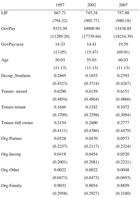
3.3 Data
The data is derived from the Census of Agriculture longitudinal file maintained by USDA-NASS. A subset from census years 1997, 2002, and 2007 is used in this study. This dataset allows the researcher to follow farm operators every 5 years. Tables 1 and 2 report summary statistics of all the variables used in current research. The dependent variable is “land in farm” defined as: total acres of land owned plus land rented in minus land rented out. The variable for government payments1 per acre is in 2007 dollars. This payment
variable is constructed by dividing total receipt of government outlays by “land in farm”. Operator characteristics such as age and indicator variable for primary occupation (“1” if non-farmer and “0” otherwise) are used as regressors. The dataset also allows to control for land tenure status namely: indicator variables for “full owner” (all land in operation is owned), “mixed” (land in operation is owned and rented), and “tenant” (all land in operation is rented in). Furthermore, there is information on the type of business organization namely: indicator variables for “family2”, “partnership organization”,
“incorporated organization”, and “other organization3”.
Level of government payment depends both on the farm size and crop mix, and crop mix is an important determinant of farm size. For example, grain farms receive more payments and are generally larger than vegetable farms, and the resulting positive relationship between farm size and payments is not causal. Thus the sample is confined to farms identifying primary4 crop produced as corn-soybean and wheat in all three census years (based on NAIC codes). Corn and soybeans are aggregated into one commodity because most producers plant these crops on a rotational basis. Separate regressions are estimated for each crop group.
3.4 Panel Data Quantile Regression
Consider a simple setup that consists of exactly two farm size observations for a large sample of farm operators. The standard linear panel-data model can be represented as:
𝑌𝑖,𝑡 = 𝑥𝑖,𝑡′ 𝛽 + 𝑐
𝑖 + 𝑢𝑖,𝑡 (t=1,2; i= 1,2,….n) (3.1),
where 𝑌𝑖,𝑡 is the farm size outcome of operator i at time t, x denotes a vector of observable
explanatory variables, 𝛽 is the vector of parameters of interest, c denotes the unobserved farm operator specific effect, u is the idiosyncratic error term, and n is the number of observations. The standard linear panel setting lends itself to various estimation techniques. The “pure” random effects regression, where farm operator individual effect (c) is uncorrelated with the covariates (x), is implausible in the current application as discussed above. This leaves two remaining estimators, namely, fixed and correlated random effects.
It is well known that fixed effects regression can be consistently estimated using a first differenced regression. However, the conditional expectation is a linear operator whereas the conditional quantile is not5, thus making the standard differencing technique infeasible for quantile applications (Koenker and Hallock (2000)). Furthermore, if the number of waves (t) is small, and the number of observations (i) is large (as in the current study), it leads to what is known as the “incidental parameter problem” – where the number of parameters needed to control for individual specific effect via dummy variables increases with sample size .
In order to overcome the incidental parameters issue, Koenker (2004) proposes a model for fixed-effects quantile regression where the unobserved fixed effect is a location shift on the distribution of the response variable. That is, it is the same for each percentile. However, BDK (2013) have shown in their simulation exercise that Koenker’s (2004)
approach does not perform very well when (c) has a scale effect - a concern for the current application. Furthermore, they show that correlated random effects quantile regression models do not suffer from the incidental parameter problem and perform well even when omitted items have a scale effect on the response variable. BDK (2013) examine two quantile specifications of the correlated random effects estimator. The first was developed