Automatic stance detection on political discourse in Twitter

(1)

on Political Discourse in Twitter

Author:

Elena Zotova

Advisors:

Rodrigo Agerri and German Rigau

Hizkuntzaren Azterketa eta Prozesamendua Language Analysis and Processing

Master’s Thesis

Department: Computer Systems and Languages, University of the Basque Country UP-V/EHU.

Donostia San Sebasti´an September 2019

(2)

(3)

Acknowledgments

I would like to acknowledge my warmest thanks to my supervisors Dr Rodrigo Agerri and Dr German Rigau for their friendly and understanding guidance, constructive comments and ideas. I prepared this thesis living in Madrid, and my supervisors made everything to make our remote meetings, discussions and work convenient and easy, and always helped when I had doubts.

Besides, I wish to thank all the professors in the Master of Language Analysis and Pro-cessing of the University of the Basque Country. It was a pleasure and a big luck for me to meet people such passionate about linguistics, NLP and their native language. I have learned a lot.

I would also wish to express my gratitude to Manuel Nu˜nez, head of department of statistic research in Intercom Strategies, Madrid, where I worked during preparing and writing this master thesis, for his expert advice and permission to use the company’s software for my research.

Also, I would like to thank Francisco Rangel, from PRHLT Research Center, Universitat Polit´ecnica de Val´encia, one of the organizers of Task on Multimodal Stance Detection in Tweets on Catalan #1Oct Referendum in IberEval 2018, who kindly provided the dataset. Finally, I would like to say special thanks to my boyfriend for his support, inspiration, listening to multiple stories about this thesis, and participating in rehearsals of the presen-tation. And thanks to my new friends I have met during my stay in Donostia for fruitful conversations and encouragement.

(4)

(5)

Abstract

The majority of opinion mining tasks in natural language processing (NLP) have been focused on sentiment analysis of texts about products and services while there is comparatively less research on automatic detection of political opinion. Almost all previous research work has been done for English, while this thesis is focused on the automatic detection of stance (whether he or she is favorable or not towards important political topic) from Twitter posts in Catalan, Spanish and English. The main objective of this work is to build and compare automatic stance detection systems using supervised

both classic machine and deep learning techniques. We also study the influence of text normalization and perform experiments with different methods for word representations

such as TF-IDF measures for unigrams, word embeddings, tweet embeddings, and contextual character-based embeddings. We obtain state-of-the-art results in the stance detection task on the IberEval 2018 dataset. Our research shows that text normalization

and feature selection is important for the systems with unigram features, and does not affect the performance when working with word vector representations. Classic methods such as unigrams and SVM classifer still outperform deep learning techniques, but seem to be prone to overfitting. The classifiers trained using word vector representations and the neural network models encoded with contextual character-based vectors show greater

robustness.

Keywords: Text Categorization, Stance Detection, Opinion Mining, Supervised Machine Learning

(6)

(7)

List of Figures

1 Distribution of classes in the Catalan dataset. . . 11

2 Distribution of classes in the Spanish dataset. . . 12

3 The workflow in RapidMiner: the training and evaluating process. . . 14

4 Continuous bag-of-words proposed by Mikolov et al. (2013). . . 16

(10)

(11)

List of Tables

1 Train and test datasets of TW-1O Referendum corpus. . . 10

2 Number of examples per target in the SemEval 2016 English dataset. . . . 13

3 Cross-validation results of TF-IDF+SVM models . . . 24

4 F1 scores for best TF-IDF+SVM models in cross-validation. . . 24

5 Comparison of models for Spanish dataset. . . 25

6 F1 scores for models trained with different parameters evaluated on 10-fold cross-valdation. . . 25

7 Performance of Catalan+Spanish model in cross-validation. . . 26

8 Cross validation results for FastText+SVM models. . . 27

9 F1 scores in cross-validation for FastText+SVM system. . . 28

10 The F1 score of systems trained with Flair architecture. . . 28

11 F1 scores of best models on the training set. . . 29

12 Test performance on TW-1O Referendum corpus for Spanish language. . . 29

13 Test performance on the TW-1O Referendum corpus for Catalan language. 30 14 Comparison of test performance on SemEval 2016 Stance Detection dataset for English language. . . 31

15 Number of incorrectly predicted examples in test datasets. . . 32

16 Number of errors common for the systems. . . 32

17 Error Types over 100 examples . . . 33

18 Confusion matrix on Spanish test set. . . 49

19 Confusion matrix on Catalan test set. . . 49

20 Test performance of the Spanish systems in terms of F1 macro score for 2 classes: AGAINST and FAVOR. . . 50

21 Test performance of the Catalan systems in terms of F1 macro score for 2 classes: AGAINST and FAVOR. . . 50

22 Test performance of the English systems in terms of F1 macro score for 2 classes: AGAINST and FAVOR.. . . 50 23 Most frequent words from Spanish dataset that occur more than 100 times. 51

(12)

(13)

1

Introduction

The importance of Natural Language Processing (NLP) methods for opinion mining grows due to the rapidly increasing amounts of text information produced in Internet by mass media and users in social media. This text data is unstructured, but contains valuable knowledge that may be useful for various purposes. It gives easy and massive access to public feedback about almost every topic of society: services, products, politics and many others; while the classical methods of public opinion such as polls and surveys are expensive and require much more time and human resources. That is why the demand of automatic categorization and opinion mining artificial intelligence algorithms is ever increasing. This information is of big interest for marketers, researchers, and politicians, but also for busi-ness intelligence, government intelligence, decision support systems, political and social researches.

Social media has a great impact in Spain. For example, Spain is one of the top ten most active countries in Twitter. In January 2019 the microblogging service in this country had 6.01 million users1. Furthermore, the discourse on this microblogging platform in Spain is highly politicized. Every political event resonates in posts of social media immediately, and in Twitter more promptly than in other media. All Spanish politicians and politi-cal activists have their Twitter accounts and directly express opinions on many points, provoking heated debates and generating news reports.

Twitter gives access to new information instantly, allowing to share opinions, facts, pictures, videos, and to participate in discussions. Moreover, the analysis of social me-dia content may reveal some insights. For example, an analysis of about 900.000 tweets (Boynton and Jr., 2016) showed that the public in the United Kingdom had already been in favor of Brexit since 2012, and stayed like that until the referendum, but the traditional opinion polls were not able to detect that. In addition, some studies such as Hill et al. (2013); Bovet et al. (2016) affirm that extracted opinions from social media show a strong correlation to the opinions obtained via traditional approaches such as polls and surveys.

Taking this into account, in this thesis we will focus on the stance detection of political discourse in Twitter for three languages: Catalan, Spanish and English. We will examine the stance detection in debates about the Catalonia self-determination Referendum which took place in Catalonia on the 1st of October 2017. The referendum was approved by the Catalan Parliament on September the 6th but was declared illegal by the Spanish Government and prohibited by the Constitutional Court of Spain a few days after. That provoked heated debates between the supporters (”independentistas”) and the opponents (”unionistas”).

Twitter is a source of great amounts of data for text classification and opinion mining which would be impossible to process manually by humans. The data is easy to collect as the platform provides free access to its public API2 (application programming interface) which allows to connect to its databases and receive data in response to specific requests

1_{https://www.statista.com/statistics/242606/number-of-active-twitter-users-in-selected-countries/} 2_{https://developer.twitter.com/en/docs}

(14)

like keyword, period, place etc.

Text classification on social media posts such as tweets is a challenging NLP task. Tweets are very short, up to 240 characters, and there are a lot of messages that contain very few words, specific vocabulary, slang, orthographic mistakes and non-grammatical phrases, emojis, hashtags, images, links, pieces of irony and sarcasm. The same user can write in two or three languages. Twitter message is instant, highly emotional and sometimes difficult to classify even for humans, especially if we only have available a few tweets from some user without context and without connections with other participants of the discussion.

1.1

Stance Detection: Problem Statement

Stance is a way of thinking about some topic, problem, person or object, expressed as a public opinion 3_{. In Natural Language Processing (NLP), stance detection refers to}

automatically predicting whether the author of a given statement is in favor of some topic, event or person (target) or against it. Sometimes a text does not expresses any stance towards the target, in this case the stance is neutral, or absent (Ghanem et al., 2018).

More specifically, the problem is the following. We have a set of tweets and a given target. For instance, the referendum on self-determination of Catalonia in 2017. The task is for the NLP to detect whether the text represents the stance in favor of the target topic or against it (or whether none of them are expressed). Below there are some examples in Spanish from the MultiStanceCat dataset (MultiModal Stance Detection in tweets on Catalan #1Oct Referendum) (Taul´e et al., 2018).

Example 1: Los catalanes que dicen que quieren #democracia (votar en el #refer´endum del #1O), no independencia, mienten.

Translation: The Catalans who say that they want #democracy (to vote on the #referendum of #1O), but not independence, lie.

Stance: AGAINST

According to the task definition, a NLP system for stance detection should classify this sentence taking into account only textual information, without any knowledge about the Twitter user, the thread of the conversation and the connection with other users. Example 1 is relatively “easy”, because the target topic and the attitude to it is explicit. In many cases the stance is expressed indirectly, without naming the topic but mentioning the persons, facts or events related to the topic, as shown by Example 2, for which we need background information to know that the referendum was held on the 1st of October.

Example 2. Me voy a meter en la cama el 30 de septiembre y no voy a salir hasta el 5 o el 6 d octubre #Catalunya #Independencia #1OCT #Hastaelmismisimo

(15)

Translation: I am going to the bed the 30th of September and won’t leave it till the 5th or 6th of October #Catalunya #Independencia #1OCT #Hastaelmis-misimo

Stance: AGAINST

There are some posts which, in isolation, are very difficult or just impossible for humans to deduce whether the statement is against or favor to the Catalan referendum, as it can be seen in Example 3. We can see here the lack of evidence of the attitude to the topic, without the specific hashtag we cannot even guess what it is about. Furthermore, a post may not support any of the controversial points of view, and be “against everything”, like in Example 4.

Example 3: De verdad, no hay mas ciego que el que no quiere ver. #Catalunya #1octubreARV

Translation: Really, there is no more blind one than one who does not want to see. #1octubreARV

Example 4. Vaya desastre de debate. Y vaya politicos que tenemos. Todos. Uff que nivel #1octubreARV

Translation: What a mess the debate is. And what politicians we have. All of them. Uff what a level #1octubreARV

Stance: NEUTRAL

It is considered that stance detection has much in common with the sentiment analysis. In sentiment analysis, systems try to determine whether the polarity of a given text is positive, negative, or neutral. In stance detection, in contrast, systems are to determine if the author says that he/she is against or for some given topic, which may be implicit and difficult to extract from the short text. The difference is that the text may express negative opinion about an entity contained in the text, but one can also conclude that the author is favorable towards the target (a person, an event, an entity or a topic). It means we cannot consider negative sentiment in the message as an equivalent of ”against” stance (Sobhani et al., 2016). Thus Example 5 expresses a negative attitude towards In´es Arrimadas, a Spanish politician while at the same time expressing a favour stance towards the target topic (the referendum).

Example 5: Arrimadassss para de decir tonter´ıas, nos vamos!! #1octL6

Translation: Arrimadassss stop saying nonsense, we are going!! #1octL6

Stance: FAVOR

One more difference between stance and sentiment that stance may be express without using any emotional words. In Example 6 there are not any sentiment words, but it is possible to infer that the author is against of the referendum, because it will cause a big expense for the Catalan government.

(16)

Example 6. #1octl6 Y ... esto quien lo paga?

Translation: #1octl6 And ... who will pay for this?

Stance: AGAINST

Summarizing, automatic stance detection is not a trivial task and present some specific challenges, such as implicit targets, absence of context and complex ways to express stance.

1.2

Research Objectives

In this thesis we focus on building multilingual systems for automatic stance detection on political discourse in Twitter. Our research objectives are the following:

1. To build classification models able to detect stance in a Twitter message towards the topic related to politics using machine learning techniques, exploring different approaches to feature selection.

2. To study the influence of text pre-processing and normalization of social media posts for the stance detection task.

3. To study word and document vector representations and its influence on the perfor-mance of the classification systems for stance detection.

4. To analyze and compare the performance of the systems with the state of the art. 5. To explore the robustness of the stance detection systems across languages, aiming

to develop systems with the ability to generalize across datasets and languages. 6. To analyze the errors of the applied algorithms and propose the ways of improvement

of the classification systems.

1.3

Document Description

The rest of the thesis is organized as follows. In Section 2 we review several state-of-the-art works related to automatic stance detection. We present the main approaches for Spanish, Catalan and English languages. In Section 3 we describe the methodology applied to our research. We present the datasets from the IberEval 2018 (Taul´e et al., 2018) and SemEval 2016 (Mohammad et al., 2016b) shared tasks which are used for training and evaluating the classification models. Also, we describe the algorithms and tools used to undertake our experimentation. In Section 4 we describe the experimental set-up of the work and the different systems built and evaluated. We offer some concluding remarks about the tuning of our systems and provide an error analysis of our system. We finish this master’s thesis in Section 6 with the final conclusion and discussion for future work.

(17)

2

State of the Art

2.1

Opinion Mining, Sentiment Analysis and Stance Detection

With the growing availability and popularity of opinirich textual resources such as on-line review sites, personal blogs and social media, new opportunities and challenges arise as people and organizations use natural language technologies to understand the opinions expressed by others. Sentiment Analysis is the sub-field of Natural Language Processing (NLP) that studies people’s opinions, sentiments, and attitudes towards products, organi-zations, entities or topics. Although several complex emotion categorization models have been proposed in the literature (Russell, 1980; Cambria et al., 2010) most of the Senti-ment Analysis community has assumed a simpler categorization consisting of two variables: subjectivity and polarity. A text is said to be subjective if it conveys an opinion, and objective otherwise. We understandpolarity classification as the task of telling whether a piece of text (document, sentence, phrase or term) expresses a sentiment.

Automatic stance detection is the task of classifying the attitude expressed in a text towards a given target Mohammad et al. (2016b). Stance detection can be viewed as a subtask of Opinion Mining being also closely related to Sentiment Analysis Pang et al. (2008) and Text Classification Aggarwal and Zhai (2012).

There are three levels in the investigation of sentiment analysis: document level, sen-tence level and aspect level.

• The task in the document level is to predict negative, positive or neutral sentiment of the whole document such as article, social media post or user review (Pang et al., 2002; Turney, 2002; Dave et al., 2003). This task can be approached using very well known Text Classification techniques. The problem appears when the document contains opinions of various targets.

• Sentence level is usually related to objectivity classification in order to distinguish subjective, objective o neutral information (Wiebe et al., 1999; Finn et al., 2002). Again this task can be addressed applying Text Classification techniques.

• In the aspect level also known as Aspect Based Sentiment Analysis (ABSA) the goal is to determine the sentiment towards different aspects of the topic, product o service rather than the whole text (Pontiki et al., 2014, 2015; Poria et al., 2016; Pablos et al., 2018). For example, in mobile phone reviews, the speed of the processor and the screen resolution may be estimated with different polarity in the same message: ”the speed is good but the screen is too poor”. ABSA takes into account the different targets of an statement, which makes it similar to stance detection task.

Earlier attempts to computationally assess sentiment in text were based on document classification (Pang et al., 2002; Turney, 2002; Hu and Liu, 2004). As a classification problem, multiple machine learning techniques have been applied to Sentiment Analysis Liu (2012). This task is usually a two-class classification problem (positive vs. negative).

(18)

Sometimes a third class (neutral) is introduced. Because many of them relied on the presence of polar words and/or co-occurrence statistics, a document guarantees to have a fair amount of clues. Also, some sources such as movie reviews provided ready-to-use document level annotations, making it possible to develop the first supervised systems (Pang et al., 2002). Supervised machine learning techniques require gold-standard datasets to be collected and annotated manually by humans for being used as training and testing data for the classifiers.

As for any supervised machine learning classification problem, one of the most impor-tant task is feature engineering. There are several categories of features that have been tried to represent textual examples for opinion mining.

N-grams with different weighting schemes such as frequency and TF-IDF. This approach is successfully used in the majority of text classification tasks. Pang et al. (2002) was the first who categorized movie reviews into positive and negative and showed that the models trained with unigrams as features and Na¨ıve Bayes and Support Vector Machines (SVM) classifiers performed better that other approaches.

Part-of-speech of the words may provide information, for example, adjectives indicate that the speech is more emotional and subjective.

Lexicon based features are sentiment words and phrases are specific entities for express-ing negative or positive sentiments in a text. We know that good, incredible and fantastic

usually used to say something positive and bad, awful and terrible are about something negative. Lexical dictionaries and databases such as WordNet Miller et al.; Qiu et al.; Al-Kabi et al.; Baccianella et al.; San Vicente et al. are used for the feature generation.

Syntactic dependencies generated from dependency parsing are also have been used together with classical features. (Xia and Zong, 2010; Ng et al., 2006)

For classification, a wide range of methods is used, among them statistical models, regressions, support vector machines and recently, deep neural networks.

Unsupervised learning includes lexicon-based approaches, which are difficult for social media due to non-grammatical entities and misspelled words (Taboada et al., 2011; Hu et al., 2013). The approach of Lin and He (2009); Pablos et al. (2018); Shams and Baraani-Dastjerdi (2017) is based on combining topic modelling with Latent Dirichlet Allocation (LDA) and sentiment classification.

Sentiment analysis is highly dependent on the domain, and a model trained on specific dataset may perform poorly on the unseen texts from different domain. Also, there is a lack of well labelled datasets for different targets. Lately, in order to resolve this problem, cross domain sentiment analysis is being addressed. The main goal of this task is transfer the knowledge from labelled data to target data where no labelled or a limited corpus exist. In this scenario the researchers study shared features and relations between the domains (Blitzer et al., 2006; Pan et al., 2010; Li et al., 2009). Now, the main approach is deep learning including recurrent neural networks with attention mechanism (Chen et al., 2012; Glorot et al., 2011; Zhang et al., 2019). Supervised deep learning systems use to require large volumes of manually annotated data (Chen et al., 2017; Araque et al., 2017) although very recent unsupervised contextual word embeddings such as BERT Devlin et al. (2019) pre-trained on very large corpora are obtaining state-of-the art results fine tuning

(19)

the model with very small training data.

2.2

English Language

Stance detection as a subtask of opinion mining and sentiment analysis is a relatively new research area in NLP. From the beginning, the main approach for stance classification has been supervised machine learning. Initial works mainly focused on congressional debates (Thomas et al., 2006) or debates in online forums (Somasundaran and Wiebe, 2009; Mu-rakami and Raymond, 2010; Anand et al., 2011; Walker et al., 2012; Hasan and Ng, 2014; Sridhar et al., 2014). These domains are specific because the gold labels can easily be obtained. For instance, in Sridhar et al. (2014) approach the authors collect posts from various authors from social media debate sites and forums, where all posts are connected as dialogues or responses to the main post of the discussion. The posts are linked to one another by agreement or rebuttal links and are already ”labelled” for stance, either

PRO or CONTRA. Main approaches for debate stance detection have used sentiment and argument lexicons, statistical measures and counts, n-grams, repeated punctuation, part-of-speech tagging, syntactic dependencies and may others (Wang et al., 2019).

Research on Twitter posts started in 2014, and presented a new challenge to the NLP community since tweets are short, informal, full of misspellings, shortenings, slang and emoticons, and are produced in large amount with great velocity. Researchers Rajadesingan and Liu (2014) were the first who determined stance at user level. They assumed that if many users retweet a particular pair of tweets in a short time, then this is likely that this pair of tweets had something in common and share the same opinion on the topic.

The first Stance Detection in Tweets task4 was presented in 2016 as a part of SemEval challenge organized by the National Research Council Canada. The task aimed to detect stance from single tweets, without taking into account conversational structure of online debates and information about authors. The SemEval competition included two subtasks. Task A was formulated as follows: “given a tweet text and a target entity (person, or-ganization, movement, policy, etc.), automatic natural language systems must determine whether the tweeter is in favor of the given target, against the given target, or whether neither inference is likely” Mohammad et al. (2016b). In Task B the goal was to detect stance in relation of unseen target. The organizers of the challenge also prepared a new dataset which consisted of 4.000 tweets in English corresponding to five stance targets, such as abortions, religion, climate changes, etc., and was annotated both with stance and sentiment labels.

The baseline system designed for the challenge built by the organizers obtained the best results. This baseline system outperformed the submissions from all 19 teams that had participated in the competition. The features used in the system were the following: word and character n-grams, average word embeddings, and sentiment features. A su-pervised system was trained using a support vector machine classifier (Mohammad et al., 2016b). Other approaches were based on convolutional neural networks (CNN) (Wan Wei,

(20)

2016; Vijayaraghavan et al., 2016), recurrent neural network (RNN) (Zarrella and Marsh, 2016), ensemble model (Liu et al., 2016), maximum entropy classifier and domain dictio-naries (Krejzl and Steinberger, 2016), etc. Most of the participants used standard text classification features such as word and sentence vector embeddings and n-grams.

The state of the art in stance detection on the SemEval 2016 dataset currently is hierarchical attention based neural model proposed by Sun et al. (2018). In this approach, implemented after the SemEval task, the document is represented under the influence of linguistic features. A linguistic attention mechanism (Kim et al., 2017) is used to learn the correlations between document representation and different linguistic features. The linguistic features are sentimental word sequence, dependency-based features and argument sentence. The document level representation is based on pre-trained word2vec vectors. Documents and linguistic feature sets are encoded with various LSTMs.

In Task B of the SemEval task the stance targets not always present in the message and no training data is available to test the targets. For example, a tweet with positive stance towards Donald Trump is also a negative stance towards Hillary Clinton as implicit target. The best system was proposed by Augenstein et al. (2016). The novel approach is focused on target-dependent representations of tweets. The experiment is done with conditional encoding with neural architecture (LSTM), which builds a representation of the tweet that is dependent on the target. The researchers combine the vector representation on the target and the vector representation of the tweet, and predict stance for target-tweet pair. They also train word2vec model on a large amount of tweets containing targets.

2.3

Spanish and Catalan Languages

We should note that all mentioned works were implemented on the English dataset. The first challenge in stance detection in Spanish and Catalan languages was carried out in IberEval 20175, the 2nd Workshop on the Evaluation of Human Language Technologies for Iberian languages, during the SEPLN 2017 conference. The organizers of the workshop offered a task related to automatic stance detection and presented a dataset of tweets in Spanish and Catalan (Bosco et al., 2016; Mariona Taule and Patt´ı, 2017) where the independence of Catalonia is discussed6_{. The authors of the best system of the task do}

experiments with different types of features such as part of speech, lemmas, hashtags, length of tweets etc., and a set of classifiers (Lai et al., 2017).

In 2018, the third IberEval 2018 workshop7 co-located with the SEPLN 2018 confer-ence also included a stance detection task. The aim of the MultiModal Stance Detection in tweets on Catalan #1Oct Referendum task at IberEval 2018 (MultiStanceCat) was to detect the authors stances–in favor, against or neutral– with respect to the Catalan Oc-tober, 1 Referendum (2017) in tweets written in Spanish and Catalan from a multimodal perspective. The dataset also contained images from the given tweets (Taul´e et al., 2018).

5_{http://nlp.uned.es/IberEval-2017/index.php/} 6_{http://stel.ub.edu/Stance-IberEval2017/data.html} 7_{http://www.autoritas.net/MultiStanceCat-IberEval-2018/}

(21)

The best results on this task were obtained by a team from the Carlos III University (LABDA). They presented a system based on simple bag-of-words approach with TF-IDF vectorization (Segura-Bedmar, 2018). They evaluated several of the most broadly used classifiers. The colleagues do not report anything about pre-processing of the text. They only try to train the model using single tweets with context and without it. This baseline obtained F1 score=0.28 in test evaluation on Spanish dataset.

For the Catalan, the Casacufans team approached the task using texts and images. They used hashing vectorizing from the Scikit-learn toolkit to pre-process and represent texts, and they use linear SVM to train the model. With respect to images, the participants trained a Convolutional Neural Network to detect Spanish or Catalan flags. As report the organizers of the task, the authors did not provide a working note explaining their approach in details (Taul´e et al., 2018).

The approach of the Polytechnic University of Valencia team (CriCa) (Cuquerella and Rodr´ıguez, 2018) was to combine datasets of Spanish and Catalan to create a larger corpus and make it more balanced. They did various experiments. The baseline was simple tokenizing and training a Linear SVM classifier. The first model was with stemming with different length of the stem (three, four and five characters) and removing fixed number of characters from the ending of the word. Since Spanish and Catalan share many words, especially, stemming helped to generalize. Additionaly, and some tweets also contain texts in both languages.

It should be underlined that in the Spanish and Catalan datasets, there is still a wide margin to test state of the art NLP approaches to build better stance classifications systems.

(22)

3

Methodology

For our investigation we need 1) annotated corpora for training supervised systems and 2) tools for building automatic stance recognition systems. The experimentation has been undertaken using the following tools: RapidMiner software and Scikit Learn8 (Pedregosa et al., 2011) to train SVM supervised machine learning models, Gensim9 _{( ˇ}_Reh˚_{uˇrek and}

Sojka, 2010) for working with word embeddings and Flair10 _{(Akbik et al., 2018) as a deep}

learning platform to train Recursive Neural Networks for stance detection.

3.1

Datasets

In the experiments we use three datasets: in Spanish, Catalan and English. The Spanish and Catalan datasets first were presented in IberEval shared task in 2018 (Taul´e et al., 2018) and the English dataset was presented within the 2016 SemEval shared task (Mohammad et al., 2016b).

3.1.1 TW-1O Referendum corpus, IberEval 2018

The datasets in Spanish and Catalan were collected as follows. The organizers used the #1oct, #1O, #1oct2017 and #1octl6 hashtags to select the tweets to be included in the TW-1O Referendum corpus11 _(Taul´_{e et al., 2018). These hashtags were the most widely}

used (especially the first two) in the debate on the right to hold a unilateral referendum on Catalan independence from Spain. A total of 87,449 tweets in Catalan and 132,699 tweets in Spanish were collected from September, 20 to the day before the Referendum was held (2017 September, 30). From this data the TW-1O Referendum corpus was built. The final consists of 11,398 tweets: 5,853 written in Catalan (the TW-1OReferendum CA corpus) and 5,545 in Spanish (the TW-1OReferendum ES corpus).

Language Train Test Total

Catalan 4684 1169 5853 Spanish 4437 1108 5545

Table 1: Train and test datasets of TW-1O Referendum corpus.

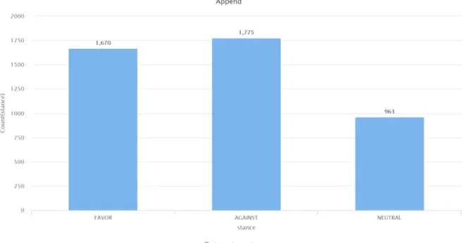
Each tweet is provided in context, which is formed by its previous and next tweets from the user’s Twitter timeline, also including any pictures that the tweets may contain. Eighty percent of the corpus was used for training purposes, while the remaining twenty percent was used for testing. The Spanish part of the corpus is relatively well balanced, as we shown by Figure 2, while the Catalan set is hugely skewed towards the FAVOR class, as illustrated by Figure 1.

8_{https://scikit-learn.org}

9_{https://radimrehurek.com/gensim/}

10_{https://github.com/zalandoresearch/flair}

(23)

Figure 1: Distribution of classes in the Catalan dataset. Here we can see some tweet examples from the corpus.

1. Tweet: Res ni ning´u, ens aturar´a #Votarem #DretaDecidir #1Oct #Catalun-yaLliure #defensemlademocracia http://t.co/PgVLYH8AgN

Language: Catalan Stance: FAVOR

Translation: Nothing and nobody will stop us #Votarem #DretaDecidir #1Oct #CatalunyaLliure #defensemlademocracia http://t.co/PgVLYH8AgN

2. Tweet: Mientras tanto en #España se espera una REPRESION para todo público este #1Oct Tan democráticos ellos... https://t.co/gw7QIfrjHk

Language: Spanish Stance: FAVOR

Translation: Meanwhile in #Espa˜na a REPRESSION is expected by the general public this #1Oct Very democratic them... https://t.co/gw7QIfrjHk

3. Tweet: Adeu #1octubreARV #1octubrenovotare http://t.co/x3dXO3v7np

Language: Catalan Stance: AGAINST

(24)

Figure 2: Distribution of classes in the Spanish dataset.

4. Tweet: M´as q votos creo q estais usando personas jugando con sus sen-timientos SABIAIS q el #1Oct ES ILEGAL https://t.co/1SJcwn7LHd

Language: Spanish Stance: AGAINST

Translation: You know that more than votes you are using persons playing with their sentiments YOU KNOW that the #1Oct IS ILLEGAL https://t.co/1SJcwn7LHd

5. Tweet: Voteu! #1Oct Crees que la respuesta del Estado al desaf´ıo indepen-dentista catal´an est´a siendo adecuada? https://t.co/LlZrkd20gh v´ıa @20m

Language: Catalan+Spanish Stance: NEUTRAL

Translation: Vote! #1Oct Do you think that the States response to the Catalan pro+independence challenge is appropriate? https://t.co/LlZrkd20gh va @20m

6. Tweet: Necesito alguien con quien comentar #1octL6

Language: Spanish Stance: NEUTRAL

(25)

3.1.2 SemEval 2016

The dataset in English12_{was presented at the Stance Detection task organized at SemEval}

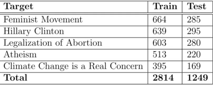
2016 (Mohammad et al., 2016b). It consists of tweets labeled for both stance and sentiment (Mohammad et al., 2016a). We do not use the sentiment labels available in this dataset in order to keep the same experimental setup as for the Spanish and Catalan datasets, for which not sentiment annotations are available. In the supervised track, more than 4,000 tweets are annotated with respect to five targets: “Atheism”, “Climate Change is a Real Concern”, “Feminist Movement”, “Hillary Clinton”, and “Legalization of Abortion”. For each target, the annotated tweets were ordered by their timestamps. The first 70 percent of the tweets formed the training set and the last 30 percent were reserved for the test set. To prepare the dataset, the organizers collected 2 million tweets containing favor, against and ambiguous hashtags for the selected targets. Each of the tweets was also annotated for whether the target of opinion expressed in the tweet is the same as the given target of interest. The organizers made a small list of query hashtags and split them into three categories: favor, against and ambiguous. Later, the hashtags were removed from the corpus. As only tweets with hashtags in the end of the tweet were used, the grammar and syntactic structure are kept. The authors organized a questionnaire and crowdsourcing setup for annotating stance. Each tweet was annotated by eight respondents (Mohammad et al., 2016a).

Target Train Test

Feminist Movement 664 285

Hillary Clinton 639 295

Legalization of Abortion 603 280

Atheism 513 220

Climate Change is a Real Concern 395 169

Total 2814 1249

Table 2: Number of examples per target in the SemEval 2016 English dataset. Some examples from SemEval 2016 dataset follow.

1. Tweet: I still remember the days when I prayed God for strength.. then sud-denly God gave me difficulties to make me strong. Thank you God! #SemST

Target: Atheism Stance: AGAINST

2. Tweet: @PH4NT4M @MarcusChoOo @CheyenneWYN women. The term is women. Misogynist! #SemST

Target: Feminist Movement Stance: FAVOR

(26)

3.2

Tools and Algorithms

3.2.1 RapidMiner

The first part of our experiments was done with RapidMiner13_{, a data science software}

platform that provides an integrated environment for text mining, machine learning, and predictive analytics. It is suitable for commercial applications as well as for research, education, training, and prototyping. The software supports all steps of the machine learning process including data preparation, results visualization, model validation and optimization (Hofmann Markus, 2013).

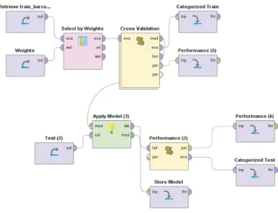
Figure 3: The workflow in RapidMiner: the training and evaluating process.

RapidMiner provides many al-gorithms for supervised learning and clustering, including exten-sions for working with WEKA, Word2Vec, Keras, etc., allowing to build neural networks, prepro-cessing text (tokenize, apply stop-words etc) and encoding of regu-lar expressions. It allows to pro-cess data in various formats, such as CSV, Excel or XML (except JSON). It allows to execute any type of Python or R scripts. It makes the software flexible and suitable for many basic tasks in text mining. RapidMiner is de-veloped on an open core model. The RapidMiner Studio Free Edi-tion is limited to one logical pro-cessor and 10.000 data rows.

The main concepts of RapidMiner are:

• process – a workflow where a special task is done;

• operator – a function, for example the Process documents operator that executes some operations for text processing, or the Cross Validation that executes a cross validation function over a selected estimator. An operator placed into a process may be nested which means that an operator may execute some more subprocesses inside the main process;

• example set – data in a specific format of the application. It can be visualized as a table, or graphics, or statistics. One example is a row. Any example set may be exported to CSV, TXT or XLS format;

(27)

• attribute – a variable, in the Example set it is a column.

In Figure 3 we provide an example of a process of training and testing a model. Datasets are connected to a classifier and then to the model, the Cross Validation operator is nested, and inside there are some more operators, such as a Classifier and Performance. The output of the process is saved as an example set with new attributes-prediction. It also contains the performance scores and the model stored as objects in RapidMiner format. All the text data can be exported to a table or text files.

3.2.2 Word Vector Representations

Vector representations of words, characters or documents, also known as ”embeddings” is a technique for creating language models in continuous real valued representations. We use the following types of vector representations in our experiments:

• Static word embeddings: the most well-known are word2vec (Mikolov et al., 2013), GloVe (Pennington et al., 2014), and FastText (Joulin et al., 2017). They are pre-trained over large corpora and are able to capture semantic and syntactic similarities based on co-ocurrences.

• Character-level embeddings (Lample et al., 2016; Ma and Hovy, 2016), which are trained during the learning process on specific data to capture subword features.

• Contextual string embeddings such as Flair (Akbik et al., 2018) which is an embed-ding for a string of characters in a context.

We use pre-trained FastText and Flair contextual string embeddings as a method of word vector representation. Since Catalan is a less-resourced language, there are not so many NLP resources for its processing. However, FastText provide word vector models trained on Common Crawl14 _{and Wikipedia corpora using a Continuous Bag-of-Words}

(CBOW) architecture with position-weights and 300 dimensions. The Fastext models for Spanish, Catalan and English based on Common Crawl contain around 2 million words each.

The CBOW architecture used in Fasttext was (see Figure 4 first proposed as part of the Word2vec model (Mikolov et al., 2013). Originally there were two architectures implemented in Word2vec: CBOW and skip-gram. CBOW is a bag-of-words model because the order of words in the context does not influence the prediction, but it uses continuous distributed representation of the context. In other words, the CBOW architecture predicts the current word from context words not paying attention to their order. According to the authors, CBOW model is faster then skip-gram. Most importantly, the FastText model is capable of building word vectors for words that do not appear in the vocabulary of the model, i.e. they were not presented in the training set for this model.

(28)

In order to produce vectors for out-of-vocabulary words, such as proper names and misspelled words, FastText word vectors are built from vectors of substrings of characters which are character n-grams of length 5, a window of size 5 and 10 negatives (Grave et al., 2018). In order to do so, FastText averages the vector representation of its character n-grams. However, it fails in vectorizing totally non-grammatical entities that the model has never seen. It means that the accurate pre-processing of the text is important.

Figure 4: Continuous bag-of-words proposed by Mikolov et al. (2013). Flair contextual string embeddings are based on

neural language modeling that allows language to be modeled as distributions over sequences of char-acters instead of words. According to the authors, “this type of embeddings is trained without any ex-plicit notion of words and thus fundamentally model words as sequences of characters, and are contextu-alized by their surrounding text, meaning that the same word will have different embeddings depending on its contextual use” (Akbik et al., 2018). These embeddings are pre-trained on very large unlabeled corpora and are able to capture semantic meaning in context and therefore produce different embeddings for ambiguous words depending on their usage. Since Flair embeddings represent words and context as se-quences of characters, it handles better misspelled and rare words, and is able to detect subword struc-tures and morphology. The authors admit that “by learning to predict the next character on the basis of previous characters, such models capture semantic

and syntactic properties: even though trained without an explicit notion of word and sen-tence boundaries, they have been shown to generate grammatically correct text, including words, subclauses, quotes and sentences” (Akbik et al., 2018).

3.2.3 Classifier: Support Vector Machines

For the experiments with classic machine learning algorithms we selected Support Vector Machines (SVM) classifier (Cortes and Vapnik, 1995) which is implemented in both the RapidMiner and scikit-learn toolkits. SVM is a non-probabilistic linear classifier. The main advantage of SVM method is that it is robust to high dimensionality and sparsity of the feature vectors. It was proven that it is one of the most efficient learning methods for text classification because texts usually have a large number of features and not many of them are totally irrelevant. Also, text classification problems are linearly separable (Joachims, 1998).

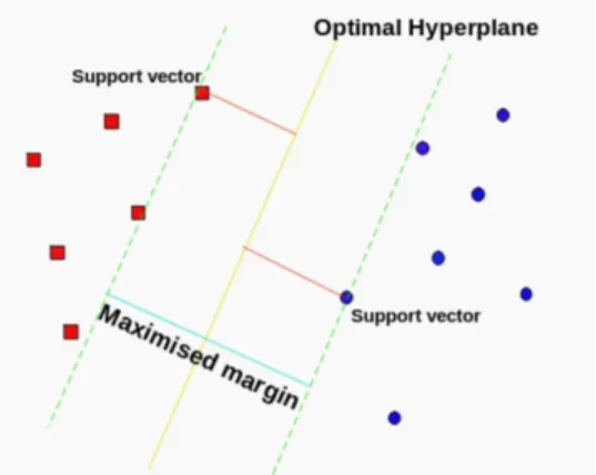
SVM tries to find a hyperplane, which is a separating line, between data of two (or more) classes (The scheme is in the Figure 5). Then the algorithm finds a support vector in such a way that its points are the closest to the line dividing the two classes. The

(29)

distance between the hyperplane and the support vectors is computed; this is functional margin.

The hyperplane that has the largest distance to the nearest training-data point of any class separates the data in the best way. The larger the margin, the lower is the generalization error of the classifier (Hastie et al., 2001). With the appropriate kernel function, SVMs can be used to learn radial basics function (RBF) networks, polynomial classifiers, and three-layer sigmoid neural nets (Joachims, 1998).

Figure 5: The hyperplane of SVM. The SVM learner has various hyper-parameters

to be set, such as kernel type, SVM type, C, gamma, and some more. Hyper-parameters are those which cannot be obtained during the learning process and should be set before it. We select C-SVC type with RBF kernel type. C-SVC type handles multi-class classification according to a one-vs-one scheme. RBF kernel performs well in the models where relation between class labels and features is nonlinear. In the experiment of Joachims (1998), RBF kernel shows slightly better performance than polynomial.

Two most important parameters which impact the accuracy of the model are gamma and C. As explained in the scikit-learn documentation15_{, the}

gamma parameter defines how far the influence of a single training example reaches, with low values meaning far and high values meaning close. The gamma parameters are the inverse of the radius of influence of samples selected by the model as support vectors. The C parameter is used to balance correct classification of training examples against maxi-mization of the decision functions margin. For larger values of C, a smaller margin will be accepted if the decision function is better at classifying all training points correctly. A lower C will encourage a larger margin, therefore a simpler decision function, but the training accuracy will be lower. In other words, C behaves as a regularization parameter in the SVM. Setting a too large C parameter may result in overfitting.

3.2.4 Neural Networks and Flair library

Neural networks and contextual character embeddings are currently obtaining best results in many Natural Language Processing (NLP) tasks. A new framework, presented in late 2018, Flair library 16 _{provides an environment for building classification models based}

on neural networks. It is a Python library which allows to apply NLP models to many tasks, such as named entity recognition (NER), part-of-speech tagging (PoS), word sense disambiguation, and text classification. In sequence labelling tasks, Flair obtained best results for a number of public benchmarks such as PoS tagging and NER (Akbik et al., 2018). It is multilingual system and contains models for some less-resourced languages,

15_{https://scikit-learn.org/stable/auto_examples/svm/plot_rbf_parameters.html} 16_{https://github.com/zalandoresearch/flair}

(30)

such as Catalan. Flair has simple interfaces for combining different word and document embeddings. The framework is based directly on Pytorch, making it easy to train the models and experiment with new approaches. The library allows to prepare the text corpus, calculate the vector representations and build statistical models with recurrent neural networks.

Flair models allow to combine different types of embeddings by concatenating each em-bedding vector to form the final word vectors in a stack. For instance, stacked emem-beddings may mix FastText static word embeddings and Flair contextual character embeddings, or Flair with ELMo contextual embeddings (Peters et al., 2018). According to experiments done by the authors of Flair, in many configurations it may be beneficial to combine the Flair embeddings with static word embeddings to add potentially greater latent word-level semantics.

Flair architecture for text classification is based on a BiLSTM which is a type of re-current neural network (RNN) (Schuster et al., 1997). RNNs are capable of using internal states, so-called memory, to process sequences of input, building the network on all previ-ously seen inputs, which allows to take into account the context of a sentence. Moreover, the value of each hidden layer unit also depends on its previous state, so the word order and the character order are also considered.

The LSTM architecture (Hochreiter and Schmidhuber, 1997) is widely used in NLP tasks and shows state-of-the-art results. However, to achieve this, it requires the selection and optimization of many hyper-parameters (Reimers and Gurevych, 2017). Flair includes a wrapper for tuning the neural network with the hyper-parameter selection tool Hyper-opt17 (Bergstra et al., 2013). Basically, it is a grid search over the hyper-parameters of the neural net and the number of combinations grows exponentially with the number of parameters set. This step is the most time consuming experimentation stage, and in our case can occupy up to 20-30 hours depending on the computing power of the machine and the number of combinations and it is recommendable to execute it on GPU accelerated hardware. We tune the following hyper-parameters:

• Hidden size: the size of LSTM hidden states.

• Dropout set in range 0.0-0.5: a parameter that prevents overfitting for neural net-works (Srivastava et al., 2014).

• RNN layers: 1 or 2 layers.

• RNN type: The type of activation function is Rectified Linear Unit (ReLU) (Nair and Hinton, 2010). The activation function is necessary to normalize the output values of the network and make them statistically balanced. The ReLU function is linear for all positive values, and zero for all negative values.

• Learning rate set in range: 0.05, 0.1, 0.15, 0.2. The deep neural network is updated by stochastic gradient descent (SGD) and the parameters (weights) are updated like

(31)

this: weight = existing weight - learning rate * gradient. The gradient takes into account a loss function that aims to measure inconsistency between the true label and predicted label. When the loss decreases, the accuracy of the prediction increases. Too small a learning rate will make a training algorithm converge slowly while too large a learning rate will make the training algorithm diverge (Bengio, 2012).

• Mini batch size: 16, 32 examples. Mini batch is a subset of training data to calculate the SGD.

• Max epochs: Epoch is one run of the neural network through the entire training set. Set to 100.

• Number of evaluations: 100.

Also, we trained our models selecting a stacked embedding configuration consisting of FastText Common Crawl and Flair contextual character embeddings.

3.3

Evaluation Metrics

There are various metrics for the evaluation of performance of the classification models: accuracy, precision, recall and F1 scores. Accuracy is the proportion of correctly classified documents with respect to the total number of documents. We do not use the accuracy score as an evaluation method because in unbalanced datasets the accuracy may be very high. However, this does not show that the classification model performs well.

Precision is the fraction of the correct documents (true positive) among the documents identified as positive (true positive and false positive).

P recision= tp

tp+tn

Recall is the percentage of the correct documents (true positive) among all the real positive documents (true positive and false negative).

Recall = tp

tp+f n

F1 score is the harmonic mean of precision and recall. The formula of F1 is the following:

F1 = 2P recision×Recall

P recision+Recall

For evaluating models in the cross-validation step, we use F1 macro-average for all three classes. F1 score macro-average is calculated as F1 metric for each label and their unweighted mean value. This does not take imbalanced data into account. In multi-class classification, macro-average F1 treats all classes equally while F1 micro-average favours the more populated classes (Sokolova and Lapalme, 2009).

(32)

The organizers of Semeval 2016 and IberEval 2018 used the macro-average score of two classes: F1 score (FAVOR) and F1 score (AGAINST), as the bottom-line evaluation metric. The F1 score of NEUTRAL (NONE) class is not taken into account. They provided a Perl script18 _{that calculate the final F-score with this formula:}

F1avg =

F1f avor+F1against

2

The same metric to evaluate the performance when testing of the experiments is applied.

(33)

4

Experiments

Our main goal is to experiment on detecting stance in Spanish and Catalan datasets, and then investigate the robustness of the various models by applying them to the English dataset. The experimental work was organized in three different setups:

1. TF-IDF vectorization with a SVM classifier.

2. Vector representation of tweets with FastText models and SVM classifier.

3. Stacked Flair and FastText vector representation of words to train a neural network (BiLSTM).

4.1

Pre-processing and Normalization

The first step is to perform text pre-processing. Since each tweet in the Catalan and Spanish data is given in context, with the previous and the next tweet, we use them to enrich the text information. We concatenate all three tweets to one document, so the number of words increases and the weight of each token in a tweet is more representative. We try to perform exhaustive text normalization. Normalization is a process of putting words to standard forms, which reduces irrelevant and noisy information. In our case it helps to reduce the number of features for TF-IDF feature representation and to raise the number of words that correspond with the vocabulary of pre-trained models. First, we clean the text from punctuation, remove mentions starting with “@”, “RT”, URLs and numbers. All the words of the corpus were converted to lowercase.

Another part of text normalization is lemmatization, the task of determining that two words have the same root, despite their differences. For example, the Spanish words voy,

iba and ir´e are forms of the verb ir (to go). One Spanish verb has 55 forms, including gerunds and participles, and they may be totally different in spelling. Lemmatization maps all forms to the same initial form–infinitive for verbs or singular masculine form for nouns and adjectives–also called dictionary form. This process is essential for languages such as Spanish and Catalan but not so important for English (Jurafsky and Martin, 2018). The most sophisticated methods of lemmatization use full morphological analysis and POS tagging. In our system, we simplified the task up to replacing the word form with its lemma without analysis. A simple Python function uses a dictionary19 with word forms (values) and their lemmas (keys). It takes each word of a phrase, checks if it is in the values of the dictionary and replaces it with the key of the dictionary. If a word is not in the dictionary, for example if it is a named entity or incorrectly spelled word, the program does not perform any lemmatization.

This method is not accurate, and it is not capable to resolve ambiguities. This means that, for instance, the prepositionpara (for) and the verbpara (to stop) will be mapped to the same lemma, namely, parar (stop). Also it can not handle named entities, especially

(34)

Spanish and Catalan surnames, for example, Ada Colau is converted to ada colar. To reduce the error rate, we manually edited the list of lemmas, and deleted the less frequent ambiguous words. In any case, our experiments showed that this kind of lemmatization reduces dramatically the number of features without loss of semantic information and helps in general to improve results. In addition, it allows to deal with some unseen words. For example, if the word yendo (going) does not appear in the training corpus but another form of its lemma does, then both words will be recognized as having the same lemma, namely, the Spanish verb ir (to go).

Tokenization is the task of segmenting the text into instances such as characters, words, phrases. We split the tweets by white space which allows to keep all the words with hy-phens, and other special symbols. Next, stopwords (auxiliary verbs, prepositions, articles, pronouns and the most frequent words) and words shorter than three characters are re-moved, usually this kind of words do not contain any relevant information.

The next step is normalization of orthography, which is simple replacing repeated letters with one, all vocals and the most frequent consonants, such ass, z, h, m, j etc, and replacing common shortened words to normal form. We do not touch letters that can be double in Spanish and Catalan: t, l, r. The result is like following: holaaaaaaa is converted tohola,

q is converted toque. We also replace all letters with diacritics with simple ones to reduce the number of tokens in the TF-IDF way of vectorization. The replacement is done with regular expressions.

4.2

TF-IDF+SVM

The first experimental setup uses a TF-IDF (Term Frequency times Inverse Document Fre-quency) (Jones, 1972) representation of features extracted from the corpus. This approach is similar to bag-of-words where instead of word frequency the TF-IDF measure is used.

TF-IDF weighting scheme is broadly used for document and text classification, infor-mation retrieval and topic modelling. The goal of using of TF-IDF measure is to reduce the impact of words that occur too frequently in a given corpus as they are less informative than features that occur in a small part of the training corpus. The TF-IDF is the product of two statistic metrics, term frequency and inverse document frequency. It is computed as follows:

wi,j =tfi,j×log

N dfi

Where:

tfi,j= number of occurences of i in j,

dfi = number of documents containing i,

N=total number of documents

Term frequency is the number of times term appears in a document divided on total number of terms in the document (Luhn, 1957). Inverse document frequency represents the weight of the less frequent words in all documents. Thus, IDF is log scaled relation between the total number of documents and the number of documents with a given term. It gives a

(35)

higher weight to words that are not that frequent in the documents. The idea is that terms that occur too frequently in every document are not as helpful for this task because it does not allow to detect the most meaningful words present in the documents. The more rarely a word occurs in the corpus, the higher it is its IDF score (Jurafsky and Martin, 2018).

We calculate the TF-IDF scores for all unigrams in the training corpus and obtain a document-feature matrix with 13,488 features in Spanish corpus, 11,882 features and Catalan corpus and 1,249 for the English data. The number of features equals the size of the vocabulary of the dataset and represents the dimensionality of the document vector. It is extremely sparse, since the documents contains about 20-30 words. So, our task is to reduce the dimensionality of the vector.

4.2.1 Feature Selection

Before training the model we decide what kind of features could be most useful. The goal of the feature selection process is to identify the most relevant features and discard redundant information. Irrelevant features provide almost zero useful information about the dataset, these can be words that occurs in all classes with the same frequency. Feature selection may affect significantly the performance of the classification model reducing overfitting, training time and improving accuracy.

We use the Information Gain method for feature selection, which is a term from infor-mation theory (Cover and Thomas, 2006). In machine learning, this measure provides a way to calculate the mutual information between the features and the classification classes. According to Aggarwal (2012), mutual information “is defined on the basis of the level of co-occurrence between the class and word”. In other words, it represents the predictive power of each feature, and measures the number of bits of information obtained for pre-diction of a class in terms of presence or absence of a feature in a document. It is a filter method that selects features by ranking them with correlation coefficients (Guyon Isabelle, 2003). The information gain scores show how common is the feature in a target class, for example the words that occurs mainly in tweets labelled as FAVOR stance and almost never in AGAINST stance, are very informative and ranked highly.

We understand that in text classifications the most irrelevant features such as stopwords and short words removed mostly before the creating the document-feature matrix. Never-theless, our experiments show that there Information Gain produces a small improvement of the performance. We give more details in Subsection 4.2.2, Table 5. All the weights are normalized and all the features ranked from one to zero. We then select those features that are scored larger than zero.

4.2.2 Spanish, Catalan and English models

We train a classification model via 10-fold cross validation on the training set using the LibSVM learner (Fan et al., 2005) implemented in RapidMiner. The LibSVM learner allows to apply SVM algorithm for a multiclass problem.

(36)

data within estimators, they must be selected before the training process starts. In order to do this, we perform hyper-parameter optimisation by search. The goal of grid-search is to find the optimal hyper-parameters of a model. It is an exhaustive grid-search through a manually specified subset of parameters of a classifier. Exhaustive search is an algorithm that examines all possible combinations of parameters and checks if they fulfil the condition. During the grid-search SVM models with different parameters are built and estimated by performance metrics, accuracy, precision, and recall and measured by 5-fold cross-validation on the training set.

To reduce the cost of the grid-search process, we select two parameters of SVM classifier only, C and gamma. In total, there were 121 combination of the parameters. The following final hyper-parameters were chosen after grid-search. For Spanish: C=700, gamma=0.3; for Catalan: C=100, gamma=0,4507. The kernel is RBF.

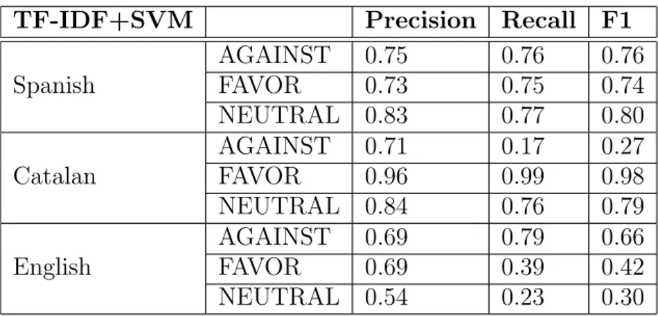
After selecting the best parameters we estimate the classification models via 10-fold cross-validation. For the English data, we train five models according to the target and calculate the average for each metric. We obtain the following results for the best models selected according to the cross validation F1 scores (Table 3, Table 4):

TF-IDF+SVM Precision Recall F1

Spanish AGAINST 0.75 0.76 0.76 FAVOR 0.73 0.75 0.74 NEUTRAL 0.83 0.77 0.80 Catalan AGAINST 0.71 0.17 0.27 FAVOR 0.96 0.99 0.98 NEUTRAL 0.84 0.76 0.79 English AGAINST 0.69 0.79 0.66 FAVOR 0.69 0.39 0.42 NEUTRAL 0.54 0.23 0.30

Table 3: Cross-validation results of TF-IDF+SVM models

Dataset F1 2 classes F1 3 classes

Spanish 0.75 0.77

Catalan 0.62 0.68

English 0.54 0.46

Table 4: F1 scores for best TF-IDF+SVM models in cross-validation.

The worst performance is for the English dataset. We think that this might due to the small amount of training examples. For the Catalan model the result is predictably worse because of the imbalanced dataset where the AGAINST class is very scarcely represented. We also trained the Spanish models in order to perform an ablation test to check which components of our system have a bigger impact in performance.

(37)

Our experiments show (Tables 5 and 6) that the grid-search optimisation of hyper-parameters strongly affects the accuracy of the model. Training the SVM model with default parameters (C=1, gamma=0), the F1 score dropped dramatically to 0.29. The other parts of the system do not impact the result so strongly, but the accuracy of the model still deteriorates.

Spanish Dataset Class Precision Recall F1

Lemmas+Feature selection

AGAINST 0.75 0.76 0.76

FAVOR 0.73 0.75 0.74

NEUTRAL 0.83 0.77 0.80

Without grid search

AGAINST 0.40 1 0.57 FAVOR 0 0 0 NEUTRAL 0 0 0 Without pre-processing AGAINST 0.54 0.93 0.69 FAVOR 0.73 0.51 0.60 NEUTRAL 0.97 0.20 0.34

Without feature selection

AGAINST 0.70 0.73 0.72

FAVOR 0.66 0.75 0.70

NEUTRAL 0.66 0.46 0.54

Table 5: Comparison of models for Spanish dataset.

Model for Spanish Dataset F1 2 classes F1 3 classes Lemmas+Feature selection 0.75 0.77

Without grid search 0.29 0.19

Without preprocessing 0.65 0.54

Without feature selection 0.71 0.65

Table 6: F1 scores for models trained with different parameters evaluated on 10-fold cross-valdation.

We can conclude that text pre-processing and proper feature selection is crucial for good results in the stance detection tasks. Reducing the number of features helps to generalize and minimize the cost in time of training and predicting.

4.2.3 Catalan and Spanish Combined

We performed an additional experiment training on a mixed dataset of Spanish and Catalan examples. Catalan and Spanish languages are grammatically similar and share some lexical entities, after lemmatization in particular, so we suppose that it may help to generalize better. We search the best parameters and pre-processed the text in the same way as we did for the Spanish and Catalan systems in the previous section.

(38)

The corpora is pprocessed separately for each language. We do lemmatization, re-move mentions, “RT”, links, punctuation, stopwords (dictionary of stopwords consists of both Spanish and Catalan words), words shorter than three characters, tokenize, lowercase, perform text normalization and then concatenate corpora in one dataset. In total there are 9,098 tweets, and the class distribution is the following: AGAINST=1,895, FAVOR=5,761, NEUTRAL=1,442. The test dataset is mixed, as well, and consists of 2,277 examples.

After pre-processing, TF-IDF vectorization is applied, and the output of the process is a document-feature matrix with 26,947 unigrams as features. The model is trained with following the procedure detailed in the previous section (with grid-search over C and gamma parameters and 121 combinations, from which C=1, and gamma=1.8 are obtained). After testing, we obtained a F-score of 0.6817, which is the best result we obtain for the Catalan language. The cross validation results are in Table 7.

System Precision Recall F1

CAT+SPA AGAINST 0.87 0.38 0.53 FAVOR 0.73 0.99 0.84 NEUTRAL 0.95 0.32 0.47 F1 avg (2 class) 0.69 F1 avg (3 class) 0.62

Table 7: Performance of Catalan+Spanish model in cross-validation.

4.3

FastText+SVM

In this part is explained the second approach where we use word vector representations for the tweets, or tweet embeddings as features and SVM classifier.

As we know, the word vector dimension in FastText model is 300. Multiplied by the number of words in the corpus that we extract as features, we would obtain a too complex matrix to process by the SVM classifier. To reduce the dimensionality, we propose to represent a tweet as an average value of the vectors of the words from a given tweet. We are aware of that this method has some limitations. It discards the word order and sentence semantics. However, according to previous work, ”averaging the embeddings of words in a sentence has proven to be a surprisingly successful and efficient way of obtaining sentence embeddings” (Kenter et al., 2016). A similar approach has been used in various tasks such as sentiment analysis (J´unior et al., 2017; Socher et al., 2013) and sentence2vec representation (Ben-Lhachemi and Nfaoui, 2018; Pagliardini et al., 2018). The average tweet vector representation is calculated as following:

V(t) = 1 n n X i=1 Wi where V(t) is a vector of a tweet,

(39)

n is a number of words in a tweet,

W is a word vector.

The FastText model is loaded using the Gensim library ( ˇReh˚uˇrek and Sojka, 2010). To calculate a tweet vector, we coded a simple function which first assigns a vector to each token in a tweet, skipping non-processable entities, and calculate the average vector for the tweet. It returns a document-feature matrix with 300 features.

Since the words in the vocabulary of the model are from real world texts, Wikipedia and news, they are well spelled, hence we change the text pre-processing method: we do not replace diacritics and stopwords. We remove punctuation, numbers, hashtags, mentions, links and RTs as well.

We train two models: with normalized text and full forms with the same classifier as in the previous sections, namely, C-SVM with RBF kernel, C=10, gamma=1 for Spanish and C=100, gamma=0.5 for Catalan selected after grid-search optimization method. For the English data, we train five models, one for each target, and average the evaluation results. The results are shown in Tables 8 and 9.

System Precision Recall F1

Lemmatized SPA

AGAINST 0.55 0.77 0.65

FAVOR 0.61 0.54 0.57

NEUTRAL 0.60 0.29 0.39

Not lemmatized SPA

AGAINST 0.57 0.69 0.63 FAVOR 0.60 0.57 0.59 NEUTRAL 0.50 0.36 0.42 Lemmatized CAT AGAINST 0 0 0 FAVOR 0.91 0.99 0.95 NEUTRAL 0.91 0.34 0.50

Not lemmatized CAT

AGAINST 0 0 0

FAVOR 0.91 0.99 0.95

NEUTRAL 0.81 0.35 0.49

Not lemmatized ENG

AGAINST 0.50 0.94 0.66

FAVOR 0.78 0.03 0.06

NEUTRAL 0.53 0.20 0.29

Table 8: Cross validation results for FastText+SVM models.

The results show that there is a very small difference in F1 score between pre-processed and raw text for the Spanish and Catalan experiments. We can hypothesize that reducing of the number of word forms in the text is not important for the word vector representation. As the Spanish model trained on non-lemmatized text performs 0.01 better in F1 macro, we consider it to be the best configuration from the cross-validation results.

(40)

System F1 2 classes F1 macro

Lemmatized SPA 0.61 0.54

Not lemmatized SPA 0.61 0.55

Lemmatized CAT 0.48 0.48

Not lemmatized CAT 0.48 0.48 Not lemmatized ENG 0.36 0.34

Table 9: F1 scores in cross-validation for FastText+SVM system.

4.4

Neural Architecture

In the third setup we use the neural architecture implemented in Flair library described in Subsection 3.2.4. The classification model combines FastText embeddings and Flair embeddings to represent the text. Furthermore, the Flair system implements a bidirectional Long short-term memory (BiLSTM) architecture.

The train corpus is split into train and development part in a 0.9/0.1 proportion. The optimisation value is F1 macro, and the performance of the model during training will be estimated on the development set. We optimize parameters on the development set to avoid any overfitting and then train the model with the best parameters selected during the grid-search. Like in the previous experiments, two types of corpora, lemmatized and raw, were used. The text was cleaned from punctuation, numbers, mentions, hashtags and links.

The table 10 demonstrates that the text with full word forms is categorized better than the lemmatized one. Taking this into account, in the text pre-processing we can skip some steps and make it less time consuming. It is enough to correct some orthography and remove punctuation and numbers.

FLAIR F1 macro

Lemmatized SPA 0.4926 Not Lemmatized SPA 0.5832 Lemmatize