Conservation Reserve Program: relationships between agricultural commodity output prices, input costs, and slippage in Kansas

(1)

CONSERVATION RESERVE PROGRAM: RELATIONSHIPS BETWEEN AGRICULTURAL COMMODITY OUTPUT PRICES, INPUT COSTS, AND SLIPPAGE IN KANSAS

by

JACOB H. GEORGE

B.A., Kansas State University, 2003

A THESIS

submitted in partial fulfillment of the requirements for the degree MASTER OF ARTS

Department of Geography College of Arts and Sciences

KANSAS STATE UNIVERSITY Manhattan, Kansas

2009

Approved by:

Major Professor Lisa M. B. Harrington

(2)

Abstract

The Conservation Reserve Program (CRP) was established by the Food Security Act of 1985 for the purpose of retiring environmentally sensitive cropland for a period of ten to fifteen years. The initial focus of the program was to reduce on-site soil erosion and excess crop production, however the program benefits were later expanded to include water quality and wildlife habitat among others. The overall success of the CRP has been questioned due to the occurrence of slippage. The term ‘slippage’ as it relates to the CRP occurs when producers plant newly cultivated land or fallow acres, offsetting acreage that is retired through enrollment in the reserve program. The goal of this study is to measure the degree to which slippage has affected the CRP within the state of Kansas; and to analyze the relationship between agricultural

commodity output prices and input cost with respect to county level slippage rates.

Annual slippage calculations for all one-hundred and five counties within Kansas for the period of 1995-2005 reveal significant spatial disparity, with the vast majority of slippage

occurring in the western two-thirds of the state. Annual fluctuations in slippage rates varied both regionally and at the county level. Maximum annual slippage was seen in the northwest, with slippage rates in excess of 100 percent; thus the CRP was entirely ineffective in regards to reducing overall land in production. Minimums were located primarily in the southeast and included slippage values below zero percent; indicating a reduction in acreage beyond that of the CRP.

To analyze the relationship between agricultural commodity output prices and input costs with CRP slippage, a multivariate regression model was used. The regression analysis

ultimately showed a significant lack of fit within the model, indicating the need for additional predictor variables in order to account for variations in CRP slippage rates. Although the model does indicate the presence of a minor relationship between the selected variables of agricultural commodity output prices and input costs with CRP slippage rates, further analysis is needed to identify additional county level variables impacting slippage.

(3)

List of Figures

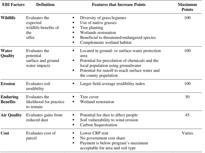
Figure 3.1 Wheat: Average Planted Acreage as a Proportion of State Total (1995-2005)... 14

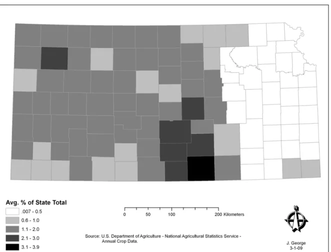
Figure 3.2 Sorghum: Average Planted Acreage as a Proportion of State Total (1995-2005) ... 15

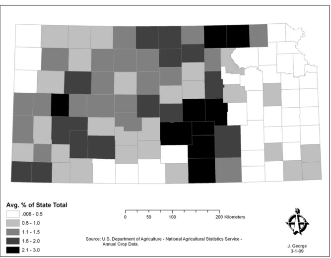
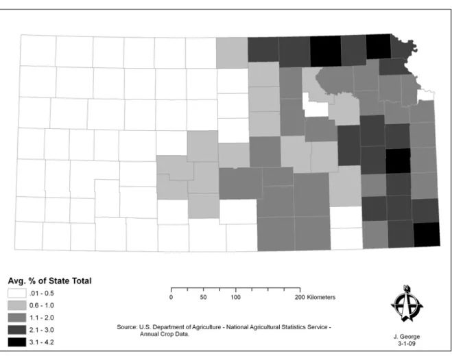
Figure 3.3 Corn: Average Planted Acreage as a Proportion of State Total (1995-2005) ... 16

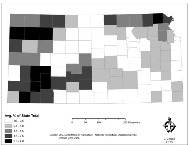
Figure 3.4 Soybeans: Average Planted Acreage as a Proportion of State Total (1995-2005)... 17

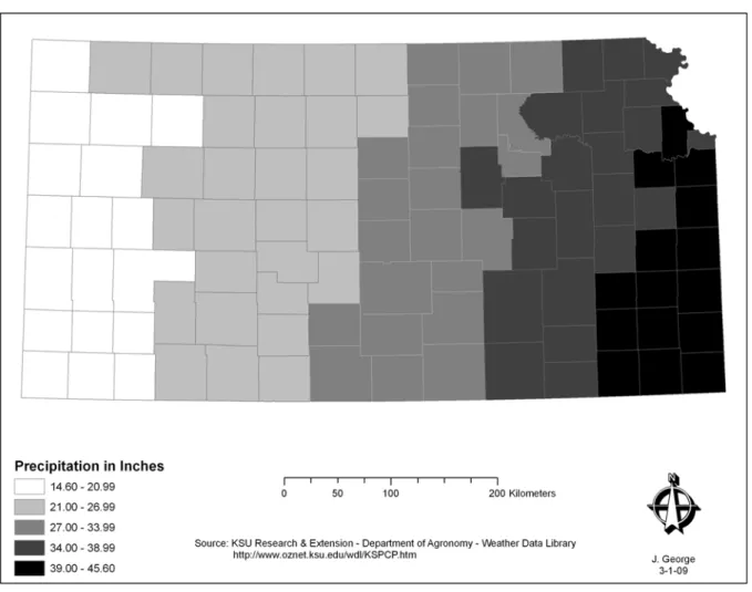
Figure 3.5 Precipitation: Normal County Annual Totals... 18

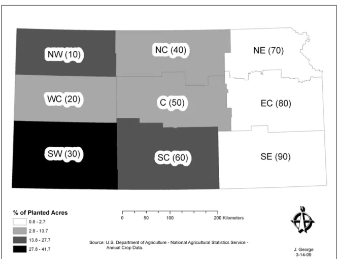
Figure 3.6 Agricultural Statistics Districts: Irrigated Cropland Average (1995-2005) ... 19

Figure 3.7 Total Annual CRP Enrollment in Kansas (1995-2005)... 20

Figure 5.1 Agricultural Census: Total Cropland in Production by District... 29

Figure 5.2 Wheat: Average Annual Prices Paid by District (1995-2005) ... 32

Figure 5.3 Sorghum: Average Annual Prices Paid by District (1995-2005) ... 32

Figure 5.4 Corn: Average Annual Prices Paid by District (1995-2005)... 33

Figure 5.5 Soybeans: Average Annual Prices Paid by District (1995-2005) ... 33

Figure 6.1 Average Annual Slippage for the Study Period (1995-2005) ... 36

Figure 6.2 Annual Slippage Rates by District (1995-2005) ... 37

Figure 6.3 Residual Plots for Regression Analysis... 39

Figure 6.4 Residual Plots for District Level Regression Analysis... 43

Figure B.1 Scatterplots: Output Prices vs. Slippage ... 92

Figure B.2 Scatterplots: Land Values vs. Slippage... 93

Figure B.3 Scatterplots: Wheat Input Costs vs. Slippage ... 93

Figure B.4 Scatterplots: Input Costs vs. Slippage... 94

Figure B.5 Scatterplots: Corn Input Costs vs. Slippage ... 94

Figure B.6 Scatterplots: Soybean Input Costs vs. Slippage... 95

(6)

List of Tables

Table 2.1 The Most Common & Highest Scoring Practices for CRP’s EBI (Classen et al. 2008) 8

Table 3.1 Top Five CRP Conservation Practices in Kansas (FSA 2003b) ... 22

Table 5.1 Regression Analysis Variables and Predicted Relationships... 34

Table 6.1 Initial Best Fit Regression Model Results ... 40

Table 6.2 District Level Regression Model Results. ... 44

Table 6.3 District Level Regression Model Results (grain crops average price and average costs variables removed)... 44

(7)

CHAPTER 1 - Introduction

Agricultural production in rural regions has long been a primary source of employment, driving rural economies, shaping their culture and values, and supporting urban populations. Government intervention in regard to agricultural production has also been a key force in rural areas. Although the catastrophe of the ‘Dust Bowl’ brought about the introduction of

government programs for soil conservation, the agricultural practices that had contributed to the problem not only continued, but intensified. After the Second World War, the developed world began to undergo a dramatic change in the form of productivist agriculture. As defined by Woods (2005), the central aim of productivist agriculture was to increase agricultural production, which happened through intensification, concentration, and specialization. The “productivist” shifts led to the increased use of large machinery and agri-chemicals, larger farm units, and a decrease in employment availability for the ‘generalist’ farm-worker (Troughton 2005). In other words, large, often corporate, farms began to replace the ‘traditional’ (smaller, more diversified, and more household-based) farms in rural regions, with production demands driven by a world market economy and government supports. Productivism’s central objective of increasing agricultural production was an unparalleled success, particularly through the changes that occurred in connection with what has become known as the Green Revolution, leading to an overabundance of agricultural goods that could not be sold at profit in the marketplace.

Governments intervened, in part by purchasing crop surpluses in an attempt to guarantee stable income to farmers. These price supports eventually began to place a financial burden on society as a whole, however. Farmers who had been encouraged to borrow money for the purchase of large machinery and on-farm improvements found themselves struggling to make ends meet due to increased interest rates and periods of drought leading to low crop production (Dudley 2000, Woods 2005). This ‘farm crisis’ resulted in moderate shifts in the way that the productivist agricultural model was applied, as many producers began to see the need for more stable and sustainable agricultural practices. As indicators of environmental degradation such as soil erosion and decreased water quality became increasingly evident, the developed world began to realize that sustainable agriculture was not a luxury, but rather a necessity (Rasmussen et al. 1998).

(8)

Throughout the development of conservation programs in the United States, there has been variation in both program goals and levels of success. Early efforts, such as the Soil Bank Program (SBP) started in 1956, focused on land retirement for the purpose of decreasing crop production in an attempt to increase commodity output prices, as well as diminishing erosion problems. With much of the focus on production and price control, the SBP was not very successful at decreasing environmental degradation (Potter 1998). In the early years (1986-1990) of the Conservation Reserve Program (CRP), there was also criticism that the program was too focused on land retirement for decreasing production, with a focus on maximizing the acreage enrolled rather than only retiring those lands that would have the greatest environmental benefits. The 1990 Farm Bill furthered the objectives of the CRP to include additional

environmental benefits, utilizing the Environmental Benefits Index (EBI) as a tool for targeting lands for retirement. Although a step in the right direction regarding the decrease of

environmental degradation on agricultural lands, economic drivers such as high commodity output prices and increased world market demand may serve to decrease conservation program efficiency and effectiveness.

Purpose

As geographers, we have the ability to perform spatial analysis at varying scales. The very nature of our work deals with identifying relationships. These are both skill sets that should prove invaluable in exploring the interconnected workings of human-environment interactions in rural areas. As noted by Woods (2005), environmental change in rural areas, including the degradation of the environment by modern agriculture and the encroachment of urban areas, is of growing interest to rural geographers concerned with land use issues. Geographers are well equipped to deal with the complexities of rurality, rural change, and rural governance (Cloke 1996).

This paper attempts to address concerns regarding a specific example of rural policy, namely the effectiveness of the CRP as a program for land retirement and those factors that alter program efficiency. Within the past decade there has been considerable geographical research pertaining to government agricultural policies such as the CRP and Conservation Reserve

(9)

et al. 2005), as well as more general considerations of the geographies of agricultural legislation (Dixon and Hapke 2003). In short, the discipline of geography is well established in the study of rural human-environment interactions and the associated policy decision making implications.

This study will further previous research (Leathers and Harrington 2000, Wu 2000) by applying the methods used for slippage calculation to the near-present – as close to the present as data availability allows – and attempting to identify those factors which contribute to change in CRP slippage.

Problem Statement and Objectives

The term “slippage” as it relates to the CRP occurs when producers plant newly

cultivated land or fallow acres, offsetting acreage that is retired through enrollment in the reserve program. Previous studies regarding slippage (Ericksen and Collins 1985, Leathers and

Harrington 2000, Wu 2000) indicated two major possibilities of factors contributing to slippage. The first factor is substitution and the second is output price increase. Slippage due to

substitution occurs when farmers with land enrolled in the CRP break previously uncultivated or fallow land in an attempt to make up the difference in cropped acreage. The Sodbuster and Swampbuster provisions were included in the Food Security Act of 1985 as an attempt to curb this practice, but enforcement problems have hampered their effectiveness (Wu 2000). Output price increase refers to the increase in slippage due to higher commodity output prices, and can result in farmers without enrolled land tilling previously uncropped areas. Higher output prices for agricultural commodities could be caused by the decrease in output (quantity supplied) associated with decreased production on CRP land or through increased market demand for agricultural outputs.

According to Wu (2000), if substitution is the major factor causing slippage, then preventing slippage could be accomplished by focusing on participating farmers. However, if output price increases are the major contributing factor, a focus on participant farmers would not be sufficient. Leathers and Harrington (2000) and Wu (2000) recognized the need for further temporal research regarding the magnitude of price related slippage. These studies also noted the negative impacts of government agricultural subsidies on conservation programs. As a follow-up, my research attempts to address the question: “Is there a relationship between

(10)

fluctuations in agricultural commodity output prices, input costs and Conservation Reserve Program slippage rates in Kansas?” The following tasks were accomplished to address this question:

1) Determination of the annual slippage rates for each county in Kansas between 1995 and 2005, using agricultural statistics at the county level.

2) Refinement of the study area by excluding those counties with a negative average annual slippage value for the study period (1995-2005).

3) Collection of annual grain crop output prices, input costs and land values in Kansas between 1995 and 2005, using agricultural statistics at the district and regional levels. 4) Completion of statistical analyses to determine the strength of relationships between

annual CRP slippage rates, agricultural commodity output prices and production costs.

Justification

The initial focus of the CRP was to reduce on-site soil erosion and excess crop

production, while positively affecting commodity prices. The goal was to establish conservation reserves totaling 40 to 45 million acres by the year 1990 (CES 1995). As of October 2008, Kansas had approximately 3.1 million acres of land enrolled in the CRP, bringing in $123.3 million in federal monies annually (FSA 2008). Considering the large amount of taxpayer funding spent on the program, any effort to better understand those factors that have a negative and/or positive impact on program benefits and efficiency is well justified and may aid further policy development.

Studies (Skold 1989, Riddel and Skold 1997) have indicated that cropland retirement policies such as the CRP have a minimal impact in terms of reduction in acreage of harvested cropland and even less effect on reducing production amounts. The latter may be due to an increase in per acre output or the fact that it is generally lower productivity land that is taken out of production, a side effect of retiring the most environmentally sensitive cropland that would be difficult to overcome. However inefficient the CRP may be in reducing excess crop production or increasing commodity prices, there are many studies (Cunningham 2005, Gray and Teels 2006, Lovell and Sullivan 2006) that extol the program benefits in terms of the decrease in

(11)

environmental degradation and increase in wildlife habitat. The purpose of this research is not to refute the site-specific environmental benefits of land retired through the CRP, but rather to determine those factors that decrease the overall efficiency of the program in achieving these benefits at a larger scale. Such information can help in future development and increased effectiveness of government conservation and land retirement programs.

Slippage calculations alone are a general indicator of the efficiency of the CRP in reducing the amount of land that is in crop production. These calculations do not take into account the unique benefits of individual parcels of land. However, placing previously

uncultivated or idle acreage into crop production (slippage) has a negative impact to some extent, no matter what the land’s EBI score (Gilley and Doran 1997). Therefore, identifying those factors that increase or decrease slippage rates can help to guide program decision making and increase the overall benefit to cost ratio of the CRP.

(12)

CHAPTER 2 - Background

Conservation Programs Development

The largest ‘payment for conservation’ programs can be divided into two groups based on their general approach. Land retirement programs remove land from production (generally cropland); working-land programs provide assistance to producers who maintain conservation practices on land in production. The following focuses on the development of land retirement programs.

Commodity price supports have been a mainstay in agricultural legislation since the farm depression of the 1920s and have included acreage reduction programs in some form since the Agricultural Adjustment Act (AAA) of 1933. Established as part of a New Deal agricultural policy, the focus of the AAA was the reduction of production by means of controlling crop acreages on individual farms (Hill 2003). Under the AAA, producers who complied with the approved reduction in crop acreage on their farm received a benefit payment. Issues regarding the funding source for the program led to the Supreme Court declaring the AAA unconstitutional in 1936. The Soil Conservation and Domestic Allotment Act of 1936 was passed as emergency legislation in response to this, shifting the focus of the overall program to income protection and resource conservation (Cochrane and Runge 1992). It is not surprising, given the timing of this legislation in relation to the ‘Dust Bowl’ era, that the resource conservation portion of this Act involved paying farmers to take acreage out of traditional row crop production and plant those acres to legumes and grasses.

Although agricultural legislation varied in terms of method, price supports in some form remained a constant throughout the 1940s. Levels of price support were minimally decreased in the early 1950s, but the combination of productivist agriculture leading to increased farm output and already mounting government grain stocks resulted in a large surplus (Bottum 1957). In an attempt to combat the growing surplus problem, the concept of the ‘soil bank’ was developed.

The Soil Bank Program (SBP), enacted in the Agricultural Act of 1956, consisted of two main parts. First, the Acreage Reduction Program (ARP) portion paid producers for enrolling acreage on which no crop would be harvested or cattle grazed. Between 1956 and 1958, approximately 21 million acres were ‘banked’ through the ARP (Cochrane and Runge 1992). The second part of the SBP was the first Conservation Reserve Program, which is often referred

(13)

to simply as the Soil Bank. This portion of the SBP paid producers for shifting below-average cropland into long-range conservation uses. Producers voluntarily enrolling in the three to ten-year land retirement program were required to maintain conservation cover on the land taken out of production, but producers were allowed to choose the sections of land that they enrolled in the Soil Bank under the SBP. Enrollment in the Soil Bank reached 28.6 million acres in 1960 with the last of the enrolled acres coming out of the program in 1972 (Cochrane and Runge 1992). The ARP was stopped in 1958 and contracts under the Soil Bank were not actively pursued after 1959. According to Cochrane and Runge (1992), the reasons for abandoning the two programs were the high cost of removing crop acres from production, the negative impact on rural areas from the provision that permitted whole farms to be taken out of production, and the lack of success in reducing total farm output.

A new version of the CRP was established by the Food Security Act of 1985 for the purpose of retiring environmentally sensitive cropland for a period of ten to fifteen years. The initial focus of the program was to reduce on-site soil erosion and excess crop production. Throughout the early years of the program (1985-1990), concerns were expressed regarding the maximization of acreage as opposed to the targeting of land based on benefit-to-cost ratios. In other words, the focus was on retiring as much land from production as possible rather than enrolling those properties that would result in the greatest environmental benefit from retirement. In response, the 1990 Farm Bill extended the objectives of the CRP to include on-farm and off-farm environmental benefits. The targeting mechanism introduced by the U.S. Department of Agriculture was the Environmental Benefits Index (EBI) (Yang et al. 2005). Surface water quality, groundwater quality, soil productivity, conservation compliance assistance, tree planting, acreage in critical watersheds, and acreage in conservation priority areas were equally weighted indicators of the EBI (Smith 2000). In addition to the utilization of the EBI, rental payments were restricted to an estimate for comparable cropland after adjusting for soil productivity (Yang et al. 2005). The EBI was redefined as part of the 2002 Farm Bill to include wildlife benefits, water quality benefits derived from reduced erosion, runoff and leaching, on-farm benefits of reduced erosion, enduring benefits, and air quality benefits from reduced wind erosion (FSA 2003a)(Table 2.1).

(14)

Table 2.1 The Most Common & Highest Scoring Practices for CRP’s EBI (Classen et al. 2008)

EBI Factors Definition Features that Increase Points Maximum Points Wildlife Evaluates the

expected

wildlife benefits of the

offer

Diversity of grass/legumes

Use of native grasses

Tree planting

Wetlands restoration

Beneficial to threatened/endangered species

Complements wetland habitat

100

Water Quality

Evaluates the potential

surface and ground water impacts

Located in ground- or surface-water protection area

Potential for percolation of chemicals and the local population using groundwater

Potential for runoff to reach surface water and the county population

100

Erosion Evaluates soil erodibility

Larger field-average erodibility index 100

Enduring Benefits

Evaluates the

likelihood for practice to remain

Tree cover

Wetland restoration

50

Air Quality Evaluates gains from reduced dust

Potential for dust to affect people

Soil vulnerability to wind erosion

Carbon Sequestration

45

Cost Evaluates cost of parcel

Lower CRP rent

No government cost share

Payment is below program’s maximum acceptable for area and soil type

Varies

According to Yang et al. (2005), research assessing the CRP indicated that the shift to the EBI was helpful in increasing the cost effectiveness of the program. However, alternate studies (Leathers and Harrington 2000, Wu 2000) analyzing slippage were not as optimistic regarding the effectiveness of the CRP, especially regarding the decrease of soil erosion.

Slippage

The phenomenon of “slippage,” as it relates to agricultural acreage reduction programs, can be traced back to early appraisals of the AAA in the 1930s. As noted by Cochrane and Runge (1992), agricultural producers in the 1930s found ways around the crop-specific

(15)

crops on the acreage which resulted in little to no actual reduction in production. Although acreage reduction programs have changed significantly since the AAA, the concept of slippage remains a useful tool for estimating program effectiveness.

There are two main types of slippage that can be analyzed when considering land retirement programs: acreage slippage and yield slippage. Acreage slippage compares the total amount of acreage removed from production under the retirement program to the amount of land in production post-retirement and can be calculated in terms of total acreage in production or for specific crops. Yield slippage refers to the quantity of commodities produced post-retirement of program lands in comparison to quantities prior to program enrollment. Because the main intent of the AAA programs during the 1930s was to reduce production through the control of crop acreages, yield slippage was a good indicator of program effectiveness (Cochrane and Runge 1992). However, given the multiple-objectives of the current CRP, acreage slippage allows for a more holistic analysis of overall program success and is the focus of this paper.

The occurrence of acreage slippage takes place when agricultural producers plant either newly cultivated land or previously fallow fields, offsetting the acreage retired under the program. These producers may or may not be participants in the CRP: acreage slippage may occur either with substitution (of uncropped area for the acreage enrolled in a retirement

program) or with non-enrolled farmers who expand their cultivated land (perhaps in response to an increase in output prices). In the case of those who have land enrolled in the CRP, money saved on input costs by not cultivating the retired land combined with the CRP rental payment may afford them the ability to cultivate previously idle, less productive land. In this case, so long as the property had been previously cultivated and a conservation plan developed, Farm Bill provisions provide no means of penalty for these actions. Producers without land enrolled in the CRP may begin to cultivate new ground or less productive fields in anticipation of higher

commodity output prices that may result from a reduction in area production due to land retirement. Producers involved in other government programs, such as crop insurance or farm loans, they still required to have a conservation plan in place if the land is considered highly erodible. They also are forbidden from plowing up previously uncultivated grasslands under the Conservation Compliance and Sodbuster provisions of the 1985 Farm Bill. However, those producers not involved in government programs are able to cultivate any and all land under their

(16)

control because the penalties associated with Farm Bill provisions are limited to the denial of access to all federal agriculture assistance programs.

Ideally, the number of acres in production would be directly reduced by the number of acres retired under the CRP. In reality, acreage reduction programs generally only reduce total crop acreage by a percentage of that which is removed from production by program enrollment (Ericksen and Collins 1985). The resulting offset due to increased plantings on unrestricted acres is slippage and is measured as a factor from zero to one. A slippage factor of zero indicates that for every acre removed from production, total acreage in production is reduced by one acre. In other words, program retirements have been completely effective. Likewise, a slippage factor of one means that total production was not at all reduced by the program acreage being removed from production.

Economic Impacts of CRP

The concept of equity among producers enrolling land in the CRP has been a major issue. The broad problem arose from a uniform bid cap within a region where individual parcel

productivity may greatly differ. The results were a greater burden on those producers with highly productive land who wished to enroll a portion of their land in the CRP than those enrolling less productive land in the program (Young et al. 1991). Revisions in the 2002 Farm Bill addressed these concerns by setting bid maximums based on county-level average cropland rental rates and adjusting these rates for field-specific productivity.

Although there is a 25 percent cap on the amount of land that can be enrolled in the CRP within each county, the impact on the local economy from taking this land out of agricultural production is still an issue of concern. As noted by Martin et al. (1988), “while individual farmers may benefit from participation, there may be [a] net adverse impact on the community if the retired land is relatively productive or if the inputs that are no longer purchased would have been purchased locally”. The negative impacts on the local economy can be further compounded if the monetary CRP benefits are going to a landowner who no longer resides in the area (Martin et al. 1988). Revisions within the 2008 Farm Bill address this issue by giving preference to locally-residing producers over absentee landowners for program enrollment, all other criteria being equal. In rural areas where the CRP reaches the 25 percent per county enrollment level,

(17)

the local decrease in demand for farm inputs can have a major impact. Couple this with commonly occurring depopulation of these areas, and it is even more challenging for local suppliers to stay in business.

Enrollment in the CRP does affect the supply of agricultural commodities, making it a useful tool for the reduction of excess crop production (Taff 1990). However, this would only hold true for those counties where any reduction in crop production is not offset by slippage. In turn, the decrease in commodity supply may increase commodity prices, adjusting the

relationship between potential production income from the land and income gained through enrollment in the CRP. This can lead to increased slippage in regard to the program and decreased re-enrollment upon completion of program contracts.

As previously mentioned, the CRP was criticized early on for attempting to maximize acreage enrolled in the program. Although Congress mandated that the CRP be run as an auction with the hopes that this would provide incentive for landowners to submit bid prices that

reflected the land’s true rental values, difficulties with the initial implementation of the program (1985-1990) transformed it into an “offer system” where anyone with eligible land could enroll and be paid at the bid cap price (Smith 1995). This raised some questions regarding the size of the CRP relative to the amount that was being spent on the program. Essentially, what critics were saying is that with this method, the costs of the program outweighed the benefits (marginal cost was higher than marginal benefit). In an attempt to decrease marginal cost relative to marginal benefit, rather than decrease the size of the program, determination of land eligibility for enrollment in the CRP was based on the Environmental Benefits Index and program payments were based on an estimate of production capability on the enrolled lands.

Land enrolled in the CRP is privately owned; however, with enrollment in the program comes certain rules and regulations regarding the use of not only the land enrolled, but also all other land owned by the agricultural producer. The Sodbuster, Swampbuster, and Conservation Compliance provisions included in the Food Security Act of 1985 require that no previously uncultivated ground is put into production and that all land in production meets appropriate conservation practices. Failure to comply with these provisions can result in the loss of

eligibility for certain farm program benefits if it is determined that the producer was not acting in ‘good faith’. This would seem to be a large enough penalty to deter violation of the rules. However, confirmation of compliance with these provisions has proven difficult, given the vast

(18)

spatial extent of CRP lands (Wu 2000). Increasing agricultural commodity prices also provide economic incentive for the violation of these provisions.

Assuming that slippage does not surpass the benefits of the program, agricultural land retirement through the CRP reduces the external costs of farming. These externalities occur where producers do not incur the full cost of their actions. Examples of externalities associated with agricultural production include soil erosion and fertilizer runoff which pollute both surface water and groundwater, emissions from the use of fossil fuels for production purposes, the release of carbon from tilling the soil which leads to air pollution, and in certain areas substantial depletion of groundwater supply through irrigation. Removing land from production effectively reduces these externalities.

Because producer decisions to enroll in the CRP may cause the price of agricultural commodities to increase, due to a decrease in production and available quantities, it can also be said that the program has an external economy for other producers. External benefits may exist in the form of decreased pollution for those downstream from land enrolled in the CRP. Again, as long as the environmental benefits gained from those lands enrolled in the CRP are not offset by slippage, the improved water quality could be considered an external benefit for those downstream from the property.

With increasing prices of agricultural commodities and many CRP contracts set to expire, a major issue with current CRP policy is that of rental rates and the extension of CRP land contracts. A study (Cooper and Osborn 1998) conducted around the time of the last large

contract expiration found that, given the then-current averages for CRP rental payments, only 50 percent of enrolled landowners would be likely to extend their contracts. Given such indications, it will be interesting to see what impact recent commodity prices will have on landowner

decisions to re-enroll in the CRP. The ability to profit additionally from the harvest of biomass for biofuel production on CRP land and permitted haying or grazing (with payment reductions as outlined in the 2008 Farm Bill) may play a crucial role in these decisions.

(19)

CHAPTER 3 - Study Area

According to the Kansas Energy Plan (2007), approximately 94 percent (49.2 million acres) of Kansas land is used for agricultural production and wildlife habitat. As calculated from crop statistics reported by the National Agricultural Statistics Service (NASS), row crop

production accounts for approximately 20.8 million of these acres (1995-2005 average). In comparison to this, the 3.1 million acres of land currently enrolled in the CRP within the state seems rather minuscule. However, as the largest cropland retirement program to date, those acres retired under the CRP are a crucial part of ongoing attempts to decrease the environmental degradation that results from agricultural production on marginally suitable lands. Kansas has the third highest total acreage enrolled in the CRP, slightly trailing Montana (3.2 million acres) and Texas (3.8 million acres) (FSA 2009). Although it may rank third in total acreage, when enrolled acreage is considered with respect to total land area among these three states, Kansas comes out on top with approximately 5.9 percent of total land area enrolled in the CRP (Montana 3.4 percent; Texas 2.3 percent).

The state of Kansas represents an area with a high degree of spatial variability in crop production, and methods of production, due to a spatially disparate precipitation pattern, regional differences in access to and need for irrigation, and heavily weighted population centers within the eastern third of the state that results in differing land ownership patterns. Given the state’s emphasis on agricultural production, the regional variability in production, and the large acreage enrolled in the CRP, Kansas lends itself well to the analysis of CRP slippage and the

determinants thereof.

Agriculture in Kansas

There are four main crops under production within the state of Kansas: wheat, sorghum, corn, and soybeans. Wheat accounts for approximately 50.25 percent of total row crop planting within the state (percentages based on total planted acreage averages from 1995-2005).

Regionally, wheat is fairly evenly dispersed throughout the western two-thirds of the state, with some notable concentrations in the south-central area (Figure 3.1). Sorghum is the second most common crop, representing approximately 17.2 percent of total row crop planting. As with wheat, sorghum is common throughout Kansas, but is more concentrated in the south-central,

(20)

north-central and southwestern portions of the state (Figure 3.2). Corn is slightly less common than sorghum, at 14.5 percent of total crop acreage. Corn is also less spatially dispersed than wheat and sorghum, with large concentrations of planted corn in the southwestern and northwestern areas and some minor concentration in the extreme northeast (Figure 3.3). Soybeans are approximately 12.5 percent of total planted row crops. As seen in Figure 3.4, soybeans are primarily grown in the eastern one-third of the state, an area with lower numbers of the top three grain crops in comparison to the rest of the state. This is due primarily to

calcareous soils in the central and western portions of the state and the common resulting problem of iron chlorosis in soybeans (AESCES 1997). Alternative crops such as sunflowers, upland cotton, and dry edible beans make-up the remaining 5.5 percent of total crops.

(21)

(22)

(23)

Figure 3.4 Soybeans: Average Planted Acreage as a Proportion of State Total (1995-2005)

Annual precipitation varies across the state, decreasing in an east-to-west gradient (Figure 3.5). Not surprisingly, the use of irrigation reflects the lack of rainfall in the western two-thirds of the state and is compounded in the southwestern region by the concentrated planting of corn, a crop with a high requisite for water (Figure 3.6). The primary source of water for irrigation in this High Plains area is the vast Ogallala Aquifer. The availability of affordable technology to tap this resource after World War II (Kromm and White 1992) changed this portion of the state from a drought stricken area of low production to one of the most agriculturally productive areas in the state (Peterson et al. 2003). Unfortunately, the high use and slow recharge of aquifer waters has led to dramatic decreases in the level of the water table and there are now areas where it is no longer economically feasible to access the water for irrigating crops.

(24)

(25)

Figure 3.6 Agricultural Statistics Districts: Irrigated Cropland Average (1995-2005)

Population densities in eastern Kansas are much higher than the rest of the state. Historically, large settlements within the state were located along the Kansas River, its

tributaries, and the Arkansas River (Self and White 1986). The combination of a high population density and less open terrain has resulted in smaller farm units in the eastern third of the state. In comparison, the wide-open expanses of the high plains region in the west has lent itself well to the development of very large, often corporate, farms.

Conservation Reserve Program in Kansas

Total enrollment in the CRP varied throughout the study period (1995-2005), with lows of approximately 2.5 million in 1999 and 2000 (Figure 3.7). Of the 3.1 million acres in Kansas that are currently enrolled in the CRP, approximately 2.6 million acres are located in the western two-thirds of the state (Figure 3.8). Interestingly, despite the large spatial difference in

(26)

contracted acreage, the number of CRP contracts is fairly evenly distributed throughout the state. The reason for the spatially disparate CRP acreage is a combination of land ownership patterns, terrain, soil types, and the conservation practices that are most widely used in different regions of the state. Many CRP practices in the eastern portion of the state enroll buffers and filter strips rather than the large expanses of grassland that are seen in central and western Kansas.

Figure 3.7 Total Annual CRP Enrollment in Kansas (1995-2005)

2300000 2400000 2500000 2600000 2700000 2800000 2900000 3000000 1995 1996 1997 1998 1999 2000 2001 2002 2003 2004 2005 Year C R P E n ro ll m e n t (acr es)

(27)

Figure 3.8 CRP Distribution in Kansas (March 2009)

Currently, within the CRP there are 38 Conservation Practices (CP), ranging from the planting of native grasses to the construction of erosion control structures along stream banks. This total excludes further breakdowns within each practice such as Tree Planting (CP3) and Hardwood Tree Planting (CP3A). The most common Conservation Practices in Kansas (Table 3.1) are Vegetative Cover–Grass–Already Established (CP10), Establishment of Permanent Native Grasses (CP2), Restoration and Management of Declining Habitat (CP25), Filter Strips (CP21), and Habitat Buffers for Upland Wildlife (CP33). Combined, these account for

approximately 97.8 percent of all acres enrolled in the state.

The difference in land ownership patterns and Conservation Practices between the eastern one-third and western two-one-thirds of the state is evident when the contract data are broken down. While CP10 is the most common practice in both regions, it makes up only 25 percent of total

(28)

contracts in the east and nearly 40 percent of contracts in the west. The average tract size of the CP10 contracts also differs regionally, with an average of 18.9 acres in the east and 56.5 acres in the west. Another major difference is the use of filter strips (CP21). In the eastern one-third of the state, CP21 is the second most common practice, accounting for nearly 25 percent of

contracts and averaging only 2.4 acres per tract. In the central and western portions of the state, CP21 totals only 3 percent of all contracts.

Table 3.1 Top Five CRP Conservation Practices in Kansas (FSA 2003b) Conservation

Practice (CP)

Practice Purpose Percent of Total

Acres Enrolled 10 Vegetative Cover –

Grass – Already Established

Reduce soil erosion & sedimentation

Improve water quality

Enhance wildlife habitat

52.3

2 Establishment of Permanent Native Grasses

Restore a plant community similar to its historic climax or the desired plant community

Provide or improve forages for livestock

Provide or improve forage, browse or cover for wildlife

Reduce erosion by wind and/or water

Improve water quality & quantity

27.6

25 Restoration & Management of Declining Habitat

Restore land or aquatic habitats degraded by human activity

Provide habitat for rare & declining wildlife species by restoring & conserving native plant communities

Increase native plant community diversity

Manage unique or declining native habitats

15.9

21 Filter Strips Reduce sediment, particulate organics, and sediment adsorbed contaminate loadings in runoff & surface irrigation tailwater

Reduce dissolved contaminate loadings in runoff

Restore, create or enhance herbaceous habitat for wildlife & beneficial insects

Maintain or enhance watershed functions & values

1.0

33 Habitat Buffers for Upland Wildlife

Create corridors for wildlife movement

Provide wildlife food

Provide nesting, brood & winter cover

Provide habitat for beneficial insects

Reduce erosion & improve water quality

1.0

(29)

CHAPTER 4 - Literature Review

In an attempt to gain a more holistic view of the recent research pertaining to the CRP, my literature review ranges outside the scope of those studies specific to the topic of CRP

slippage. As a multiple objective program, it is important to include this research to gain a better understanding of how alternate studies view the benefits of the CRP.

Slippage

Early research regarding the phenomenon of slippage as it related to acreage reduction programs included that of Ericksen and Collins (1985). While this research pertained to programs predating the current CRP, the premise and methods utilized for calculating slippage rates are similar. The major difference is in the goals of the acreage reduction programs. The CRP was the first acreage reduction program to place much importance on the reduction of soil erosion. Prior to the CRP, the major focus of acreage reduction programs was to control crop production and increase agricultural commodity prices. Ericksen and Collins (1985) analyzed the effectiveness of acreage reduction programs at actually reducing total crop supply. By comparing the annual change in harvested acreage with the change in acreage idled through reduction programs in the United States, they were able to calculate annual slippage rates. Their results led them to conclude that these early acreage reduction programs were inefficient at reducing crop supplies because of increased plantings on unrestricted acres and a reduction in the impact from idling lower yielding lands.

Previous research regarding slippage in the CRP has varied in both the spatial extent of the study area and the approach or methods used for the analysis. Leathers and Harrington (2000) focused specifically on the issue of land slippage in the 14-county area of Southwestern Kansas from 1988 to 1994. Because acreage was also enrolled in both the Acreage Conservation Reserve (ACR) and the Conservation Use for Pay program (CUPAY) during the study period, the annual conservation acreage totals included those acreages and that of the CRP. Using agricultural statistics, slippage rates were calculated at the county level for each year in the study period and remotely sensed data was analyzed for a refined study area. Slippage rates varied from one county to the next, with some counties showing more year to year variability. Overall

(30)

results indicated that slippage in Southwestern Kansas greatly reduced the effectiveness of the CRP at decreasing soil erosion.

A similar study conducted by Wu (2000), analyzed the slippage effect on a much larger 12 state region in the central U.S. The study outlined the ways in which both substitution and output price increase can bring fallow or unbroken land into production. Data for the slippage analysis were acquired from the 1982 and 1992 National Resource Inventories produced by the Natural Resource Conservation Service (NRCS) and county-level CRP summary data from the Economic Research Service (ERS). A multivariate regression model was used to examine the impact of the CRP on the acreage of non-cropland converted to cropland. The dependant variable was acreage of non-cropland converted to cropland between 1982 and 1992 as a proportion of the total land area in each agricultural statistical unit. Independent variables included acres of cropland enrolled in CRP by 1992 and other characteristics, such as farm size and population. The variables included in the regression explained 45 percent of the variation in the converted cropland acreage according to the analysis. The study concluded that substantial slippage effects were present in the CRP and, more specifically, that for each 100 acres of land retired under the CRP in the central U.S., 20 acres of non-cropland were converted to cropland.

Soil Quality and Erosion

The National Research Council’s (1993) analysis of agricultural impacts on soil and water quality stated that “protecting soil quality, like protecting air and water quality should be a fundamental goal of national policy” (p. 18). Soil quality not only affects the productivity of the land, but is also connected to the physical condition of other resources including air, water, plants, and animals (Mausbach 1996). According to a study conducted by Pimental et al. (1995), approximately 90 percent of cropland in the U.S. is losing soil at what is considered to be above a sustainable rate.

Realizing that CRP contracts are not all continuously enrolled, a study by Gilley and Doran (1997) in Northern Mississippi attempted to determine the post-enrollment soil erosion potential of CRP land once it was returned to cropland. Soil erosion rates were known for the test field prior to enrollment and were compared to erosion rates after the one-time CRP field had been tilled and left fallow for nine months. The results indicated that soil erosion rates prior to

(31)

enrollment in the CRP were very similar to erosion rates after the conservation cover had been tilled.

Baer et al. (2000) constructed a study to determine the impacts of the CRP on soil quality in terms of carbon and nitrogen content. They examined the soil quality from samples obtained at a depth of 2 to 4 inches from fields recently converted from agricultural production to native perennial grasses through the CRP, fields that had been in the CRP for a period of ten years, and fields of native prairie. While both of the CRP samples were lower in terms of total carbon and nitrogen pools in comparison to the native prairie, the long-term (ten year) samples did show significant increases. Based on the results and comparisons of the analyzed soil samples, the authors concluded that the CRP does promote soil restoration; however ten years is not a sufficient timeframe for restoring soils to pre-cultivation quality levels.

Water Quality

Khanna et al. (2003) indicated that the growing concern over the negative impacts of agricultural activities on water quality has changed the focus of land retirement programs from reducing on-site soil erosion to reducing damages to water bodies caused by sediment and chemical runoff. This shift in priorities is indicated by the introduction of the Conservation Reserve Enhancement Program (CREP) as a modification to the CRP. This study attempted to identify areas in Illinois where implementation of the CREP would be most effective at meeting the state’s environmental goals regarding the reduction of sediment and nutrient loadings. The study used an integrated framework to combine both spatial and biophysical attributes of land within the sample watershed with a hydrological and an economic model. Not surprisingly, the results indicated that croplands that are highly sloping and adjacent to water bodies should be selected for retirement. The more interesting portion of the results resulted from the inclusion of the economic model, which indicated that a marginal value rental payment scheme would

achieve the program goals at a lower cost than a productivity-based rental scheme.

Lovell and Sullivan (2006) analyzed the effects of conservation buffers and then looked at the relationship between buffers and the CRP. It is noted that conservation buffers are extremely positive for the ecological health of rural landscapes, decreasing soil erosion and increasing water quality. Water quality benefits associated with buffers include reduced

(32)

sediment loading from runoff and decreased leaching of agricultural chemicals and fertilizers. Because of the perceived value of buffers, the authors note, the U.S. Department of Agriculture is committed to increasing buffer adoption through the CRP, which is the primary program for funding buffers in the U.S. However, U.S. policy makers have not fully embraced the idea of conservation buffers. Recommendations that resulted from this study included modifying policies to better reflect the preferences of landowners and society, a multi-disciplinary study of buffer systems at the watershed scale, and designing buffers that consider aesthetic preferences and for varying locations.

Wildlife Benefits

Due to the fact that approximately 70 percent of land in the lower 48 states of the U.S. is in private ownership, land retirement programs are very important to the conservation of fish and wildlife (Burger 2006, Gray and Teels 2006). Although soil conservation was the original focus of CRP contracts, the perennial vegetation planted also provided habitat for wildlife (Gray and Teels 2006). The increased environmental emphasis of CRP enrollment requirements, as indicated by the switch to the EBI, reflects the importance of reserve programs on wildlife habitat, and so do the many studies that document the benefits of habitat improvement. These studies range from specific impacts of reserve lands on a single species, to overall effects of conservation lands on biodiversity.

Fields et al. (2006) studied the impact of CRP lands on the nesting and brood survival of the lesser prairie-chicken in west-central Kansas. The study determined that the probability of nest survival was best determined by the age of the nest and brood, timing during the season, age of the brooding female, and precipitation during the brooding period. Although location of nests and broods were considered, the fact that some nesting/brooding sites were located on CRP lands was not determined to be a significant factor in determining survival rates. In other words, there appeared to be no benefit to those nesting/brooding sites that were located on CRP lands during this study period.

A study by Kamler et al. (2004) compared the home ranges and seasonal habitat of coyotes in northwestern Texas on native prairie, farmland, and CRP land, in an attempt to determine impacts of CRP on populations and ranges. The study indicated that CRP fields do

(33)

provide important cover for coyotes, however the authors emphasize that CRP lands were the only tall permanent vegetation in their study area. Coyotes were divided into two distinct groups, residents and transients, and the impacts of the different cover types were measured for either group. The research showed the importance of CRP habitat as areas for resident coyote dens and foraging habitat for transients. The methodological approach for this study did not allow for the measurement of possible carrying capacity increases on CRP lands; however, the authors noted the likelihood of an increased capacity based on the high use of CRP areas by both groups of coyotes.

A study conducted by Cunningham (2005), attempted to compare the relative benefit for grassland songbirds of public grasslands maintained as habitat in the Midwestern U.S. with private land that was retired in the CRP. Her study area was in southern Minnesota, where bird survey data from CRP fields and public lands were gathered. She then ran an assessment of fragmentation utilizing GIS. Results indicated that native songbird abundance and diversity were greater on CRP lands. The cause of this appears to be the vegetation composition, with more dense grasslands on CRP lands than on public lands. The author attributes this to funding differences, and notes that temporal variation of CRP lands could have a strong influence on the success or failure of biodiversity conservation in this region.

Klute, Robel, and Kemp (1997) addressed the issue of non-reenrollment of CRP lands and the associated impact on grassland birds in Kansas. The timing of this study was based on the fact that unless renewed, many CRP contracts were set to expire in 1997. The study

indicated that up to 70 percent of land in Kansas that was not re-enrolled would be converted to pasture. The study therefore compared the avian use of CRP areas with that of pastures in order to determine if the conversion of CRP to pasture would negatively impact grassland birds. The authors found that CRP lands in the study area had less dense vegetation than pastureland during portions of the year, although vegetation on CRP lands was taller late in the summer. Total avian abundance was greater in pastures than in CRP fields. As such, it was concluded that the conversion from CRP to pasture in Kansas would not be detrimental to grassland bird

populations if the land were moderately grazed.

(34)

CHAPTER 5 - Methods

Because crop reports are made annually at the county level, my analysis was conducted based on these spatial units, rather than ecological units such as watersheds. The slippage calculations are based partly on the county crop figures as made available through the USDA National Agricultural Statistics Service (NASS). Through this source, annual acreage totals for both planted and harvested crops were compiled for all 105 counties in Kansas. A state level branch of the NASS, the Kansas Agricultural Statistics Service (KASS), provided the source for historical reports regarding average annual prices paid for the four main grain crops (wheat, sorghum, corn, and soybeans) and average annual land values for irrigated, dry-land, and

pastureland. Finally, regional annual production costs were obtained from the USDA Economic Research Service (ERS) for each of the four main grain crops. These production costs include average annual prices (in dollars) paid for seed, fertilizer, custom operations, and energy inputs per planted acre for each crop.

The study period of 1995-2005 was chosen for several reasons. First, during this timeframe the CRP accounted for the overwhelming majority of land in retirement programs within the state of Kansas. Second, restrictions in data availability for one or more of the independent variables limited the length to this eleven year period. Finally, the period of 1995-2005 contains significant variations in regard to output prices paid and input costs for

agricultural commodities.

Slippage Calculations

The method used for slippage calculations is the same as that which was employed by Leathers and Harrington (2000) when analyzing the effectiveness of the CRP in reducing soil erosion in a 14 county area of southwestern Kansas. Calculations are based on county level agricultural statistics and land retirement program enrollment numbers using the following equation:

S = {1.0 – [(A – A*) / L]} x 100,

where S is the slippage factor, A is the acreage that would be in production without CRP, A* is the actual acreage of crops, and L is the acreage enrolled in the CRP.

(35)

In determining the acreage that would be in production without the CRP (A), several factors must be considered. Leathers and Harrington (2000) used the average number of acres harvested in 1980, 1981, and 1982, rather than the three year period immediately prior to the CRP, because there was no land retired through alternate acreage diversion programs in 1980 and 1981 and very few acres retired in 1982. For this same reason, I have chosen to use this time period in determining the county level base acreage for slippage calculations in my study. Using this time period does introduce a potential source of error. If the total acreage in production was increasing post-1982, then the base acreage (A) would be too low causing inflation in the

calculated slippage rates. An analysis of district level total cropland figures, gathered from the USDA NASS Census of Agriculture (1982, 1987, 1992, 1997, 2002), shows the total acreage for 1982 as equal to or higher than the total acreage for 1997 and 2002 for all districts (Figure 5.1; see also Figure 3.6). This lower total cropland acreage cannot be attributed to the introduction of the CRP as the Census of Agriculture includes reserve program lands as idled cropland in

determining this figure. Therefore, using the average acreage in production from 1980-1982 as the base acreage for each county should not produce any significant inflation in the slippage calculations.

Figure 5.1 Agricultural Census: Total Cropland in Production by District

0.00 1.00 2.00 3.00 4.00 5.00 6.00 Dist. 10 (NW) Dist. 20 (WC) Dist. 30 (SW) Dist. 40 (NC) Dist. 50 (C) Dist. 60 (SC) Dist. 70 (NE) Dist. 80 (EC) Dist. 90 (SE) M il li ons of A c re s 1982 1987 1992 1997 2002

(36)

An additional possible source of error worth noting is the agricultural practice of double-cropping. Double-cropping occurs when two different crops are grown on the same acreage during a growing season. Unfortunately, acreage figures for this practice are not available at any scale for the state of Kansas. Because of the lack of available data, a method must be developed in an attempt to overcome the possibility of overestimating acreage in production due to this practice. Leathers and Harrington (2000) used the total acreage harvested rather than the total acreage planted in an attempt to remove the impact of double-cropping on reported acreage in production. I have found that the impact of poor harvest years introduces a significant amount of undue variation on slippage calculations. To decrease the impact of poor crop years I calculated a 25 year (1980-2004) average of the proportion of planted crops that were harvested for each county. The total reported planted acreage for each county was then multiplied by the 25 year average percentage harvested for each year in the study (1980-1982 and 1995-2005); the results were used for both the acreage in production without CRP (A) and the actual acreage of crops (A*), effectively removing the influence of extremely poor harvest years while still accounting for the practice of double-cropping. While this method may help to curb the inflation of slippage calculations created by overestimation of actual acreage in production, some inflation may still exist.

As traditional crop rotation methods have given way to continuous cropping practices fueled by the increased use of fertilizers, overestimation of actual acreage in production is a difficult obstacle to overcome without the availability of more detailed data regarding the

practices taking place on the reported acreage. Another area where the lack of detailed data may impact the accuracy of total acreage in production estimations is the scale at which individual crops are reported on annually. Due to privacy concerns, NASS often combines counties when reporting totals for alternative crops within Kansas such as oats, rye, and barley. Because of this, it is impossible to gather county level data for all crops that are planted within each county on an annual basis. However, these alternative crops together only account for an average of

approximately 5.5 percent of statewide total planted crops within the study period (1995-2005). The lack of these crops in all figures for total actual planted acres (A*) annually should not significantly impact the accuracy of slippage calculations and may help to mitigate any overestimation of actual planted acreage.

(37)

Figures for Ford County can be used as an example of how the slippage rates are calculated: in 1980-1982, after adjusting for the 25 year (1980-2004) average proportion of planted crop acreage that was harvested (89.91 percent), an average of 317,534 acres were in production. In 1995, after making the adjustment (average harvesting of 89.91 percent of planted acreage), 314,327 acres were under cultivation and 49,318 acres were enrolled in the CRP. Slippage for 1995 equaled: 1 - [(317,534 - 314,327)/49,318], or 0.935. In other words, for every 100 acres enrolled in the CRP, only 6.5 acres were taken out of production; the remaining 93.5 percent were slipped acres.

Agricultural Commodity Pricing & Costs

Due to the lack of available county level data regarding annual prices paid for agricultural commodities, these data had to be gathered at the district level. NASS and KASS divide the state of Kansas into nine statistical district that each include anywhere from eight to fourteen counties. The divisions are labeled as Northwest, West-Central, Southwest, North-Central, Central, South-Central, Northeast, East-Central, and Southeast. The data sets that were collected from the district level KASS historical reports include the average annual price paid per bushel for wheat, sorghum, corn, and soybeans, and the average annual land values for irrigated cropland, non-irrigated cropland, and pastureland. Variations in annual average prices paid for the four main grain crops were very slight among districts through the study period (Figures 5.2, 5.3, 5.4, 5.5), with highs and lows generally occurring in the same years for all crops. Because of the district-level similarities among reported prices paid, any spatial relationships that may exist between CRP acreage slippage and agricultural commodity output prices are not easily observed. Given the high degree of spatial variability for the average CRP slippage rates, further analysis regarding annual variation in output prices and slippage rates within each district (rather than across districts) may be beneficial.

(38)

Figure 5.2 Wheat: Average Annual Prices Paid by District (1995-2005) 0.00 1.00 2.00 3.00 4.00 5.00 6.00 1995 1996 1997 1998 1999 2000 2001 2002 2003 2004 2005 Year P ri ce P ai d / B u sh el ( $) NW WC SW NC C SC NE EC SE

Figure 5.3 Sorghum: Average Annual Prices Paid by District (1995-2005)

0.00 1.00 2.00 3.00 4.00 5.00 6.00 7.00 1995 1996 1997 1998 1999 2000 2001 2002 2003 2004 2005 Year P ri ce P ai d / B u sh el ( $) NW WC SW NC C SC NE EC SE

(39)

Figure 5.4 Corn: Average Annual Prices Paid by District (1995-2005) 0.00 0.50 1.00 1.50 2.00 2.50 3.00 3.50 4.00 4.50 1995 1996 1997 1998 1999 2000 2001 2002 2003 2004 2005 Year Pr ic e Pa id / B u s h e l ( $ ) NW WC SW NC C SC NE EC SE

Figure 5.5 Soybeans: Average Annual Prices Paid by District (1995-2005)

0.00 1.00 2.00 3.00 4.00 5.00 6.00 7.00 8.00 1995 1996 1997 1998 1999 2000 2001 2002 2003 2004 2005 Year Pr ic e Pa id / B u s h e l ($ ) NW WC SW NC C SC NE EC SE

Because no data are available at the county, district, or state level, I was forced to include agricultural input costs based on data from a larger area. The USDA ERS produces historical reports on commodity costs and returns at the regional level. While this is not ideal, the data should be sufficient given the lack of intrastate variation in average input costs. However, comparing regional scale data to county level CRP slippage rates may be troublesome for

(40)

statistical analysis, introducing a high degree of correlation between predictor variables. The region used is termed the Prairie Gateway by the ERS, and includes all of Kansas, southern Nebraska, eastern Colorado and New Mexico, western Oklahoma, and all of Central Texas. The data collected from these reports includes the average cost per planted acre for wheat, sorghum, corn, and soybeans, including costs for seed, fertilizer, custom operations (planting and

harvesting), and energy inputs (fuel, lube, and electricity). This annually compiled data set uses a sampling method from which estimates of the regional averages are derived.

Statistical Analysis

Using the annual slippage calculations as my response variable, a multivariate linear step-wise regression analysis was used to examine the relationships between CRP slippage and agricultural commodity output prices and input costs (Table 5.1). The software utilized in Table 5.1 Regression Analysis Variables and Predicted Relationships

Response Variable Predictor Variables

CRP Slippage

Price Paid per Bushel Wheat (+)

Price Paid per Bushel Sorghum (+)

Price Paid per Bushel Corn (+)

Price Paid per Bushel Soybeans (+)

Irrigated Cropland Value (-)

Non-Irrigated Cropland Value (-)

Pastureland Value (-)

Cost per Planted Acre Wheat Seed (-)

Cost per Planted Acre Wheat Fertilizer (-)

Cost per Planted Acre Wheat Custom Ops. (-)

Cost per Planted Acre Wheat Energy Inputs (-)

Cost per Planted Acre Sorghum Seed (-)

Cost per Planted Acre Sorghum Fertilizer (-)

Cost per Planted Acre Sorghum Custom Ops. (-)

Cost per Planted Acre Sorghum Energy Inputs (-)

Cost per Planted Acre Corn Seed (-)

Cost per Planted Acre Corn Fertilizer (-)

Cost per Planted Acre Corn Custom Ops. (-)

Cost per Planted Acre Corn Energy Inputs (-)

Cost per Planted Acre Soybean Seed (-)

Cost per Planted Acre Soybean Fertilizer (-)

Cost per Planted Acre Soybean Custom Ops. (-)

Cost per Planted Acre Soybean Energy Inputs (-)

(41)

completing this task was Minitab 15. As is the case with most statistical tests, a quality

regression analysis relies upon certain assumptions regarding the variables being used. As noted by Schroeder et al. (1986), the main assumptions of multiple regression that should always be tested include linearity, homoscedasticity, and normality. Therefore, my initial analysis includes the evaluation of the datasets in regard to these assumptions (see Chapter 6).

The predicted positive and negative relationships depicted in Table 5.1 are based on the assumption that as prices paid for agricultural commodities increase, a monetary incentive exists to plant additional acreage. Likewise, as input costs rise, a monetary disincentive should reduce the planting of additional acreage. These assumptions are based on a static setting and do not account for the dynamics of the variable agricultural markets where increases in input costs may be offset by increases in the prices paid for commodities; lags between price shifts and

CRP/slippage decisions are possible, but this research does not attempt to make time

adjustments. A model attempting to account for these variables would be very complex and is well outside the scope of this project.

(42)

CHAPTER 6 - Results

Slippage Results

The county level annual slippage calculations and following refinement of the study area provides an interesting spatial pattern of slippage rates across Kansas (Figure 6.1). While the vast majority of counties within the eastern one-third of the state have no slippage (often negative) in regards to the CRP, nearly every county in the western two-thirds has a positive average slippage rate for the study period. As discussed in chapter 3, I would speculate that this spatial disparity in slippage rates is primarily due to the difference in land ownership patterns Figure 6.1 Average Annual Slippage for the Study Period (1995-2005)

(43)

and lack of unutilized farm ground in the more populated eastern portion of the state. The exclusion of the eastern counties with no slippage may have a significant impact on independent variables such as soybean production costs, as soybeans are primarily planted within the eastern one-third of the state.

Complete results from the slippage calculations are provided in Appendix A. District level annual averages are presented in graphic format to allow for regional comparison in average slippage rates prior to study area refinement (Figures 6.2). As would be expected based on the average county level slippage rates for the study period (Figure 6.1), the highest average slippage rates occur in the northwestern district, topping out at just over 350 percent in 2000. Likewise, the lowest average slippage rates were located in the southeastern district with a low of approximately -788 percent in 1999. For the northeastern and east-central districts, the extreme slippage values for Wyandotte and Johnson County (highly urban areas) were removed from the calculations for average annual slippage. The negative slippage values for some years in the Figure 6.2 Annual Slippage Rates by District (1995-2005)

-800.00% -600.00% -400.00% -200.00% 0.00% 200.00% 400.00% 1995 1996 1997 1998 1999 2000 2001 2002 2003 2004 2005 Year Sl ippa ge NW WC SW NC C SC NE EC SE