Volume 29, Issue 4
Tax enforcement may decrease government revenue
Martin Besfamille
Departamento de Economía, Universidad Torcuato Di Tella
Philippe De Donder
Toulouse School of Economics (GREMAQ-CNRS and IDEI)
Jean Marie Lozachmeur
Toulouse School of Economics (GREMAQ-CNRS and IDEI)
Abstract
We analyze the relation between tax enforcement, aggregate output and government revenue when imperfectly competitive firms evade a specific output tax. We show that aggregate output decreases with tax enforcement. Government revenue increases with enforcement when the tax is low. When the tax is high, government revenue is either inversely U-shaped or decreasing with enforcement.
Citation: Martin Besfamille and Philippe De Donder and Jean Marie Lozachmeur, (2009) ''Tax enforcement may decrease government revenue'', Economics Bulletin, Vol. 29 no.4 pp. 2665-2672.
Submitted: Oct 13 2009. Published: October 25, 2009.
1. Introduction
This note contributes to the (small but growing) literature on tax compliance by
firms.1 Cremer and Gahvari (1999) assert that “it is widely believed that the presence of tax evasion reduces tax revenues.” In this note, we show that this need not be the case. We study the impact of tax enforcement on aggregate output and government revenue when imperfectly competitive firms evade a specific output tax.2 We obtain that aggregate output decreases with tax enforcement. For the family of linear demands, government revenue increases with enforcement when the tax is low. When the tax is high, government revenue is either inversely U-shaped or decreasing with enforcement. In the latter case, we obtain the counter-intuitive result that government revenue is larger with evasion than without evasion.
2. The model
We model a two-stage game.3 In thefirst stage,nidentical, risk neutral,firms simulta-neously decide how much to produce of a homogenous good.Firms have constant returns to scale technologies, with the same marginal costc.Given output decisions(q1, ..., qn),the price adjusts to the level that clears the market. We denote by P(Q) the inverse market demand, where Q =Piqi is aggregate output. The function P(Q) is twice-continuously differentiable, with P0(Q) < 0 at all Q. In the second stage, taxation, evasion and tax
enforcement occur. Eachfirmihas to pay a specific tax oft >0per unit sold.4 We assume that firm’s output is private information and that firms decide the fraction ei ∈ [0,1] of output that they report to the tax authority. We follow Cremer and Gahvari (1993) by assuming that concealment of the fraction ei entails a cost5 of g(ei) per unit sold. The function g is strictly increasing, convex, and verifies g(0) = 0 and g0(0) = 0. The
gov-ernment audits each firm with the same probability α ∈ (0,1). Audits are costless6 and perfect (i.e., they reveal the amount evaded with certainty). When a firm is not audited, 1Virmani (1989) and Cremer and Gahvari (1999) study the impact of tax evasion in a perfectly
competitive market whereas Marelli and Martina (1988), Bayer and Cowell (2006) and Goerke and Runkel (2006, 2007) focus on settings with imperfect competition.
2Our model is similar to Goerke and Runkel’s (2007). But, as the goal of their paper is to analyze the
impact of competition on tax evasion, they do not study how enforcement affects aggregate output and tax revenue.
3This assumption is made for expository convenience, as our results would carry through if production
and evasion decisions were simultaneous.
4Our qualitative results hold with proportional taxation.
5These costs arise from the necessity to buy specialist advice or avoidance schemes, or to reorganize
transactions, so that a casual inspection by the tax authority does not reveal the value of output sold.
it pays taxes based on the amount reported: t(1−ei)qi. If audited, an evading firm has to pay the tax that it legally owes, tqi, plus a fine which is a fraction λ of the amount of taxes evaded.
3. Equilibrium production and evasion
We solve the model, starting with the second stage.
3.1 Evasion
In the second stage, each firm ichooses e∗
i to maximize its expected profit
EΠi =αΠAi + (1−α)Π N A i ,
whereΠAi andΠN Ai denote ex-post profits whenfirm iis (respectively, is not) audited. If
firmi is audited, its ex-post profit is
ΠAi = [p(Q)−(1 +λei)t−g(ei)−c]qi, whereas, if it is not audited,
ΠN Ai = [p(Q)−(1−ei)t−g(ei)−c]qi. Rearranging, the expected profit is
EΠi = [p(Q)−(1−ei(1−ξ))t−g(ei)−c]qi
whereξ=α(1 +λ)denotes the expected payment rate on undeclared tax, as a fraction of
t. From now on, we take ξ as our measure of tax enforcement. The following first-order condition
∂EΠi
∂ei
= [(1−ξ)t−g0(e∗i)]qi = 0 (1) characterizes the interior optimal fraction e∗
i, which equalizes the marginal expected net benefit from evading with the marginal cost of concealing. Observe thate∗
i is independent of any production variable chosen by thefirm or determined in the market (as in Cremer and Gahvari (1993)). Moreover, as firms are identical and are audited with the same probability, they all evade the same amount. We gather these results in the following proposition.
Proposition 1 Each firm fails to report a fraction of output e∗ when ξ < 1. Otherwise,
In order to evade, a firm has to face an expected rate of payment on undeclared tax that is lower than unity. If this were not the case, evasion would not be optimal. Applying the Implicit Function Theorem to (1), it is straightforward to show that the fraction e∗ decreases with enforcement ξ, as expected.
3.2 Equilibrium production
Given the production decisions of the other firms (q−i) and anticipating that it will evade a fraction e∗, eachfirmi chooses its output q
i to maximize its expected profit
EΠi = [p(Q)−c−et−g(e∗)]qi
where Q= qi +P−iq−i andet =t(1−e∗(1−ξ)) is the expected “effective” unit tax (as opposed to the “legislated” tax t). Using the convexity of g and thefirst-order condition (1), we obtain that
et+g(e∗)< t when ξ <1,
so that evasion attenuates the impact of taxation, provided that ξ < 1. Straightforward differentiation shows that
∂et ∂ξ =t ∙ e∗− ∂e ∗ ∂ξ (1−ξ) ¸ >0. (2)
The effective tax rate increases with enforcement through two channels: a direct “enforce-ment effect” (first term in brackets in (2), which increases the expected payment rate on undeclared sales) and an indirect “evasion effect” (second term in brackets in (2), which decreases the fraction of sales undeclared).
The first-order condition for firmi is
∂EΠi
∂qi
=p(Q) +p0(Q)qi∗−c−et−g(e∗) = 0,
from which we see thatp(Q)+p0(Q)q∗
i >0in order to obtain an interior solution. Existence and uniqueness of the Cournot equilibrium are ensured if we also assume
∂2 EΠi
∂qi∂qj
=p0(Q) +qip00(Q)<0, i6=j, (3) (see Vives 1999).7
As firms are identical, production decisions q∗i are the same, the equilibrium is sym-metric and we sum the nfirst-order conditions to obtain
[np(Q∗) +p0(Q∗)Q∗] =n£c+et+g(e∗)¤. (4) By the Maximum Theorem, Q∗ is a continuous function of the enforcement parameter ξ. The Implicit Function Theorem allows us to obtain the following result.
7With this assumption, the second-order condition∂2EΠi/∂q2
Proposition 2 When there is evasion, Q∗ decreases with enforcement ξ. Otherwise, Q∗
is independent of ξ. Proof. See the Appendix
Whenξ increases, the “effective” marginal costc+et+g(e∗)that firms face increases. So, as shown by Seade (1985), for any market structure (i.e., number of firms n), each
firm produces less. Therefore, in equilibrium, aggregate output decreases.
4. The relation between tax enforcement and expected government revenue
Expected government revenue (including both taxes and fines) is defined as
R∗ =etQ∗,
and is a continuous function of the enforcement parameterξ.The total effect of an increase in ξ uponR∗ can be decomposed as follows
∂R∗ ∂ξ = ∂et ∂ξQ ∗+et ∂Q∗ ∂ξ . (5)
The first term on the right hand side of (5), which we dub the “tax effect”, measures the positive impact of enforcement on fiscal revenues due to the increase in the effective tax et. The second term, called the “base effect”, is negative since more enforcement decreases total quantity (see Proposition 2). Therefore, the sign of ∂R∗/∂ξ is a priori ambiguous. This has been noted by Cremer and Gahvari (1993) in the context of a perfectly competitive market. But they only point out this ambiguity, without exploring the possible forms of the curve R∗. This is precisely what we do. The next proposition shows that, when the inverse market demand is linear and concealment costs are quadratic, the curveR∗ has at most three forms, one for each parameter configuration of the model.
Proposition 3 Assume thatP(Q) =a−bQ,wherea >0, b >0andg(e) =e2/2. Assume further that t < a−c.8 There exist threshold values of t, denoted by bt = 2(a
−c)/3 and t1 =
³
3−p9−16(a−c)´/4 such that: (i) if t ≤bt, then R∗ is increasing in ξ.
(ii) if bt < t≤min{t1, a−c}, then R∗ is inversely U-shaped in ξ. (iii) if min{t1, a−c}≤t < a−c, then R∗ is decreasing in ξ.
8This assumption ensures that equilibrium production and profits are both positive for any value of
Proof. See the Appendix
Observation of (5) suggests that the tax effect dominates for small values of the ef-fective tax, while the base effect is more important for large values of et. Proposition 3 confirms this intuition. There exists a thresholdbt = 2(a−c)/3 that separates whenR∗ is increasing from the two other cases of figure. This threshold is above t∗ = (a−c)/2, the tax that maximizesfiscal revenues under full compliance.9
Then, when t is large enough (t > bt ), two different cases emerge, depending upon the value of the maximal mark-up a−c. When a−c≥1/2, the tax effect dominates for low values of ξ (and thus ofet ) while the base effect dominates for larger values ofξ: tax proceeds arefirst increasing and then decreasing in the enforcement level. Ast1 ≥a−c,
(iii) is not pertinent. But, when a−c <1/2, t1 < a−c. Thus, for even larger values of t≥t1,tax proceeds monotonically decrease withξ.We obtain the counter-intuitive result
that tax proceeds are always larger with evasion than without evasion. The reason for this result is the following. As the maximal mark-upa−cis relatively small, Q∗ may be too low. Thus, when t is sufficiently high, an increase inξ causes a percent increase in et
lower than the percent decrease inQ∗.
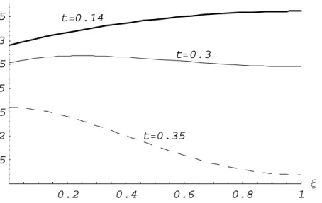
Figure 1 illustrates Proposition 3 when P(Q) = 6−Q, c = 5.6, and n = 10. With this parameter configuration, bt = 0.267 andt1 = 0.347 < a−c= 0.4. Hence, R∗ adopts,
depending upon the value of the tax t, the three possible forms described in Proposition 3. 0.2 0.4 0.6 0.8 1 ξ 0.0175 0.02 0.0225 0.025 0.0275 0.03 0.0325 R t=0.35 t=0.3 t=0.14
Figure 1: Expected government revenue as a function of enforcement ξ
9This result generalizes Cremer and Gahvari (1999), as they onlyfind a negative relation between tax
Finally, observe that our results hold true for any value of n — i.e., that they do not depend on market structure.
References
[1] Bayer, R. and F. Cowell (2006) “Tax Compliance and Firms’ Strategic Interdepen-dence” DARP WP 81, London School of Economics.
[2] Cremer, H. and F. Gahvari (1993) “Tax evasion and optimal commodity taxation”
Journal of Public Economics 50, 261-275.
[3] Cremer, H. and F. Gahvari (1999) “Excise Tax Evasion, Tax Revenue, and Welfare”
Public Finance Review 27, 77-95.
[4] Goerke, L. and M. Runkel (2006) “Profit Tax Evasion under Oligopoly with Endoge-nous Market Structure” National Tax Journal 59, 851-857.
[5] Goerke, L. and M. Runkel (2007) “Tax Evasion and Competition” WP 2104, CESIfo. [6] Marelli, M. and R. Martina (1988) “Tax Evasion and Strategic Behavior of the Firms”
Journal of Public Economics 37, 55-69.
[7] Seade, J. (1985) “Profitable Cost Increases and the Shifting of Taxation: Equilib-rium Responses of Markets in Oligopoly” Warwick Economic Research Papers #260, University of Warwick.
[8] Virmani, A. (1989) “Indirect Tax Evasion and Product Efficiency” Journal of Public Economics 39, 223-237.
[9] Vives, X. (1999)Oligopoly Pricing, The MIT Press: Massachusetts.
Appendix
Proof of Proposition 2
Applying the Implicit Function Theorem, we differentiate (4) and we obtain, using an envelope argument ∂Q∗ ∂ξ = ne∗t (n+ 1)P0(Q∗) +Q∗P00(Q∗). (6) As (n∗+ 1)P0(Q∗) +Q∗P00(Q∗) =P0(Q∗) +n∗[P0(Q∗) +q∗P00(Q∗)]
and, from (3),
P0(Q) +q∗P00(Q)<0,
then10
(n∗+ 1)P0(Q∗) +Q∗P00(Q∗)<0.
This implies that ∂Q∗/∂ξ <0
Proof of Proposition 3
Wheng(e) =e2/2, e∗ = (1−ξ)t.In what follows, we assumet <1/(1−ξ),so interior solutions fore∗ obtain. When P(Q) =a−bQ, first and second derivatives ofP(Q) are
P0(Q) =−bandP00(Q) = 0,
which verify (3). Using(4) and e∗, the equilibrium production is thus given by:
Q∗ = n b(n+ 1) " (a−c)−t à 1− t(1−ξ) 2 2 !# .
Assuming that t < a− c, equilibrium quantities and profits are non negative for any enforcement level ξ. After some manipulation of (5), we obtain
∂R∗
∂ξ =
ne∗t
−b(n+ 1)[M −2(e
∗)2] (7)
where M = 3t−2(a−c). The sign of this derivative is the opposite of the sign of the expression in brackets. On the one hand, when t ≤ bt = 2(a−c)/3, ∂R∗/∂ξ is positive for all ξ. On the other hand, when bt < t < (a−c), ∂R∗/∂ξ is positive (negative) when
ξ ≤ (>)ˆξ = 1−(1/t)pM/2. So R∗ is inverse U-shaped in ξ if ˆξ > 0 and decreasing, if
ˆ
ξ <0.
The conditions for ˆξ >0 (<0)is that the polynomial defined by
Υ(t) = 2t2−3t+ 2 (a−c)
is greater (lower) than 0. Whena−c≤1/2, Υ(t)≥0 if 2(a−c)/3< t≤t1, where t1 =
3−p9−16(a−c) 4
andΥ(t)<0ift1 < t≤(a−c).Whena−c >1/2,Υ(t)≥0for any2(a−c)/3< t < a−c.