Satellite Remote Sensing of Particulate Matter Air Quality:
The Cloud-Cover Problem
Sundar A. Christopher
Earth System Science Center and Department of Atmospheric Sciences, University of Alabama–
Huntsville, Huntsville, AL
Pawan Gupta
Earth System Science Center, University of Alabama–Huntsville, Huntsville, AL
ABSTRACT
Satellite assessments of particulate matter (PM) air quality that use solar reflectance methods are dependent on avail-ability of clear sky; in other words, mass concentrations of PM less than 2.5 m in aerodynamic diameter (PM2.5) cannot be estimated from satellite observations under cloudy conditions or bright surfaces such as snow/ice. Whereas most ground monitors measure PM2.5 concen-trations on an hourly basis regardless of cloud conditions, space-borne sensors can only estimate daytime PM2.5in cloud-free conditions, therefore introducing a bias. In this study, an estimate of this clear-sky bias is provided from monthly to yearly time scales over the continental United States. One year of the Moderate Resolution Imaging Spectroradiometer (MODIS) 550-nm aerosol optical depth (AOD) retrievals from Terra and Aqua satellites, collocated with 371 U.S. Environmental Protection Agency (EPA) ground monitors, have been analyzed. The results indi-cate that the mean differences between PM2.5reported by ground monitors and PM2.5calculated from ground mon-itors during the satellite overpass times during cloud-free conditions are less than⫾2.5g m⫺3, although this value varies by season and location. The mean differences are not significant as calculated byttests (␣ ⫽0.05). On the basis of this analysis, it is concluded that for the conti-nental United States, cloud cover is not a major problem for inferring monthly to yearly PM2.5 from space-borne sensors.
INTRODUCTION
Ground-level or surface pollutants including ozone, car-bon monoxide, sulfur dioxide, nitrogen dioxide, and aerosols are produced from various sources. This paper is focused only on aerosols or particulate matter (PM) less
than 2.5m in aerodynamic diameter (PM2.5), also known as fine or respirable particles. These particles are injected into the atmosphere as primary emissions or form in the atmosphere by gas-to-particle conversion. There are various sources of PM2.5, including emissions from automobiles, industrial exhaust, and vegetation fires. These fine particles have various effects, including reducing visibility; changing surface temperatures by blocking sunlight from reaching the ground; changing cloud properties by acting as cloud con-densation nuclei (CCN)1; and, more importantly, becoming a health hazard.2
Typically PM2.5mass is measured from surface mon-itors, and in the United States there are nearly 600 con-tinuous (hourly) stations managed by federal, state, local, and tribal agencies.3The PM
2.5mass is typically measured by the tapered element oscillating microbalance (TEOM) instrument.4A vibrating hollow tube called the tapered element is set in oscillation at resonant frequency and an electronic feedback system maintains the oscillation am-plitude. When the ambient airstream enters the mass sensor chamber and particulates are collected at the filter, the oscillation frequency of the tapered element changes, and the corresponding mass change is calculated as the change in measured frequency at time t to the initial frequency at time t0. The mass concentration is then calculated from dust mass, time, and flow rate. Ideally, only the collection of aerosol mass on the filter should change the tapered element frequency. However, temper-ature fluctuations, humidity changes, flow pulsation, and change in filter pressure could affect the TEOM perfor-mance. Even in best-case scenarios when the operational parameters can be held constant, the heat-induced loss of volatile material could pose serious errors in the PM2.5 mass.5 However, various correction factors are usually applied to adjust for these factors, although the PM2.5 mass usually represents the lower limits of a true value.5 These ground measurements are invaluable for mea-suring, monitoring, and establishing regulatory policies. The U.S. Environmental Protection Agency (EPA) has es-tablished guidelines for what constitutes good and haz-ardous air quality.3In 1971, EPA issued PM air quality standards that were revised first in 1987 and further in 1997. In 2006, EPA changed the standards for 24-hr aver-aged PM2.5mass values from 65 to 35g m⫺
3primarily on the basis of scientific studies regarding public health.2
IMPLICATIONS
Currently, environmental agencies are interested in using satellite-derived aerosol products to monitor and evaluate PM air quality. These products are only available under cloud-free conditions, which may introduce a bias in long-term evaluation of PM2.5air quality. The effect of cloud
cover on monthly and yearly PM2.5 mass concentration
The ground monitors have obvious advantages. The measurement techniques can be standardized and applied across all locations. They can measure pollution 24 hr/day and provide hourly, daily, monthly, or any type of time average. They can measure pollution regardless of clouds because these are filter-based measurements that are usu-ally fixed at the surface. They also have certain disadvan-tages. The obvious one is that they are point measure-ments and are not representative of pollution over large spatial areas. For example, Huntsville, AL, with an area of approximately of 3223 km2, has only one PM
2.5monitor and therefore it cannot capture pollution in and around the city, nor the gradients in pollution. These ground monitors often miss pollution that is not within the sam-pling area of the measurement. Other cities such as Bir-mingham, AL, have several PM2.5monitors6in the region but are still unable of capturing pollution for every square kilometer. Moreover these ground monitors are expensive and require regular maintenance. Also, the lack of a large-scale picture makes it difficult to assess where the pollu-tion is coming from and where it is heading. The United States has the luxury of having more than 1000 ground monitors,7but most countries have very few or no ground monitors for PM2.5assessments although scientific studies have shown that exposure to high concentrations of PM2.5can affect mortality.2
Satellite Remote Sensing of Aerosol Optical Depth and PM2.5
For every square kilometer of the Earth to be monitored, satellite remote sensing is the only viable method. There are several hundred satellites currently in orbit and not all of them have instruments that are suited for air quality measurements. In their critical review, Hoff and Christo-pher8list the sensors that are especially suited for moni-toring PM air quality. Currently, the workhorse sensor for measuring global pollution from space on a reliable, re-peated basis is the Moderate Resolution Imaging Spectro-radiometer (MODIS). MODIS measures reflected and emit-ted radiance in 36 channels from the ultraviolet to the thermal infrared part of the electromagnetic spectrum. These well-calibrated radiance measurements are con-verted to aerosol optical depth (AOD), which is a measure of the column (surface to top of atmosphere) integrated extinction (absorption plus scattering).8,9Although AOD retrievals from satellites are possible at multiple wave-lengths, this paper refers to the AODs at 550 nm, which are interpolated from 470 and 660 nm. However, these AOD values are only available for cloud-free regions. If the pollution is below the cloud, the satellite cannot “see” this pollution and AOD cannot be inferred. Also, AOD values are not retrieved over bright regions such as snow and ice.
Most satellite-based studies are interested in estimat-ing the PM2.5mass near the ground, whereas the satellites provide a unitless AOD value that is representative of the column.10The column-integrated AOD is related to PM
2.5 mass near the ground, but it requires ancillary informa-tion to estimate the surface PM2.5 from a column mea-surement, such as vertical structure, relative humidity (RH), and other factors.8Perhaps the most critical piece of information is the height of the aerosol layer, because if
the aerosols are lofted above, the ground monitor does not measure a value whereas the satellite will provide an AOD value.11More than 50 papers have examined the use of satellite AOD to infer PM2.5near the surface,8which is not the focus here.
The satellite-based estimates of PM2.5have some ob-vious advantages, including reliable, repeated coverage globally that is indeed cost-effective for monitoring pol-lution. There is nearly a 10-yr record of well-calibrated satellite measurements and validated AOD values over the globe that is freely available. The major disadvantage is that they represent columnar values and require other ancillary pieces of information (e.g., meteorology, height information from space/ground-based lidars) to estimate PM2.5mass values near the ground.8Moreover, the next generation of geostationary satellites will have sensors with improved spectral, temporal, radiometric resolution to tackle the air quality problem in ways that are not possible now.12
It has been shown that under conditions of a well-mixed boundary layer height with low ambient RH, the relationship between PM2.5 and AOD is indeed excellent.10This is especially true for the southeastern United States, where the correlations between hourly PM2.5 mass and satellite AOD are greater than 0.6 and those between daily PM2.5 mass and AOD are greater than 0.9.10,13 On the other hand, these relationships break down if only a two-variate (PM2.5-AOD) regres-sion is performed.14However, when height information coupled with meteorology is used, these relationships can be improved.10,15
The Cloud-Cover Problem
One of the major criticisms of the satellite-based methods is that they can provide AOD and therefore PM2.5 estima-tions only when there are no clouds.16 To address this issue, Gupta and Christopher17 calculated PM
2.5 mass from daily ground measurements (PM2.5) from monthly to yearly time scales (ALLPM) and compared these against the same ground-measurements only for those days when satellite data are available for clear-sky conditions (CLEARPM). It is important to note that they did not use the satellite-derived AOD; they simply used the PM2.5 from the ground monitors during the time of the satellite overpass when MODIS did not report clouds. They re-ported these results over 38 ground monitors over the southeastern United States and concluded that although satellite data are generally available less than 50% of the time, mean differences between ALLPM and CLEARPM over monthly to yearly time scales is less than 2g m⫺3, indicating that low sampling from satellites due to cloud cover and other reasons (e.g., bright snow/ice surfaces) is not a major problem for studies that require long-term PM2.5datasets. This means that on a certain day, over a location, the satellite may not provide a PM2.5mass value, but over monthly to yearly time scales the mean differ-ence between the values averaged by the ground monitor and the satellite is within 2g m⫺3, although this value can be higher over certain locations depending on vari-ability in PM2.5mass. This is especially important because long-term exposure studies require global datasets on longer time scales,2and it is important to know the utility
of satellite data, especially because they are not used in cloudy conditions.
Because analyzing only the southeastern United States limits the applicability of the results to other re-gions, this paper analyzed data from nearly 371 ground monitors over the entire United States to see if cloud cover poses a problem for reporting long-term (in this case monthly to yearly time scales) PM2.5statistics. Data from only 371 of the more than 600 ground monitors are used because of sampling issues that are explained in the sectionStudy Area, Data, and Methods. The questions asked are still the same as those posed by Gupta and Christo-pher,17except that they are analyzed for the entire United States for all seasons, which represents a wide range of surface and climate regimes. The questions are as follows: What is the difference between ground-based PM2.5 (ALLPM) and the PM2.5 for only those days in which satellite data are available (CLEARPM) on monthly and yearly time scales? How many days of satellite data are available because of cloud-cover contamination and other limitations for PM2.5air quality research?
STUDY AREA, DATA, AND METHODS
To analyze these differences, the United States were cate-gorized by 10 EPA zones (Figure 1) that have several unique aerosol types and climate regimes.18 Twenty-four-hour average PM2.5mass concentration values were used from 600 ground monitoring stations (Figure 2) from January 1, 2006 to December 31, 2006, covering the entire continental United States. These daily PM2.5values were
first used to calculate monthly means (ALLPM). Terra and Aqua MODIS satellite data (MODO4 and MYD04, Collec-tion 5, respectively)19were obtained that contained AOD and other geophysical parameters in 10- by 10-km2spatial resolution. The Terra and Aqua overpasses occur at ap-proximately 10:30 a.m. and 1:30 p.m. local time, respec-tively. The MODIS AOD data are available for cloud-free conditions and retrieval is performed when surface reflec-tance in the 2.1-m channel is less than 0.4. The MODIS algorithm also considers the retrieved AOD as question-able if the 2.1-m channel reflectance is more than 0.25.19 For each one of the PM2.5ground monitors, a 5⫻5 group of the 10- by 10-km2 MODIS pixels centered on the ground monitor is examined. This method of using 5⫻5 pixels is often the standard practice when comparing ground-based with satellite measurements.13 The spatial resolution of one MODIS AOD pixel is approximately 10 ⫻ 10 km2, whereas surface measurements are point values, which makes intercomparisons difficult. Even if the MODIS pixel was small enough, it does not represent the same viewing conditions because of differences be-tween observation areas and varying path lengths through the atmosphere. Averaging level 2 MODIS AOD pixels using a 5- by 5-pixel box over the ground monitors and 15-min observations over 1 hr represents a similar air mass as observed by MODIS. Only the satellite data were used to check if AOD retrievals are available for the 5- by 5-pixel grid. Even if one of the pixels in the 5⫻5 grid had a reported AOD value, the ground-based PM2.5for these days are tagged and labeled as CLEARPM, because this is what MODIS will sample over time. If MODIS-retrieved
Figure 1. The center of the figure shows the EPA regions in various colors with the EPA regions marked from 1 to 10. The 10 panels surrounding show the number of days available from MODIS for estimating PM2.5shown as connected lines (0 –100%), the ALLPM-CLEARPM
AOD is present on any given day over the ground loca-tion, the PM2.5 value from the ground was included in computing monthly means and is referred to as CLEARPM. Note that the satellite-derived AOD values are not used in the calculations. In this way, the difference between mean PM2.5values from the all-ground measure-ments (ALLPM) and PM2.5values from only those ground measurements for which the satellite-derived AOD values are available (CLEARPM) were measured. Also tracked were the number of days when satellite data are available in a given month, season, or year (referred to as SATDAYS throughout the paper). For example, if a 5⫻ 5 grid had reported AOD values for every single day in an entire month, then it would indicate that there was 100% data availability from the satellite during that month. For all of the following analysis, 85% thresholds were set on data availability from the surface data to maintain uniformity across all locations. For seasonal analysis 75 of 90 days, and for monthly analysis 25 of 30 days, corresponding to approximately 85% data availability, were used. Although there are more than 600 AirNow sites across the United States, because of this strict criterion, data from only 371 ground monitors were used. The Terra and Aqua satellites were used to assess if there are differences between ALLPM and CLEARPM due to differences in overpass time. RESULTS AND DISCUSSION
Figure 1 shows the 10 EPA regions in various colors in the center. Each surrounding panel represents an EPA region
and shows the number of days available from MODIS over each EPA region for each month (SATDAYS), which are shown as connected lines (secondaryy-axis). Also shown in each panel is the mean difference between ALLPM and CLEARPM for each month and the standard deviations within that EPA region. The number of ground monitors and the mean SATDAYS for each EPA region are also indicated. For example, for EPA region 4 (southeastern United States), the highest numbers of SATDAYS are dur-ing sprdur-ing and summer months, with slightly lower val-ues available during the winter season. However, the sea-sonal ALLPM-CLEARPM (Table 1) ranges from⫺0.26 to 1.18g m⫺3, indicating that there is very little sampling bias due to missing days when cloud cover (and snow/ice backgrounds) did not allow MODIS to obtain aerosol ob-servations. Several interesting features can be seen in Fig-ure 1. The number of ground monitors is not constant among the EPA regions. Note that only those ground monitors have been used where 85% of MODIS measure-ments are available. EPA regions 7 and 8 have only 15–17 monitors, whereas EPA region 4 (southeast) has the high-est number of ground monitors (73). Although the selec-tion of locaselec-tions of ground monitors may be concentrated more in urban locations, EPA regions 7 and 8 often expe-rience a high level of transported pollutants from biomass burning smoke from Canada20 that are currently not monitored because of the lack of ground observations. Satellite remote sensing in this case can be a cost-effective option for monitoring PM pollution, especially those transported from outside of the continental United States. In general, spring and summer months are the best for monitoring pollution from space. Some regions have a large month-to-month variation in SATDAYS primarily because of cloud/snow cover issues. For example EPA re-gion 3 (northeast) has less than 10% SATDAYS (⬃3 days per month), whereas the drier climate of EPA region 9 allows for more SATDAYS, although some areas may not have AOD retrievals because of high surface reflectance and other retrieval limitations.
In general, ALLPM-CLEARPM should be largest when SATDAYS is low because fewer numbers of days for sam-pling produces larger standard deviations. This can be seen in almost all EPA regions (Figure 1) where winter months have the lowest number of SATDAYS and the corresponding differences in ALLPM and CLEARPM are higher, except in the case of EPA regions 4 and 6 where differences are higher during summer and fall seasons although SATDAYS are also high. However, there are some exceptions (EPA regions 4 and 6) because the value of ALLPM-CLEARPM may also depend more on day-to-day variability in PM2.5mass concentration in any given month associated with increased production of secondary aerosols due to enhanced photochemistry during summer months. This daily variability is a function of location, or, more precisely, the type and/or sources of aerosols that cannot be assessed from these datasets. The value of ALLPM-CLEARPM will be low for regions and seasons where day-to-day variability is lower compared with high-variability regions and seasons. Even low numbers of SAT-DAYS in a region of low variability in PM2.5should pro-duce a smaller difference in ALLPM and CLEARPM. This can be seen in EPA region 1 during the winter season Figure 2. The difference between the annual mean
ALLPM-CLEARPM ing m⫺3for each PM
2.5ground monitor for (a) Aqua
(Table 1) where only 12% of days’ satellite data were available but the difference in ALLPM and CLEARPM was almost negligible (0.01g m⫺3). However, during other seasons in the same EPA region, SATDAYS are high enough (spring, 28%; summer, 34%; fall, 21%) but still the difference in ALLPM and CLEARPM is much larger (⬃2 g m⫺3), which clearly indicates the difference in variability in surface PM2.5 mass concentration in the same region during different seasons. Table 1 provides the mean and standard deviation of ALLPM, CLEARPM, MO-DIS AOD, and SATDAYS as a function of season and EPA region. Two sample (ALLPM and CLEARPM)t tests were performed for each region with the null hypothesis ALLPM⫺ CLEARPM⫽0 for␣ ⫽0.05. These results indi-cate that the differences are statistically not significant and therefore the null hypothesis was not rejected. Figure
2 shows the locations of the ground monitors and the yearly mean ALLPM-CLEARPM differences for each loca-tion in micrograms per cubic meter. These differences are also shown for Aqua (Figure 2a) and Terra (Figure 2b). The results can be interpreted along with information from Table 2 that shows the seasonal numbers for each EPA region. Although there are some differences between the Aqua and Terra in Figure 2, for the most part, the ALLPM-CLEARPM differences are not very different between the two sensors. Rather than focusing on individual loca-tions, these differences are assessed as a function of EPA region. Smaller differences are seen in the southeast, whereas some locations in the northeast and west have higher differences primarily because of issues related to cloud cover. One of the largest seasonal changes in cloud cover is seen in EPA region 10 (northwest), which varies
Table 1. Statistics for all relevant parameters used in this study for each EPA region and for each season.
Season EPA Region ALLPMa
ALLPM b CLEARPMc CLEARPM d AODe AOD f ALLPM-CLEARPM SATDAY (%) Winter 1 10.56 2.42 10.55 4.35 0.12 0.06 0.01 12 2 10.47 2.27 12.09 3.16 0.19 0.08 ⫺1.62 14 3 11.99 3.27 12.72 4.97 0.11 0.05 ⫺0.73 19 4 10.59 2.07 10.85 2.59 0.08 0.05 ⫺0.26 35 5 12.72 4.18 13.98 5.57 0.20 0.08 ⫺1.26 22 6 8.12 3.56 8.03 3.54 0.10 0.05 0.09 31 7 9.45 2.43 9.02 2.72 0.13 0.05 0.43 25 8 9.92 3.36 9.61 5.40 0.20 0.10 0.31 13 9 17.49 7.97 18.92 10.72 0.14 0.09 ⫺1.43 36 10 9.75 3.22 11.45 5.95 0.09 0.09 ⫺1.7 16 Spring 1 7.37 2.03 9.83 3.97 0.17 0.09 ⫺2.46 28 2 7.77 2.04 9.16 3.37 0.20 0.08 ⫺1.39 34 3 12.37 2.78 12.48 4.33 0.17 0.05 ⫺0.11 51 4 14.07 1.94 14.31 2.41 0.17 0.06 ⫺0.24 52 5 12.20 3.85 12.58 4.98 0.23 0.09 ⫺0.38 37 6 11.15 4.09 10.90 4.01 0.18 0.06 0.25 40 7 10.83 2.27 10.69 2.55 0.20 0.09 0.14 36 8 7.43 2.54 8.19 2.81 0.26 0.10 ⫺0.76 39 9 10.92 5.44 11.80 5.85 0.25 0.15 ⫺0.88 45 10 5.65 1.50 6.47 2.08 0.13 0.07 ⫺0.82 36 Summer 1 11.61 3.66 13.34 3.90 0.23 0.10 ⫺1.73 34 2 13.39 4.92 15.37 4.90 0.30 0.11 ⫺1.98 36 3 20.65 4.66 22.60 4.99 0.32 0.09 ⫺1.95 51 4 19.38 4.00 21.25 4.41 0.37 0.11 ⫺1.87 54 5 15.46 5.04 15.20 5.52 0.24 0.09 0.26 49 6 12.59 4.78 13.03 5.21 0.22 0.08 ⫺0.44 48 7 13.10 3.15 13.54 3.64 0.19 0.05 ⫺0.44 55 8 9.36 3.28 9.34 3.44 0.22 0.09 0.02 65 9 13.67 5.87 13.76 5.89 0.25 0.17 ⫺0.09 75 10 6.57 3.18 7.05 3.11 0.13 0.07 ⫺0.48 74 Fall 1 8.36 2.58 10.19 3.56 0.13 0.06 ⫺1.83 21 2 9.81 3.42 11.82 3.96 0.17 0.10 ⫺2.01 22 3 13.65 3.64 15.35 4.39 0.14 0.09 ⫺1.7 36 4 12.78 2.64 13.91 2.76 0.12 0.07 ⫺1.13 46 5 12.16 4.12 12.85 4.31 0.15 0.07 ⫺0.69 27 6 9.65 3.79 9.89 4.21 0.11 0.06 ⫺0.24 47 7 9.60 3.09 9.50 2.87 0.11 0.06 0.1 39 8 8.36 3.05 8.97 2.93 0.15 0.07 ⫺0.6 37 9 14.95 6.45 14.81 6.26 0.18 0.10 0.14 60 10 9.61 3.29 10.15 3.79 0.14 0.11 ⫺0.54 55
Notes:aALLPM is mean PM
2.5from ground monitor that uses all data;bALLPMis the ALLPM standard deviation;cCLEARPM is the PM2.5calculated only during
the satellite overpass when there were no clouds;d
CLEARPMis the standard deviation for CLEARPM;eAOD is MODIS AOD at 550 nm;fAODis the standard deviation
from 16 to 74% through the year. The ALLPM-CLEARPM differences range from⫺0.48 to⫺1.74g m⫺3. In com-parison, EPA region 4 (southeast) has smaller changes in cloud cover as a function of season (35–54%), and ALLPM-CLEARPM differences are between ⫺0.24 and ⫺1.87 g m⫺3. Note the seasonality in Table 1 in the ALLPM columns where the ALLPM values are high across most EPA regions during summer and vary markedly across regions during the winter months because of me-teorological factors such temperature and precipitation (not shown). Remarkably, the ALLPM-CLEARPM differ-ences are less than 2g m⫺3for every region and every season except during spring for EPA region 1, where a value of⫺2.5g m⫺3was calculated because of the high cloud cover in this region.
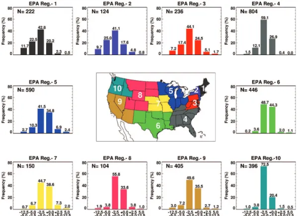
Figure 3 shows some of the key results from this work using the frequency distribution of ALLPM-CLEARPM as a function of the 10 EPA regions. The overall frequency of ALLPM-CLEARPM is negative, which indicates that the PM2.5calculated during the time of the satellite overpass is missing days with lower daily PM2.5 mass concentra-tion, making the differences negative. In general, clear sky conditions are quite often associated with low wind speed, sinking air motion, reduced vertical mixing, and enhanced photochemistry. These conditions result in ac-cumulation of pollutants at the ground, and the reverse is true for cloudy conditions when satellite observations of aerosols are not possible. This explains the negative dif-ferences between ALLPM and CLEARPM due to cloud cover. However, during winter at high latitudes, surface snow cover provides another limitation to aerosol re-trieval from the satellite observations because the MODIS
Collection 5 aerosol retrieval algorithm largely follows the dark target approach.19 Figure 3 clearly shows that negative ALLPM-CLEARPM differences occurred during the dry and hotter months, whereas positive differences occurred during the colder months. Except for EPA re-gions 1, 2, and 3, more than 80% of the differences are within ⫾2.5 g m⫺3. These results provide tremendous confidence for using satellite data for assessing PM2.5 al-though cloud/snow cover prohibits measurements nearly 50% of the time. To reiterate, this does not mean that the AOD and PM2.5are well correlated. The authors simply note that for long-term averages from monthly to yearly time scales, cloud/snow cover sampling biases only intro-duce a mean uncertainty of approximately⫾2.5g m⫺3. CONCLUSIONS
Space-borne sensors can only provide an estimate of PM2.5 when there are no clouds obstructing their view, whereas ground monitors measure PM2.5mass concentra-tions regardless of cloud cover. This study analyzed 1 yr of Terra-MODIS and Aqua-MODIS satellite data in conjunc-tion with nearly 400 ground monitors of PM2.5to answer the following question: What is the difference between PM2.5 mass measured by the ground monitor and the PM2.5mass measured at the ground only during the times when there was no cloud cover sensed by the satellite? Quantifying this is important because if satellites are to be used to assess PM2.5 near the ground, how much the PM2.5biases are due to missed opportunities because of clouds needs to be known. These results indicate that over 371 ground monitors the mean differences are within 2.5 g m⫺3. It is therefore concluded that if the satellite AOD
Figure 3. The center of the figure shows the EPA regions in various colors with the EPA regions marked from 1 to 10. The 10 panels surrounding show the frequency distribution of ALLPM-CLEARPM for the 10 EPA zones.
can be appropriately used to estimate PM2.5 near the ground, then clouds do not pose a major problem for estimating monthly to yearly PM2.5mass concentrations that are critical for long-term exposure studies.
ACKNOWLEDGMENTS
This research was sponsored by National Oceanic and Atmospheric Administration air quality projects at the University of Alabama–Huntsville. MODIS data were ob-tained from the Level 1 and Atmosphere Archive and Distribution System at the Goddard Space Flight Center. PM2.5data were obtained from EPA’s Air Quality System. REFERENCES
1. Kaufman, Y.J.; Tanre, D.; Boucher, O. A Satellite View of Aerosols in the Climate System;Nature2002,419, 215-223.
2. Pope, C.A., III; Dockery, D.W. Health Effects of Fine Particulate Air Pollution: Lines that Connect;J. Air & Waste Manage. Assoc.2006,56, 709-742.
3. Ambient Air Monitoring Strategy for State, Local, and Tribal Air Agencies; U.S. Environmental Protection Agency; Office of Air Quality Planning and Standards: Research Triangle Park, NC, 2008.
4. Lee, J.H.; Hopke, P.K.; Holsen, T.M.; Polissar, A. Evaluation of Contin-uous and Filter-Based Methods for Measuring PM2.5Mass
Concentra-tion;Aerosol Sci. Technol.2005,39, 290-303.
5. Grover, B.D.; Kleinman, M.; Eatough, N.L.; Eatough, D.J.; Hopke, P.K.; Long, R.W.; Wilson, W.E.; Meyer, M.B.; Ambs, J.L. Measurement of Total PM2.5Mass (Nonvolatile Plus Semivolatile) with the Filter
Dy-namic Measurement System Tapered Element Oscillating Microbal-ance Monitor; J. Geophys. Res. 2005, 110, D07S03; doi: 10.1029/ 2004JD004995.
6. Wang, J.; Christopher, S.A. Intercomparison between Satellite-Derived Aerosol Optical Thickness and PM2.5Mass: Implications for Air
Qual-ity Studies; Geophys. Res. Lett. 2003, 30, 2095; doi: 10.1029/ 2003GL018174.
7. Al-Saadi, J.; Szykman, J.; Pierce, R.B.; Kittaka, C.; Neil, D.; Chu, D.A.; Remer, L.; Gumley, L.; Prins, E.; Weinstock, L.; Macdonald, C.; Way-land, R.; Dimmick, F.; Fishman, J. Improving National Air Quality Forecasts with Satellite Aerosol Observations;Bull. Am. Meteorol. Soc. 2005,86, 1249-1261.
8. Hoff, R.; Christopher, S.A. Remote Sensing of Particulate Matter Air Pollution from Space: Have We Reached the Promised Land;J. Air & Waste Manage. Assoc. 2009, 59, 645-675; doi: 10.3155/1047-3289.59.6.645.
9. Remer, L.A.; Kaufman, Y.J.; Tanre´, D.; Mattoo, S.; Chu, D.A.; Martins, J.V.; Li, R.-R.; Ichoku, C.; Levy, R.C.; Kleidman, R.G.; Eck, T.F.; Ver-mote, E.; Holben, B.N. The MODIS Aerosol Algorithm, Products and Validation;J. Atmos. Sci.2005,62, 947-973.
10. Gupta, P.; Christopher, S.A. Particulate Matter Air Quality Assessment Using Integrated Surface, Satellite, and Meteorological Products: Mul-tiple Regression Approach;J. Geophys. Res.2009,114, D14205; doi: 10.1029/2008JD011496.
11. Engel-Cox, J.A.; Hoff, R.M.; Rogers, R.; Dimmick, F.; Rush, A.C.; Szyk-man, J.J.; Al-Saadi, J.; Chu, D.A.; Zell, E.R. Integrating Lidar and Sat-ellite Optical Depth with Ambient Monitoring for 3-Dimensional Par-ticulate Characterization;Atmos. Environ.2006,40, 8056-8067; doi: 10.1016/j.atmosenv.2006.02.039.
12.Geostationary Coastal and Air Pollution Events; Workshop Report; Na-tional Aeronautics and Space Administration: Chapel Hill, NC, 2008. 13. Gupta, P.; Christopher, S.A. Seven Year Particulate Matter Air Quality Assessment from Surface and Satellite Measurements;Atmos. Chem. Phys. Discuss.2008,8, 3311-3324.
14. Engel-Cox, J.A.; Christopher, H.H.; Coutant, B.W.; Hoff, R.M. Quali-tative and QuantiQuali-tative Evaluation of MODIS Satellite Sensor Data for Regional and Urban Scale Air Quality;Atmos. Environ.2004,38, 2495-2509.
15. Liu, Y.; Park, R.J.; Jacob, D.J.; Li, Q.; Kilaru, V.; Sarnat, J.A. Mapping Surface Concentrations of Fine Particulate Matter Using MISR Satellite Observations of Aerosol Optical Thickness;J. Geophys. Res.2004,109, D22206; doi: 10.1029/2004JD005025.
16. Hidy, G. Introduction to the 2009 Critical Review: Remote Sensing of Particulate Pollution from Space: Have We Reached the Promised Land?;J. Air & Waste Manage.Assoc.2009,59, 642-644; doi: 10.3155/ 1047-3289.59.6.642.
17. Gupta, P.; Christopher, S.A. An Evaluation of Terra-MODIS Sampling for Monthly and Annual Particulate Matter Air Quality Assessment over the Southeastern United States;Atmos. Environ.2008,42, 6465-6471.
18. Malm, W.C.; Sisler, J.F.; Huffman, D.; Eldred, R.A.; Cahill, T.A. Spatial and Seasonal Trends in Particle Concentration and Optical Extinction in the United States;J. Geophys. Res.1994,99, 1347-1370.
19. Levy, R.C.; Remer, L.A.; Mattoo, S.; Vermote, E.F.; Kaufman, Y.J. Second-Generation Operational Algorithm: Retrieval of Aerosol Prop-erties over Land from Inversion of Moderate Resolution Imaging Spec-troradiometer Spectral Reflectance; J. Geophys. Res. 2007, 112, D13211; doi: 10.1029/2006JD007811.
20. Colarco, P.R.; Schoeberl, M.R.; Doddridge, B.G.; Marufu, L.T.; Torres, O.; Welton, E.J. Transport of Smoke from Canadian Forest Fires to the Surface near Washington, D.C.: Injection Height, Entrainment, and Optical Properties;J. Geophys. Res.2004,109, D06203; doi: 10.1029/ 2003JD004248.
About the Authors
Sundar A. Christopher is a professor and associate director at the Earth System Science Center and Department of Atmospheric Sciences at the University of Alabama–Hunts-ville. Pawan Gupta is a research scientist with the Earth System Science Center at the University of Alabama– Huntsville. Please address correspondence to: Sundar Christopher, University of Alabama–Huntsville, Alabama Campus, Huntsville, AL 35805; phone:⫹1-256-961-7872; fax:⫹1-256-961-7755; e-mail: [email protected].