Computers & Graphics 31 (2007) 157–174
A fast all nearest neighbor algorithm for applications
involving large point-clouds
Jagan Sankaranarayanan
, Hanan Samet, Amitabh Varshney
Department of Computer Science, Center for Automation Research, Institute for Advanced Computer Studies,University of Maryland, College Park, MD - 20742, USA
Abstract
Algorithms that use point-cloud models make heavy use of the neighborhoods of the points. These neighborhoods are used to compute the surface normals for each point, mollification, and noise removal. All of these primitive operations require the seemingly repetitive process of finding theknearest neighbors (kNNs) of each point. These algorithms are primarily designed to run in main memory. However, rapid advances in scanning technologies have made available point-cloud models that are too large to fit in the main memory of a computer. This calls for more efficient methods of computing thekNNs of a large collection of points many of which are already in close proximity. A fastkNNalgorithm is presented that makes use of the locality of successive points whoseknearest neighbors are sought to reduce significantly the time needed to compute the neighborhood needed for the primitive operation as well as enable it to operate in an environment where the data is on disk. Results of experiments demonstrate anorderof magnitude improvement in thetimeto perform the algorithm andseveral ordersof magnitude improvement inwork efficiencywhen compared with several prominent existing methods. r2006 Elsevier Ltd. All rights reserved.
MSC:68U05
Keywords:Neighbor finding;kNearest neighbors;kNNAlgorithm; All nearest neighbor algorithm; Incremental neighbor finding algorithm; Locality; Neighborhood; Disk-based data structures; Point-cloud operations; Point-cloud graphics
1. Introduction
In recent years there has been a marked shift from the use of triangles to the use of points as object modeling primitives in computer graphics applications (e.g.,[1–5]). A point model (often referred to as a point-cloud) usually contains millions of points. Improved scanning technolo-gies[4]have resulted in enabling even larger objects to be scanned into point-clouds. Note that a point-cloud is nothing more than a collection of scanned points and may not even contain any topological information. However, most of the topological information can be deduced by
applying suitable algorithms on the point-clouds. Some of the fundamental operations performed on a freshly scanned point-cloud include the computation of surface normals in order to be able to illuminate the scanned object, applica-tions of noise-filtersto remove any residual noise from the scanning process, and tools that change thesampling rateof the point model to the desired level. What is common to all three of these operations is that they work by computing the knearest neighbors for each point in the point-cloud. There are two important distinctions from other applications where the computation of neighbors is required. First of all, neighbors need to be computed for all points in the data set, potentially this task can be optimized. Second, no assump-tion can be made about the size of the data set. In this paper, we focus on a solution to the k-nearest-neighbor (kNN) problem, also known as the all-pointskNNproblem, which takes a point-cloud data setRas an input and computes the kNNfor each point inR.
www.elsevier.com/locate/cag
0097-8493/$ - see front matterr2006 Elsevier Ltd. All rights reserved. doi:10.1016/j.cag.2006.11.011
Corresponding author. Tel.: +1 301 405 1769; fax: +1 301 314 9115.
E-mail addresses:[email protected] (J. Sankaranarayanan), [email protected] (H. Samet),[email protected] (A. Varshney).
URLs: http://www.cs.umd.edu/jagan, http://www.cs.umd.edu/hjs, http://www.cs.umd.edu/varshney.
We start by comparing and contrasting our work with the related work of Clarkson[6]and Vaidya[7]. Clarkson proposed anOðnlogdÞalgorithm for computing the nearest
neighbor to each ofnpoints in a data setS, wheredis the
ratio of the diameter of S and the distance between the closest pair of points in S. Clarkson uses a PR quadtree (e.g., see[8])Qon the points inS. The running time of his algorithm depends on the depth d¼d of Q. This
dependence on the depth is removed by Vaidya who proposed using a hierarchy of boxes, termed a Box tree, to compute the kNNs to each of the n points in S in
OðknlognÞtime. There are two key differences between our algorithm and those of Clarkson and Vaidya. First of all, our algorithm can work on most disk-based (out of core) data structures regardless of whether they are based on a regular decomposition of the underlying space such as a quadtree[8]or on object hierarchies such as an R-tree[9]. In contrast to our algorithm, the methods of Clarkson and Vaidya have only been applied to memory-based (i.e., incore) data structures such as the PR quadtree and Box tree, respectively. Consequently, their approaches are limited by the amount of physical memory present in the computer on which they are executed. The second difference is that it is easy to modify our algorithm to produce nearest neighbors incrementally, i.e., we are able to provide a variable number of nearest neighbors to each point in Sdepending on a condition, which is specified at run-time. The incremental behavior has important applica-tions in computer graphics. For example, the number of neighbors used in computing the normal to a point in a point-cloud can be made to depend on the curvature of a point.
The development of efficient algorithms for finding the nearest neighbors for a single point or a small collection of points has been an active area of research[10,11]. The most prominent neighbor finding algorithms are variants of depth-first search (DFS)[11]or best-first search (BFS)[10]
methods to compute neighbors. Both algorithms make use of a search hierarchy which is a spatial data-structure such as an R-tree[9]or a variant of a quadtree or octree (e.g.,
[8]). The DFS algorithm, also known as branch-and-bound, traverses the elements of the search hierarchy in a predefined order and keeps track of the closest objects to the query point that have been encountered. On the other hand, the BFS algorithm traverses the elements of the search hierarchy in an order defined by their distance from the query point. The BFS algorithm that we use[10], stores both points and blocks in a priority queue. It retrieves points in an increasing order of their distance from the query point. This algorithm isincrementalas the number of nearest neighbors k need not be known in advance. Successive neighbors are obtained as points are removed from the priority queue. A brute force method to perform the kNNalgorithm would be to compute the distance between every pair of points in the data set and then to choose the top k results for each point. Alternatively, we also observe that repeated application of a neighbor finding
technique[12]on each point in the data set also amounts to performing a kNNalgorithm. However, like the brute-force method, such an algorithm performs wasteful repeated work as points in proximity share neighbors and ideally it is desirable to avoid recomputing these neighbors. Some of the work entailed in computing thekNNs can be reduced by making use of the approximate nearest neighbors (ANNs)[12]. In this case, the approximation is achieved by making use of an error-boundwhich restricts the ratio of the distance from the query point q to an approximate neighbor and the distance to the actual neighbor to be within 1þ. When used in the context of a point-cloud algorithm, this method may lead to inaccuracies in the final result. In particular, point-cloud algorithms that determine local surface properties by analyzing the points in the neighborhood may be sensitive to such inaccuracies. For example, such problems can arise in algorithms for computing normals, estimating local curvature, as well as sampling rate and local point-cloud operators such as noise-filtering [3,13], mollification and removal of outliers [14]. In general, the correct computa-tion of neighbors is important in two main classes of point-cloud algorithms: algorithms that identify or compute properties that are common to all of the points in the neighborhood, and algorithms that study variations of some of these properties.
An important consideration when dealing with point models that is often ignored is the size of the point-cloud data sets. The models are scanned at ahigh fidelityin order to create an illusion of a smooth surface. The resultant point models can be on the order of several millions of points in size. Existing algorithms such as normal computation[15]which make use of the suite of algorithms and data structures in the ANN library[12]are limited by the amount of physical memory present in the computer on which they are executed. This is because the ANN library makes use of in-core data structures such as the k-d tree
[16] and the BBD-tree [17]. As larger objects are being converted to point models, there is a need to examine neighborhood finding techniques that work with data that is out of core and thus out-of-core data structures should be used. Of course, although the drawback of out-of-core methods is the incurrence ofI=O costs, thereby reducing their attractiveness for real-time processing, the fact that most of the techniques that involve point-clouds are performedofflinemitigates this drawback.
There has been a considerable amount of work on efficient disk-based nearest neighbor finding methods
[10,11,18]. Recently, there has also been some work on thekNNalgorithm[18,19]. In particular, the algorithm by Bo¨hm [19], termed MuX uses the DFS algorithm to compute the neighborhoods of one block, sayb, at a time (i.e., it computes the kNNs of all points in b before proceeding to compute the kNNs in other blocks) by maintaining and updating a best set of neighbors for each point in the block as the algorithm progresses. The rationale is that this will minimize diskI=Oas the KNNs
of points in the same block are likely to be in the same set of blocks. TheGORDERmethod[18]takes a slightly different approach in that although it was originally designed for high-dimensional data-points (e.g., similarity retrieval in image processing applications), it can also be applied to low-dimensional data sets. In particular, this algorithm first performs a principal component analysis (PCA) to determine the first few dominant directions in the data space and then all of the objects are projected to this dimensionally reduced space, thereby resulting in drastic reduction in the dimensionality of the point data set. The resulting blocks are organized using a regular grid, and, at this point, akNNalgorithm is performed which is really a sequential search of the blocks.
Even though both the GORDER [18] and the MuX [19] methods compute the neighborhood of all points in a block before proceeding to process points in another block, each point in the block keeps track of itskNNs encountered thus far. Thus this work is performed independently and in isolation by each point with no reuse of neighbors of one point as neighbors of a point in spatial proximity. Instead, in our approach we identify a region inspacethat contains all of thekNNs of acollectionof points (the space is termed
locality). Once the best possiblelocalityis built, each point searches only the locality for the correct set of k nearest neighbors. This results in large savings. Also, our method makes no assumption about the size of the data set or the sampling-rate of the data. Experiments (Section 6) show that our algorithm is faster than both theGORDER and the MuX methods and performs substantially fewer distance computations.
The rest of the paper is organized as follows. Section 2 defines the concepts that we use and provides a high level description of our algorithm. Section 3 describes the
localitybuilding process forblocks. Section 4 describes an incremental variant of ourkNNalgorithm, while Section 5 describes a non-incremental variant of ourkNNalgorithm. Section 6 presents the results of our experiments, while Section 7 discusses related applications that can benefit from the use of our algorithm. Finally, concluding remarks are drawn in Section 8.
2. Preliminaries
In this paper we assume that the data consists of points in a multi-dimensional space and that they are represented by a hierarchical spatial data structure. Our algorithm makes use of a disk-based quadtree variant that recursively decomposes the underlying space into blocks until the number of points in a block is less than some bucket capacity B[8]. In fact, any other hierarchical spatial data structure could be used including some that are based on object hierarchies such as the R-tree [9]. The blocks are represented as nodes in a tree access structure which enables point query searching in time proportional to the logarithm of the width of the underlying space. The tree contains two types of nodes: leaf and leaf. Each
non-leaf node has at most 2d non-empty children, where d
corresponds to the dimension of the underlying space. A
childnode occupies a region in space that is fully contained in its parent node. Each leaf node contains a pointer to a
bucketthat stores at mostBpoints. Therootof the tree is a special block that corresponds to the entire underlying space which contains the data set. While the blocks of the access structure are stored in main-memory, the buckets that contain the points are stored on disk. In our implementation, a count is maintained of the number of points that are contained within the subtreeof which the corresponding blockbis the root and aminimum bounding box of the space occupied by the points thatbcontains.
We use the Euclidean metric (L2) for computing distances. It is easy to modify our kNNalgorithm to accommodate other distance metrics. Our implementation makes extensive use of the two distance estimates MinDist
and MaxDist (Fig. 1). Given two blocks q and s, the
procedure MinDistðq;sÞ computes the minimum possible
distance between a point inqto a point ins. When a list of blocks is ordered by their MinDistvalue with respect to a
reference block or a point, the ordering is called a MinDist
ordering. Given two blocks q and s, the procedure MaxDistðq;sÞ computes the maximum possible distance
between a point inqto a point ins. When a list of blocks is ordered by their An ordering based on MaxDistis called a
MaxDist ordering. The kNNalgorithm identifies the k
nearest neighbors for each point in the data set. We refer to the set ofkNNs of a pointpas theneighborhoodofp. While the neighborhood is used in the context of points, locality
defines a neighborhood of blocks. Intuitively, the locality of a block b is the region in space that contains all the
kNNs of all points in b. We make one other distinction between the concepts of neighborhood and locality. In particular, while neighborhoods contain no other points other than thekNNs locality is more of an approximation and thus the locality of a blockbmay contain points that do not belong to the neighborhood of any of the points contained withinb.
Our algorithm has the following high-level structure. It first builds the locality for a block and later searches the locality to construct a neighborhood for each point contained within the block. The pseudo-code presented in Algorithm 1 explains the high level workings of the
kNNalgorithm. Lines 1–2 compute the locality of the blocks in the search hierarchyQon the input point-cloud.
MINDIST MAXDIST
q s
Fig. 1. Example illustrating the values of the MinDistand MaxDist distance estimates for blocksqandb.
Lines 3–4 build a neighborhood for each point in b using the locality ofb.
Algorithm 1
ProcedurekNN½Q;k
Input:Qis the search hierarchy on the input point-cloud (high-level description ofkNNalgorithm)
1. foreach blockbin Qdo 2. Buildlocality Sforb inQ
3. for each pointp inb do
4. Buildneighborhoodofp usingSandk
5. end-for 6. end-for 7. return
3. Building the locality of a block
As the locality defines a region in space, we need a measure that defines the extent of the locality. Given aquery block, such a measure would implicitly determine if a point or a block belongs to the locality. We specify the extent of a locality by a distance-based measure that we call PruneDist. All points and blocks whose distance from the query block is less than PruneDistbelong to the locality. The challenge in building localities is to find a good estimate for PruneDist. Finding the smallest possible value of PruneDist requires that we examine every point which defeats the purpose of our algorithm which is why we resort to estimating it.
We proceed as follows. Assume that the query blockqis in the vicinity of other blocks of various sizes. We want to find a set of blocks so that the total number of points that they contain is at leastk, while keeping PruneDistas small as possible. We do this by processing the blocks in increasing order of their MaxDist order from q and adding them to the locality. In particular, we sum the counts of the number of points in the blocks until the total number of points in the blocks that have been encountered exceeds k and record the current value of MaxDist as the value of PruneDist. At this point, we process the remaining blocks according to their MinDist order from
q and add them to the locality until encountering a block b whose MinDist value exceeds PruneDist. All remaining blocks need not be examined further and are inserted into list PrunedList. Note that an alternative approach would be to initially process the blocks in MinDist order, adding them to the locality, and set PruneDist be the maximum MaxDist value encountered so far and halting once the sum of the counts is greater than k to prune every block whose MinDist value is greater than PruneDist. This approach does not yield as tight an estimate for PruneDist as can be seen in the example inFig. 2.
The pseudo-code for obtaining the locality of a block is given in Algorithm 2. The inputs to the BUILDLOCALITY
algorithm are the query block q, a set of blocks Q
corresponding to the partition of the underlying space into a set of blocks, and the value ofk. Using these inputs, the algorithm computes the locality S of q. The while-loop in lines 1–7 visits blocks in Q in an increasing MaxDist ordering from q and adds them to S. The loop terminates when k or more points have been added to S, at which point the value of PruneDist is known. Lines 8–14 of the algorithm now add blocks in Q to S, whose MinDist to q is lesser than the PruneDist value. Line 17 returns the locality S of q, a set PrunedList of blocks in Qthat does not belong to S, and the value of PruneDist.
The mechanics of the algorithm are illustrated inFig. 3. The figure showsq in the vicinity of several other blocks. Each block is labeled with a letter and the number of points that it contains. For example, suppose thatk¼3, and let
Q ¼ {a, b, c, d, e, f, i, j, k, l, m, o, p, q, x, y} be a decomposition of the underlying space into a set of blocks. The algorithm first visits blocks in a MaxDist ordering from q, until 3 points are found. That is, the algorithm adds blocks x and y to S and PruneDist is set to MaxDist(q,y). We now choose all blocks whose MinDist from q is less than PruneDist resulting in blocks b, e, f, i, d, p, q, k, m,andobeing added toS.
b,20 MINDIST(q,b) MAXDIST (q,a) MAXDIST(q,b) MINDIST(q,a) q a,10
Fig. 2. Query block q in the vicinity of two other blocks a and b containing 10 and 20 points, respectively. Whenkis 10, choosingawith a smaller MinDistvalue does not provide the lowest possible PruneDist bound.
Fig. 3. Illustration of the workings of the BUILDLOCALITYalgorithm. The labeling scheme assigns each block a label concatenated with the number of points that it contains.qis the query block. Blocksxandyare selected based on the value of MaxDist, while blocksb, e, f, i, d, p, q, k, m,and
Algorithm 2
ProcedureBUILDLOCALITY½q;Q;k
Input:q is thequery block
Input:Qis a set of blocks; decomposition of underlying space
Output:S set of blocks, initially empty; locality of q
Output:PrunedList set of blocks, initially empty;
8b2Q s.t.,beS
Output:PruneDist size of the locality; initially 0 (COUNT(b) is the number of points contained in the blockb ) (integertotal k) (blockb NULL) 1. while(totalX0)do 2. b NEXTINMAXDISTORDER(Q,q) 3. (Removebfrom Q)
4. PruneDist MaxDist(q,b) 5. total totalCOUNT(b) 6. INSERT(S,b)
7. end-while
8. while not(ISEMPTY(Q))do
9. b NEXTINMINDISTORDER(Q,q) 10. (Removeb fromQ)
11. if(MinDist(q,b)pPruneDist)then 12. INSERT(S,b)
13. else
14. INSERT(PrunedList,b) 15. end-if
16. end-while
17. return(S, PrunedList, PruneDist)
3.1. Optimality of the BUILDLOCALITYalgorithm
In this section, we present few interesting properties of the BUILDLOCALITY algorithm. The discussion below is based on[20].
Definition 1 (locality). Let Q be a decomposition of the underlying space into a set of blocks. The locality S of a pointqis defined to be a subset ofQ, such that all of thek
nearest neighbors ofqare contained inS. The localitySof a block bis defined to be a subset of Q, such that all the
kNNs of all the points inb are contained inS.
Definition 2. Given a point q, let nqi be the ith nearest neighbor ofq at a distance of dqi. Let bqi be a block in Q
containingnqi.
Definition 3 (kNN-hyper-sphere). Given a point q, the
kNN-hyper-sphere HðqÞofq is a hyper-sphere of radiusrq
centered at q, such that HðqÞ completely contains all the blocks in the setL¼ fbqiji¼1;. . .;kg.
Corollary 4. The number of points contained in the kNN-hyper-sphere HðqÞof a point q isXk.
Definition 5 (Optimality). The localitySof a pointqis said to beoptimal, ifScontains only those blocks that intersect withHðqÞ.
The rationale behind the definition of optimality is explained below. Let us assume that an optimal algorithm to compute the locality of q consults an oracle, which reveals the identify of the set of blocksL¼ fbq1;bq2. . .bk
qgin Qcontaining theknearest neighbors of a pointq(as shown in Fig. 4). Given such a set L by the oracle, the optimal algorithm would still need to examine the blocks in the hyper-regionHðqÞin order to verify that the points inLare indeed thekclosest neighbors ofq. We now show that our algorithm is optimal—that is, in spite of not using an oracle, the locality of q computed by our algorithm is always optimal.
Lemma 6. Given a space decomposition Q into set of blocks,
the locality of a point q produced by Algorithm2is optimal. Proof. Algorithm 2 computes the localitySof a pointqby adding blocks from it Q to S in an increasing MaxDist ordering fromq, untilScontains at leastkpoints. At this point, let PruneDist be the maximum value of MaxDist encountered so far (i.e., to the last block in the MaxDist ordering that was added toS). Next, the algorithm adds all blocks whose MinDist value is less than the PruneDist. We now demonstrate that the locality S is optimal by showing that a block that does not intersect with thekNN -hyper-sphere HðqÞ of q cannot belong in S. Suppose that
b2Sis a block that does not intersectHðqÞof radiusrq,— that is, by definition
rqoMinDistðq;bÞpPruneDist. (1)
From Corollary 4, we know that HðqÞ contains at leastk
points. Hence,
PruneDistprq. (2)
Combining Eqs. (1) and (2), we have
PruneDistprq oMinDistðq;bÞpPruneDist, which is a contradiction.
Fig. 4. Figure shows thekNN-hyper-sphereHðqÞof a pointqwhenk¼3. Note thatHðqÞcompletely contains the blocksbq1,bq2andbq3.
Note however that not all the blocks that intersect with HðqÞ must be in S, as shown in Fig. 5, where D and E intersect HðqÞwhile not being inS.
We now show that the locality of a block b that is computed by Algorithm 2 is also optimal.
Definition 7 (kNN-hyper-region). Given a block b, let L be the subset of blocks inQsuch that any block inL con-tains at least one of theknearest neighbors of a point inb. The kNN-hyper-region HðbÞ of b is a hyper-region R, such that any point contained in R is closer to b than the block r containing the farthest possible point from b in L—that is, r is the farthest block in L, if 8bi2L,
MaxDistðr;bÞXMaxDistðbi;bÞ. Now, HðbÞ is a hyper-regionR, such that the minimum distance of a point inRto b is less than or equal to MaxDistðr;bÞ.
Definition 8 (Optimality). The locality S of a block b is said to be optimal, if S contains only those blocks that intersect with thekNN-hyper-region ofb.
The rationale behind the definition of the optimality of a block is the same as that for a point. Even if our algorithm is provided with an oracle, which identifies the subset of blocks inQcontaining at least one of thekNNs of a point inb, the blocks that intersect withHðbÞmust be examined in order to prove correctness of the result.
Corollary 9. The number of objects contained in the kNN-hyper-sphere HðbÞof a block b isXk.
Lemma 10. Given a space decomposition Q into set of blocks,the locality of a block b produced by Algorithm2 is optimal.
Proof. Follows from Lemma 6.
Note however, that the algorithm is optimal with respect to the given space decomposition Q. That is, the BUILDLOCALITYalgorithm will never add a block b to the locality that cannot contain a nearest neighbor to any point contained inb, although, depending on the nature of the decomposition, the size of the locality may be large.
4. IncrementalkNNalgorithm
We briefly describe the working of a incremental variant of our kNNalgorithm. This algorithm is useful when variable number of neighbors are required for each point in the data set. For example, when dealing with certain point-cloud operations, where the number of neighbors required for a pointpis a function of its local characteristics (e.g., curvature), the value ofkcannot be pre-determined for all the points in the data set, i.e., a few points may require more than k neighbors. The incremental kNNalgorithm given in Algorithm 3 can produce as many neighbors as required by the point-cloud operation. This is contrast to the standard implementation of the ANN algorithm [12], where retrieving the kþ1th neighbor of p entails recomputing all of the firstkþ1 neighbors to p.
Algorithm INCkNNcomputes the nearest neighbors of a pointp incrementally. The inputs to the algorithm are the pointp whose nearest neighbors are being computed, the leaf blockbcontainingpand the localitySofb. A priority queueQin line 1 retrieves elements in increasing MinDist ordering fromp. Initially, the localitySofbisenqueuedin Qin line 2. At each step of the algorithm the top elemente inQis retrieved. Ifeis a BLOCK, theneis replaced with its children blocks (lines 15–16). Ifeis a point, it is reported (line 18) and the control of the program returns back to the user. Additional neighbors of p are retrieved by making subsequent invocations to the algorithm. Note that S is guaranteed to only contain the firstkNNs ofp, after which the PrunedListof the parent block ofb(subsequently, an ancestor) in the search hierarchy is enqueued into Q, as shown in lines 6–12.
Algorithm 3
ProcedureInckNN[p,b,S]
Input:bis a leaf block
Input:pis a point in b
Input:Sis a set of blocks;localityofb
(FINDPRUNEDIST(b) returns the PruneDist of the blockb )
(FINDPRUNEDLIST(b) returns the PrunedList of the blockb )
(PARENT(b) returns the parent block ofbin the search hierarchy)
(elemente)
(priority_queueQ empty; priority queue of elements)
(floatd FINDPRUNEDIST(b)) 1. INIT: INITQUEUE(Q)
(MinDist ordering of elements inQfromp )
A
C D
B
Fig. 5. The locality S of a pointq computed by Algorithm 2 (k¼3) initially adds A, B, C to the locality of q, thus satisfying the initial condition that the number of points inSbe equal to 3. Now PruneDistis set to MaxDistðq;CÞ. Next, we add blocks whose MinDisttoqis less than the PruneDist, thus adding the blocksbq
1;b q 2;andb
q
3toS. Note that the
locality ofqcomputed by Algorithm 2 may not contain all the blocks that intersect withHðqÞi.e., blocksDandEintersect withHðqÞ, but are not inS.
2. ENQUEUEðQ;SÞ
3. END-IINIT
4. while not(ISEMPTY(Q))do
5. e DEQUEUE(Q)
6. if(MinDistðe;bÞXd)then
7. ifðb¼rootÞthen
8. d 1
9. else
10. b Parent(b)
11. ENQUEUE(Q, FINDPRUNEDLIST(b)
12. d FINDPRUNEDIST(b)
13. end-if
14. end-if
15. if(eis aBLOCK)then
16. ENQUEUE(Q, CHILDREN(e))
17. else(eis a POINT)
18. reporteas the next neighbor (and return) 19. end-if
20. end-while
5. Non-incrementalkNNalgorithm
In this section, we describe our kNNalgorithm that computes thekNNs of each point in the data set. A pointx whosekneighbors are being computed is termed thequery point. An ordered set containing theknearest neighbors of x is termed the neighborhood nðxÞ of x. Although the examples in this section assume a two-dimensional space, the concepts hold true for arbitrary dimensions. Let nðxÞ ¼ fqx
1;qx2;q3x;. . .;qxkg be the neighborhood of point
x, such thatqx
i is theith nearest neighbor ofx, 1pipkwith
qx
1 being the closest point in nðxÞ. We represent the L2
distance of a point qx
i 2nðxÞ to x as Lx2ðqiÞ ¼ kqixk or
dxi. Note that all points in the neighborhood ofxare drawn from the locality of the leaf block containingx. The L1 distance between any two points u and v is denoted by Lu1ðvÞ.
The neighborhood of a succession of query points is obtained as follows. Suppose that the neighborhoodnðxÞof the query pointxhas been determined by a search process. Letqx
kbe the farthest point innðxÞ, such that theknearest
neighbors ofxare contained in a circle (a hyper-sphere in higher dimensions) of radiusdxkcentered atx. Letybe the next query point under consideration. As mentioned earlier, the algorithm benefits from choosingy to be close tox. Without loss of generality, assume thatyis to theeast andnorth of x as shown in Fig. 6a. As both x andy are spatially close to each other, they may share many common neighbors and thus we letyuse the neighborhood of xas an initial estimate of y’s neighborhood, termed the approximate neighborhood of y and denoted by n0ðyÞ, and then try to improve upon it. At this point, letdykrecord the distance from y to the farthest point in the approximate neighborhoodn0ðyÞofy.
Of course, some of the points inn0ðyÞmay not be innðyÞ. The fact that we use theL2 distance metric means that the
region spanned bynðxÞis of a circular shape. Therefore, as shown inFig. 6a, we see that some of thekNNs ofymay lie in the shaded crescent-shaped region formed by taking the set difference of the points contained in the circle of radius dyk centered at y and the points contained in the circle of radius dxk centered at x. Thus, in order to ensure that we obtain the kNNs of y, we must also search this crescent-shaped region whose points may displace some of the points in n0ðyÞ. However, it is not easy to search such a region due to its shape, and thus thekNNalgorithm would benefit if the shape of the region containing the neighbor-hood could be altered to enable efficient search, while still ensuring that it contains thekNNs of y; although it could contain a limited number of additional points.
LetBðxÞbe thebounding boxofnðxÞ, such that any point p contained inBðxÞsatisfies the conditionLx
1ðpÞpd
x k, i.e.,
BðxÞis a square region centered atx of width 2dxk, such that it contains all the points in nðxÞ. Note that BðxÞ contains all the k nearest neighbors of x and additional points in the region that does not overlap nðxÞ. While estimating a bound on number of points inBðxÞis difficult, at least in two-dimensional space we know that the ratio of the non-overlap space occupied by BðxÞ to nðxÞ is ð4pÞ=p. Consequently, the expected number of points
in BðxÞis proportionately larger thannðxÞ.
Once we haveBðxÞof a pointx, we obtain a rectangular region B0ðyÞ, termed approximate bounding box of nðyÞ, such that B0ðyÞ is guaranteed to contain all the points in nðyÞ. This is achieved by adding four simple rectangular regions to BðxÞ as shown in Fig. 6b. In general for a d-dimensional space, 2d such regions are formed. Although, this process is simple, it may have the unfortunate consequence that its successive application to query points will result in larger and larger bounding boxes—that is, B0ðyÞ computed using such a method is larger than BðyÞ. We avoid this repeated growth by following the determination of dyk using B0ðyÞ with a computation of a smaller BðyÞwith a width of 2dyk.
Algorithm 4 takes a leaf blockband the localitySofbas input and computes the neighborhood for all points in b. First of all, the points in b are visited in some pre-determined sequence (line 1), usually the ordering of points is established using a space-filling curve [8].
k=6 q=y x qxk dxk y Non-overlap region dyk x dxk qxk y region d1 d2 dxy dxy+d1 dxy+d2 dxy-d2 dxy-d1 B(x) 1 2 3 4 B'(y)
Fig. 6. (a) Searching the shaded region for points closer toythanqyk is sufficient; (b) to compute BðyÞ from BðxÞ requires four simple region searches. Compared to searching the crescent shaped region, these region searches are easy to perform.
The neighborhoodnðuÞof the first pointuinb(lines 5–8) is computed by choosing thekclosest points touinS. This is done by making use of an incremental nearest neighbor finding algorithm such as BFS[10]. Note that at this stage, we could also make use of an approximate version of BFS as pointed out in Section 1. Once thekclosest points have been identified, the value of duk is known (line 9). At this point we add the remaining points in BðuÞ as they are needed for the computation of the neighborhood of the next query point inb. In particular,BðuÞis constructed by adding points o2S to nðuÞ such that they satisfy the conditionLu1ðoÞpduk(lines 10–15). Subsequent points inb are handled in lines 16–21. The points in the bounding box B0ðuÞofuis computed by using the points in the bounding
boxBðuÞof the previous pointpand then making 2dregion searches onSas shown inFig. 6b (line 18). Finally,BðuÞis computed by making an additional region search on B0ðuÞ as shown in line 21.
Algorithm 4
ProcedureBUILDNEIGHBORHOOD[b,S] Input:b aleaf block
Input:S set of blocks;localityof b (point p;u empty)
(ordered_setBp;Bu;B0u empty)
(IfBis an ordered set,B½iis theithelement inB)
(integercount 0) 1. foreach pointu2b do
2. if(p ¼ empty)then
3. (compute the neighborhood of the first point inb ) 4. count 0 5. while(countoK)do 6. INSERT(Bu, NEXTNN(S)) 7. count countþ1 8. end-while 9. duk Lu2ðBu½kÞ 10. o NEXTNN(S)
11. (add all points that satisfy theL1 criterion)
12. whileðLu1ðoÞpdukÞdo
13. INSERTðBu;oÞ
14. o NEXTNN(S)
15. end-while
16. else(paempty)
17. (2d region searches as shown in
Fig. 6b for a two dimensional case)
18. B0
u BpS REGIONSEARCHðS;Lp2ðuÞ;dpkÞ
19. duk Lu
2ðB0u½kÞ
20. (Search a box of widthduk aroundu ) 21. Bu REGIONSEARCHðB0u;dukÞ 22. end-if 23. duk Lu2ðB0u½kÞ 24. p u 25. Bp Bu 26. end-for 27. return
6. Experimental comparison with other algorithms
A number of experiments were conducted to evaluate the performance of thekNNalgorithm. The experiments were performed on a Quad Intel Xeon server running Linux(2.4.2) operating system with one gigabyte of RAM and SCSI hard disks. The data sets used in the evaluation consists of 3D scanned models that are frequently used in computer graphics applications. The three-dimensional point models range from 2k to 50 million points, including two synthetic point models of size 37.5 million and 50 million, respectively. We developed a toolkit in Cþ þ using STL that implements the kNNalgorithm. The performance of our algorithm was evaluated by varying a number of parameters that are known to influence its performance. We collected a number of statistics such as the time taken to perform the algorithm, the number of distance computations, the average locality size, page size, cache size, and the resultant number of page faults. The average size of the locality is the average number of blocks in the locality of all points in the data set.
A good benchmark for evaluating our algorithm is to compare it with a sorting algorithm. We make this unintuitive analogy with a sorting algorithm by observing that the work performed by thekNNalgorithm in a one-dimensional space is similar to sorting a set of real numbers. Consider a data set S containing n points in a one-dimensional space as an input to akNNalgorithm. An efficient kNNalgorithm would first sort the points in S with respect to their distance to some origin, thereby incurring OðnlognÞ distance computations. It would then choose thekclosest neighbors to each point in the sorted list, thus, incurring an additionalOðknÞdistance computa-tions. We point out that it is difficult for any kNN algo-rithm in a higher dimensional space to asymptotically do better than OðnlognÞ as the construction of any spatial data structure is, in fact, an implicit sort in a high-dimensional space. We use the distance sensitivity [18], defined below,
distance sensitivity
¼Total number of distance calculations nlogn
to evaluate the performance of our algorithm. Notice that the denominator of the above equation corresponds to the cost of a sorting algorithm in a one-dimensional space. A reasonable algorithm should have a low, and more importantly, a constant distance sensitivity value.
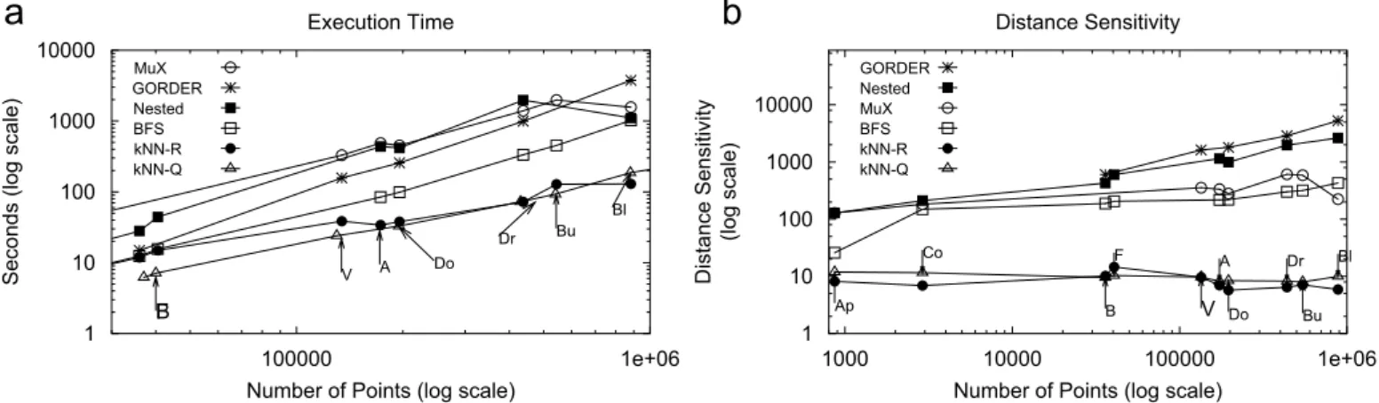
We evaluated our algorithm by comparing the execution time and the distance sensitivity of our algorithm with that of theGORDERmethod[18]and the MuX method[21]. We
also compared our algorithm with traditional methods like thenested join[22]and a variant of the BFS algorithm[10]. We use both a bucket PR quadtree [8]and an R-tree [9] variant of thekNNalgorithm in our study. Our evaluation was in terms of three-dimensional point models as we are primarily interested in databases for computer graphics
applications. The applicability of our algorithm to data of even higher dimensionality is a subject for future research. We first discuss the effect of each of the following three variables on the performance of the algorithms.
(i) The size of the disk pages which is related to the value of the bucket capacity in the construction of the bucket PR quadtree (Section 6.1).
(ii) The memory cache size (Section 6.2).
(iii) The effect of the size of the data set (Section 6.3).
Once we have determined the effect of these variables on the algorithm, we choose appropriate values to compare our algorithm with the other methods in Section 6.4.
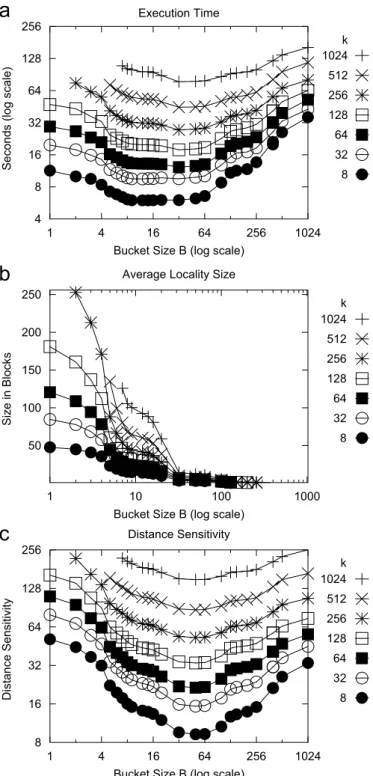
6.1. Effect of bucket capacity (B)
In this section, we study the effect of the bucket capacity Bon the performance of our kNNalgorithm. The bucket capacityBalso corresponds to the size of thedisk page. For a given value ofkbetween 8 and 1024, the value ofBwas varied between 1 and 1024. The performance of our algorithm using a bucket PR quadtree was evaluated by measuring the execution time of the algorithm, the average number of blocks in the locality of the leaf blocks, and the resultingdistance sensitivityof the algorithm. In this set of experiments, we made use of the Stanford Bunny model containing 35,947 points.
Fig. 7a shows the effect ofBon the execution time of the kNNalgorithm. Note that for smaller values ofB ðp16Þ, the kNNalgorithm has a large execution time. However, it quickly decreases for slightly larger values of B . For values of B between 32 and 128, our kNNalgorithm has some of the lowest execution times. Fig. 7b shows the average number of blocks in the locality of the leaf blocks of the bucket PR quadtree. When B is small, the size of the locality is large. As a result, for small values of B the algorithm has a higher execution time. How-ever, as the value of B increases the size of the locality quickly reduces to a small constant value. For larger values of B , the increase in execution time can be attributed to a larger number of points stored in the blocks in the locality, even though the number of blocks in the locality remains almost the same. The sensitivity analysis shown in Fig. 7c is similar to Fig. 7a. To summarize, the kNNalgorithm performs well for moder-ately small values ofB, and in particular for the range ofB between 32 and 128.
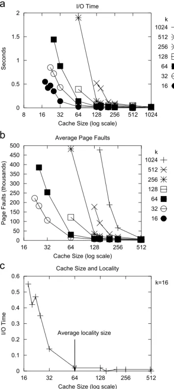
6.2. Effect of cache size
The next set of experiments examines the effect of the cache sizeon the performance of ourkNNalgorithm. The cache size is defined in terms of the number of leaf blocks that can be stored in the main memory. We use a least recently used(LRU)replacement policy on the disk pages stored in the cache. The size of each memory page is
determined by the value ofB. We record the effect of the size of the cache on the resulting number of page faults, and the time spent onI=Ooperations.Figs. 8a–b shows the result of the experiments forB¼32 and for varying values ofkranging between 8 and 1024. We observed high values for the I=Otime and the number of page-faults for small (p32) cache sizes, but these values quickly decreased when the cache size was increased beyond a certain value. This
50 100 150 200 250 1 10 100 1000 Size in Blocks
Bucket Size B (log scale) Average Locality Size
k 1024 512 256 128 64 32 8 8 16 32 64 128 256 1 4 16 64 256 1024 Distance Sensitivity
Bucket Size B (log scale) Distance Sensitivity k 1024 512 256 128 64 32 8 4 8 16 32 64 128 256 1 4 16 64 256 1024
Seconds (log scale)
Bucket Size B (log scale) Execution Time k 1024 512 256 128 64 32 8
Fig. 7. Effect of Bucket capacityBon the: (a) execution time; (b) average size of the locality in blocks, and (c) distance sensitivity for different values ofkfor ourkNNalgorithm.
value, incidentally, corresponds to the average size of the locality, as seen inFig. 8c. Moreover, this also explains the occurrence of large number of page faults when the size of the cache is smaller than the size of the locality. The rule of thumb is that the cache size should be at least as large as the average size of the locality.
6.3. Effect of data set size
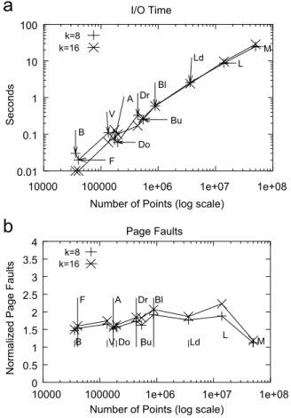
Experiments were also conducted to evaluate the scalability of the algorithm as the size of the input data set is increased. We experimented with several three-dimensional point models ranging in size from 2k to 50 million points as shown inFig. 9. The bucket sizeBand the cache-size were set to 32 points and 500 blocks, respec-tively. The results of the experiments are given in
Figs. 10–11. Fig. 10a shows the effect of size on the time taken to perform thekNNalgorithm.Fig. 10b records the distance sensitivity of the algorithm. As the distance sensitivity of our approach is almost linear, our algorithm exhibits OðnlognÞ behavior. Fig. 10c records the average size of the locality. We also note that the average locality size is almost constant for data sets of all sizes used in the evaluation. Also, the size of the locality showed only a slight increase even as the value ofkis increased from 8 to 16. TheI=Otime and the resultant number of page faults are given inFig. 11.Fig. 11a shows the effect of thesizeof the data set on the time spent by the algorithm on I=O operations. Fig. 11b shows the number of page faults normalized by size for data sets of various sizes. Both the time spent onI=O and the number of page faults exhibit linear dependence on the size of the data set.
6.4. Comparison
We evaluated our algorithm by comparing its execution time and distance sensitivity with that of the GORDER
method[18]and the MuX method of Bo¨hm et al.[19]. Our comparison also includes traditional methods like the nested join [22] and a variant of the BFS algorithm that invoked a BFS algorithm for each point in the data set. We used both a bucket PR quadtree and an R-tree variant of the algorithm in the comparative study. The R-tree implementation of our algorithm used a packed R-tree
[23]with a bucket-capacity of 32 and abranching factorof 8. Note however, that the values of B and k are chosen independent of each other. We retained 10% of the disk pages in the main memory using a LRU based page replacement policy. For theGORDERalgorithm, we used the
parameter values that led to its best performance, accord-ing to its developers [18]. In particular, the size of a sub-segment was chosen to be 1000, the number of grids were set to 100, and the size of the data set buffers was chosen to be more than 10% of the data set size. For the MuX-based method, a page capacity of 100 buckets and a bucket capacity of 1024 points was adopted. There are a few differences between the MuX method as described in[19]
and our implementation. In particular, we adapted our implementation into a three level structure with a set of hosting pages where each page contains several buckets with pointers to a disk-based store. Also, we did not use a fractionatedpriority-queue as described in[19]but replaced it with a heap-based priority queue. However, we did not take into the account the time taken to manipulate the
0 0.5 1 1.5 2 8 16 32 64 128 256 512 1024 Seconds
Cache Size (log scale) I/O Time k 1024 512 256 128 64 32 16 0 50 100 150 200 250 300 350 400 450 500 16 32 64 128 256 512
Page Faults (thousands)
Cache Size (log scale) Average Page Faults
k 1024 512 256 128 64 32 16 0 0.1 0.2 0.3 0.4 0.5 0.6 16 32 64 128 256 512 I/O Time
Cache Size (log scale) Cache Size and Locality
Average locality size
k=16
Fig. 8. Effect of cache size on: (a) the time spent onI=O; (b) the number of page faults; for varying values of k and B¼32; (c) a comparison between the cache size and the average size of the locality fork¼16.
heap structure, thereby ensuring that these differences in the implementation do not affect the comparison results. Also, we only count the point–point distance computations in determining distance-sensitivity and disregard all other distance computations even though they form a substantial fraction of the execution time. We used a bucket capacity of 1024 for the BFS and nested join [22] methods. The results of our experiments were as follows.
(i) Our algorithm clearly out-performs all the other methods for all values of k on the Stanford Bunny model as shown inFig. 12a–b. Our algorithm leads to at least an order of magnitude improvement in the distance sensitivity over the MuX, the GORDER , the
BFS and the nested join techniques for smaller values ofk(p32) and at least 50% improvement for largerk
(o256) as seen inFig. 12b. We observed an improve-ment of at least 50% in the execution time (Fig.12a) over the competing methods.
(ii) However, as size of the input data set is increased the performance of the MuX algorithm was comparable to the nested, BFS and the GORDERbased methods (Fig.
13a). Moreover, our method has an almost constant distance sensitivity even for large data sets. The distance sensitivity of the comparative algorithms are at least an order of magnitude higher for smaller data sets and up to several orders of magnitude higher for the larger datasets in comparison to our method (Fig. 13b). We observed similar execution time speedups as seen inFig. 13a.
(iii) Fig. 13shows similar performance for the R-tree and the quadtree variants of our algorithm.
7. Applications
Having established that our algorithm performed better than theGORDERand MuX methods, we next evaluated the
use of our algorithm in a number of applications for different data sets that included both publicly available and synthetically generated point-cloud models. The size of the models ranged from 35,947 points (Stanford Bunnymodel) to 50 million points (Syn-50 model). These applications include computing the surface normals to each point in the
point-cloud using a variant of the algorithm by Hoppe et al.[2]and removing noise from the point surface using a variant of the bilateral filtering method [3,13]. Fig. 14 shows the time needed for these applications when incorporating an algorithm with a neighborhood of size
k¼8 for each point in the point-cloud model. Fig. 14b shows that our algorithm results in scalable performance even as the size of the data set is increased so that it exceeds the amount of available physical memory in the computer by several orders of magnitude. The scalable nature of our approach is readily apparent from the almost uniform rate of finding the neighborhoods, i.e., 5900 neighborhoods/s for the Stanford Bunny model and 7779 neighborhoods/s for the Syn-50 point-cloud models.
In the rest of this section, we describe in greater detail how our algorithm can be used in these computer graphics applications, and give a qualitative evaluation of its use. In particular, we discuss its use in computing surface normals (Section 7.1), noise removal through mollification of surface normals and bilateral mesh filtering (Section 7.2), as well as briefly mentioning additional related applications (Section 7.3).
7.1. Computing surface normals
Point-cloud models are distinguished from other models by not containing any topological information. Thus, one of the initial preprocessing steps required before the point-cloud model can be successfully used is to compute the surface normal for each point in the model. Computing the surface normal is important for the proper display and rendering of point-cloud data. Using the surface normal information, other topological features of a point surface can be estimated. For example, we can estimate the presence of sharp corners on the point-cloud models with reasonable certainty. A sudden large deviation in the orientation of the surface normals within a small spatial distance may indicate the presence of a sharp corner. Many such local surface properties can be estimated by examin-ing the surface normals and the neighborhood information. One of the most prominent methods for computing surface normals for unorganized points is due to Hoppe et al. [2]. This method relies on computing the kNNs to
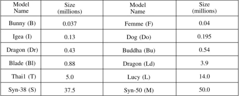
Model Size Model Size Name (millions) Name (millions) Bunny (B) 0.037 Femme (F) 0.04
Igea (I) 0.13 Dog (Do) 0.195 Dragon (Dr) 0.43 Buddha (Bu) 0.54
Blade (Bl) 0.88 Dragon (Ld) 3.9 Thai 1 (T) 5.0 Lucy (L) 14.0 Syn-38 (S) 37.5 Syn-50 (M) 50.0
each point in the data set. The neighborhood isfit with a
hypothetical surface which minimizes the sum of the
squared distances from each point in the neighborhood
to the hypothetical surface. A covariance analysis of the
resulting neighborhood leads to the estimation of the normals to the surface and the query-point.
A more recent contribution is by Mitra et al.[15]which
deals with the computation of the surface normals to a point-cloud in the presence of noise. This algorithm computes the neighborhood of points in the data set after
taking into consideration the sampling density and the curvature of the neighborhood. There is also the alternative
approach of Floater and Reimers[24]thattriangulatesthe
neighborhood and computes the surface normals from the resulting mesh surface.
The neighborhood finding algorithms used in these methods are as diverse as the methods themselves. The
algorithm by Hoppe [2] assumes a uniform sampling of
points in the point-cloud. This makes the computation of neighborhood almost trivial, although not realistic. Also, many algorithms use either an approximate brute-force method or compute the neighborhood by repeated computation of the neighborhood for one point at a time (e.g., see[15]).
We computed the surface normal information of several
data sets using a method similar to that of Hoppe et al.[2].
We tabulated the time taken for data sets of different sizes and also recorded the effect of varying the size of the neighborhood on the resulting neighborhood calculation. The effect of varying the size of the data set when computing the surface normals is given by the
appro-priately labeled column in Fig. 14a. The main results of
using our algorithm to compute surface normals are as follows:
(i) Thequalityof the surface normals depends on the size
of the neighborhood as can be seen inFig. 15. Using
1 10 100 1000 10000
10000 100000 1e+06 1e+07 1e+08
Seconds (log scale)
Number of Points (log scale) Execution Time B F V A Do Dr Bu Bl Ld T L M k=16 k=8 1 10 100
10000 100000 1e+06 1e+07 1e+08
Distance Sensitivity (log scale)
Number of Points (log scale) Distance Sensitivity B F V A Do Dr Bu Bl Ld L M k=8 k=16 100
10000 100000 1e+06 1e+07 1e+08
Size in Blocks (log scale)
Number of Points (log scale) Average Locality Size
B F V A Do Dr Bu Bl Ld L M k=8 k=16
c
Fig. 10. Effect of the size of the data set on: (a) execution time; (b) distance sensitivity, and (c) average locality size for various point models withB¼32 and 500 blocks in the memory cache.
0 0.5 1 1.5 2 2.5 3 3.5 4
10000 100000 1e+06 1e+07 1e+08
Normalized Page Faults
Number of Points (log scale) Page Faults F V A Do Dr Bu Bl Ld L M k=8 k=16 B 0.01 0.1 1 10 100
10000 100000 1e+06 1e+07 1e+08
Seconds
Number of Points (log scale) I/O Time B F V A Do Dr Bu Bl Ld L M k=8 k=16
Fig. 11. Effect of size of the data set on: (a) time spent onI=O; (b) the number of page faults normalized by size for datasets of various sizes.
the surface normals for 8pkp64 retains the finer details on the surface (Figs. 15a–b). Using a larger neighborhood such as kX64 leads to a loss of many of the finer surface details (Fig. 15c). This effect can be attributed to theaveragingproperty of the neighbor-hood.
(ii) When dealing with noisy meshes, the surface normals computed using the topological information of the mesh are often erroneous as can be seen in the dragon model in Fig. 16a. In such cases, we can use our kNNalgorithm to compute the surface normals by just using the neighborhood of the points and the result is relatively error-free as seen in Fig. 16b when using 8 neighbors. This leads us to observe that correct surface normals are important for the proper display of the point model, and that the normals computed by analyzing the neighborhood are resilient to noise, but result in a loss in surface details if an unsuitable value ofkis used as seen inFig. 15c.
7.2. Noise removal
With advances in scanning technologies, many objects are being scan converted into point-clouds. The objects are scanned at a high resolution in order to capture the surface details and to provide an illusion of a smooth compact surface by the close placement of the points comprising the point-cloud model. However, in reality, points in a freshly scanned point-cloud model are noisy due to environmental interference, material properties of the scanned object, and calibration issues with the scanning device. Often, an additional corrective procedure needs to be performed in order to account for the residual noise before the model can be successfully employed. In fact, such an unprocessed point-cloud model would have a scarred appearance as illustrated inFig. 16a which has been obtained by adding a noise element to each of the points in the original model.
Noise is removed by applying a filtering algorithm to the points in the point-cloud model. Bilateral mesh filtering
1 10 100 1 2 4 8 16 32 64 128 256 Seconds k (log scale) Execution Time MuX GORDER Nested BFS kNN-R kNN-Q 0.25 1 4 16 64 256 1024 1 2 4 8 16 32 64 128 256 Distance Sensitivity (log scale) k (log scale) Distance Sensitivity GORDER Nested BFS MuX kNN-R kNN-Q
a
b
Fig. 12. Performance comparison of ourkNNalgorithm with the BFS,GORDER, MuX and the Nested join algorithms. ‘kNN-Q’ and ‘kNN-R’ refers to the quadtree and R-tree implementations of our algorithm respectively. Plots a–b show the performance of the techniques on theStanford Bunnymodel containing 35,947 points for values ofkranging between 1 and 256; (a) execution time, and (b) distance sensitivity.
1 10 100 1000 10000 100000 1e+06
Seconds (log scale)
Number of Points (log scale) Execution Time B F V A Do Dr Bu Bl MuX GORDER Nested BFS kNN-R kNN-Q 1 10 100 1000 10000 1000 10000 100000 1e+06 Distance Sensitivity (log scale)
Number of Points (log scale) Distance Sensitivity Ap Co B F V A Do Dr Bu Bl GORDER Nested MuX BFS kNN-R kNN-Q
a
b
Fig. 13. Performance comparison of ourkNNalgorithm with the BFS,GORDER, MuX and the Nested join algorithms. ‘kNN-Q’ and ‘kNN-R’ refers to the quadtree and R-tree implementations of our algorithm, respectively. Plots a–b record the performance of all the techniques on data sets of various sizes for
[3,13]and mollification[25] are two prominent techniques for removing noise from a mesh. While the bilateral mesh filtering algorithm attempts to correct the position of erroneous points, the mollification approach, instead, tries to correct the surface normals at the point. Bilateral mesh
filtering is analogous to displacement mapping [26] and
mollification is analogous to bump mapping [27], both of
which are prominent texturing techniques that can be used to achieve the same result. In particular, displacement mapping relies on shifting the points themselves to bring about texturing of the surface, while bump-mapping modifies the surface normals at each vertex of the mesh surface. Bilateral filtering differs from another class of
techniques, that include MLS noise removal [28], which
Model Name Size (millions) kNN Surface Normals Noise Removal Bunny (Bu) 0.037 6.22 9.0 9.64 Femme (F) 0.04 7.13 10.5 13.9 Igea (I) 0.13 24.05 36.6 47.52 Dog (Do) 0.195 32.9 53.4 64.45 Dragon (Dr) 0.43 72.62 118.9 122.2 Buddha (Bu) 0.54 93.04 152.3 157.25 Blade (Bl) 0.88 185.92 304.2 270.0 Dragon (Ld) 3.9 663.84 900.0 1209.8 Thai (T) 5.0 940.04 1240.0 1215.7 Lucy (L) 14.0 2657.9 3504.0 3877.78 Syn-38 (S) 37.5 4741.79 - -Syn-50 (M) 50.0 6427.5 - -1 10 100 1000 10000
10000 100000 1e+06 1e+07 1e+08
Seconds (log scale)
Number of Points (log scale) Execution Time B F V A Do Dr B u B l Ld T L SM NOISE NORMALS kNN
a
b
Fig. 14. (a) Tabular and (b) graphical views of the execution time of thekNNalgorithm for different point models, and the time to execute a number of operations (i.e., normal computation and noise removal) using it. All results are fork¼8.
correct the points by reconstructing a smooth local surface and re-sampling points from the surface. In the rest of this section, we discuss the results of our application of both bilateral mesh filtering and mollification to remove noise in large point-cloud models.
We applied the bilateral mesh filtering algorithm in[3,13] to the point-cloud model as follows. We initially computed a neighborhood for each point in the model. Our adaptation of the bilateral filtering method assigns weights (an influence measure analogous to the Gaussian weights in the bilateral filtering method) to each point in the neighborhood in such a way that the computation becomes less sensitive to outlier points. Note that mollification corrects the normals instead of the point, but is similar in approach.Fig. 17shows the results of applying our point-cloud model adaptation of the conventional bilateral mesh filtering algorithm to the bunny model (35,947 points) for different pairs of values of the Gaussian kernel. Note that the quality of the results when using our adaptation does not depend on the values of the Gaussian kernel.
As pointed out earlier, mollification is similar to bilateral mesh filtering with the difference being that instead of performing the filtering operation on the points, the filtering operation is applied to the original surface normals of the points. In order to evaluate the sensitivity of our filtering and surface computation methods to noise, we added Gaussian noise using the Box–Muller method[29]to a bunny mesh-model. We computed the surface normals at
each vertex in the noisy mesh using the connectivity information contained in the mesh. The resultant mesh, disregarding the connectivity information, is a point-cloud (as shown inFig. 19a) with noisy point positions and noise-corrupted normals. We use this approach to create the noisy point-clouds used in Figs. 18 and 19. Figs. 19b–d compare the result of using the mollification method (Fig. 19d) with the computation of surface normals as in Section 5.1 (Fig. 19b) and our adaptation of the bilateral mesh filtering method (Fig. 9c). All three methods were applied for 8 neighbors. From the figure, we see that when using ourkNNmethod to compute the neighborhoods to be used in computing the surface normals, there is no perceptible difference between the three methods even in the case of noisy data.
7.3. Related applications
The most obvious application of thekNNalgorithm is in the construction of kNNgraphs [30]. kNNgraphs are useful when repeated nearest neighbor queries need to be performed on a data set. ThekNNalgorithm may also be used in point reaction-diffusion [31] algorithms. Such algorithms mimic a physical phenomenon to uniformly distribute points on a given surface or space. Many of natural texture patterns encountered in nature can be recreated using this technique. The algorithm works as follows. Each point is assigned a unit positive charge. The resultant repulsion force acting on the point is computed using the kNNs at each point. Next, the point is moved along the direction of the force, and the kNNalgorithm is repeatedly reinvoked at each iteration until an equilibrium condition is reached.
A recent contribution in the construction of approximate surfaces from point sets is the moving least squares (MLS) [28] method. Weyrich et al. [14] have identified useful point-cloud operations that use the MLS method. Of these operations, we believe that MLS point-relaxation, MLS smoothing, MLS basedupscaling[28], anddownscalingcan all benefit when used in conjunction with the kNN algo-rithm.
Tools that perform upscaling [32,33] and downscaling [28]of point-clouds all use the kNNalgorithm to generate Fig. 17. Results of applying the neighborhood-based adaptation of the
bilateral mesh filtering algorithm to the bunny model for Gaussian kernel pairs: (a)sf¼2,sg¼0:2; (b)sf¼4,sg¼4, and (c)sf ¼10,sg¼10 for a neighborhood of size 8. The results are independent of the size of the Gaussian kernel that was chosen.
Fig. 16. (a) A noisy mesh-model of a dragon, and (b) the corresponding model whose surface normals were recomputed using ourkNNalgorithm. The algorithm took about 118 seconds and used eight neighbors.
varied levels of detail (LOD) [34] of point models. The
quadratic error simplification method [32,33] simplifies a point-cloud by removing the points that make the least significant contribution to the surface details. We have built a sample tool that implements Garland’s method[32]
on point-clouds and have used it to generate Igea point models of different sampling-rate of as seen inFig. 20. The Igea model of size 135k was reduced to smaller models of sizes 14k, 48k, 78k, 99k and 111k, the largest of which took less than 120 seconds to generate. The general quality of the reduced model produced by the tool however depends on the extent by which the models were reduced. For example, we can note some loss in facial features in Fig. 20 (14k) while Fig. 20 (111k) is almost identical to the original model.
A similar method to increase the point sampling uses a variant of MLS [28] to insert additional points in the neighborhood (termedupscaling). The algorithm computes
theknearest neighbors to each point using thekNN algo-rithm. Points are then evenly distributed [35] on the hypothetical surface that is fit through the points in the neighborhood. We built a variant of the algorithm which when applied to theapplemodel (Fig.21a) containing 867 points resulted in a new point model containing 27,547 points (Fig.21b) which took about 1.2 s to construct.
8. Concluding remarks
We have presented a new kNNalgorithm that yields an improvement of several orders of magnitude for distance sensitivity and at least one order of magnitude improve-ment in execution time over an existing method known as GORDER designed for dealing with large volumes of data that are disk-resident. We have applied our method to point-clouds of varying size including some as large as 50 million points with good performance. A number of Fig. 19. (a) A bunny point-cloud model to which Gaussian noise was added, and the result of applying; (b) the surface normal computation method in Section 5.1; (c) our adaptation of bilateral mesh filtering, and (d) mollification.
Fig. 18. Three noisy models which were de-noised using filtering and mollification techniques. In the pairs of figures shown for each of the models, the figure on the left is the noisy model, while the figure on the right is the corrected point model. The (a)Igeaand (b)dogmodels were denoised with the filtering method, while the (c)femmemodel was denoised using the mollification technique.
applications of the algorithm were presented. Below, we summarize a few interesting directions for future research. (i) Although our focus was on the computation of the exactkNNs, our methods can also be applied to work with approximatekNNs by simply stopping the search for the kNNs when k neighbors of the query point withinof the true distance of thekth neighbor have been found. An interesting problem is to devise an
approximate locality L of a block b, such that L contains the -approximate kNNs of all the points contained inb.
(ii) We have shown that for a given subdivision of space, the BUILDLOCALITYalgorithm isoptimal, although, the
time taken to perform the algorithm depends solely on our choice of the data structure. It is not difficult to see that certain point data set and data structure config-urations may result in large localities of the points. An interesting direction of research is the design and analysis of a data structure that can ensure that the average size of the locality is small, thereby providing good performance.
(iii) Our kNNalgorithm only requires the ability to compute MinDist, MaxDist, and the number of points contained in a block. An interesting study would be to examine if smaller localities can be built if additional statistics on the distribution of the points contained in a block, such as the MAXNEARESTDIST
estimator[8], were available to the algorithm.
(iv) Modify our kNNalgorithm to provide k nearest neighbors that are radially well distributed around the query point. It is not clear if a localityLof a block bcan be defined, such that all the radial neighbors of all the points inb are contained inL.
(v) Explore the applicability of some of the concepts discussed here to high-dimensional datasets using techniques such as those described in[36,18].
Acknowledgments
The authors would like to gratefully acknowledge the support of the National Science Foundation under Grants CCF-0515241 and EIA-00-91474, Microsoft Research, and the University of Maryland General Research Board. The authors would like to thank the anonymous reviewers for their useful comments and suggestions which helped improve the quality of this paper immensely. Special thanks are due to Chenyi Xia for providing us with the
GORDER source code. The point models used in the paper
are the creations of the following individuals or institu-tions. The Bunny, Buddha, Thai, Lucy and the Dragon models are from the Stanford 3D Scanning Repository. TheIgeaand theDinosaurmodels are from Cyberware Inc. TheTurbine blademodel was obtained from the CD-ROM associated with the Visualization Toolkit [37] book. The Dog model is from MRL-NYU. The Femme model is thanks to Jean-Yves Bouguet.
References
[1] Andersson M, Giesen J, Pauly M, Speckmann B. Bounds on the
k-neighborhood for locally uniformly sampled surfaces. In: Proceed-ings of the eurographics symposium on point-based graphics, Zurich, Switzerland; 2004. p. 167–71.
[2] Hoppe H, DeRose T, Duchamp T, McDonald J, Stuetzle W. Surface reconstruction from unorganized points. In: Proceedings of the SIGGRAPH’92 conference. Chicago, IL: ACM Press; 1992. p. 71–8. [3] Jones TR, Durand F, Desbrun M. Noniterative, feature-preserving mesh smoothing. In: Proceedings of the SIGGRAPH’03 conference, vol. 22(3). San Diego, CA: ACM Press; 2003. p. 943–49.
[4] Levoy M, Pulli K, Curless B, Rusinkiewicz S, Koller D, Pereira L, Ginzton M, Anderson S, Davis J, Ginsberg J, Shade J, Fulk D. The digital Michelangelo project: 3D scanning of large statues. In: Proceedings of the SIGGRAPH’00 conference, New Orleans, LA: ACM Press; 2000. p. 131–44.
[5] Pauly M, Keiser R, Kobbelt LP, Gross M. Shape modeling with point-sampled geometry. ACM Trans. Graph. 2003;22(3): 641–50.
[6] Clarkson KL. Fast algorithm for the all nearest neighbors problem. In: Proceedings of the 24th IEEE annual symposium on foundations of computer science, Tucson, AZ, 1983, p. 226–32.
Fig. 20. Sizes and execution times for the result of applying a variant of the simplification algorithm[32]using thekNNalgorithm to theIgeapoint model of size 135k.
Fig. 21. (a) Initial apple model (867 points) and (b) the result of applying an upscaling algorithm to it using thekNNalgorithm (27,547 points).