Accelerating Pathology Image Data Cross-Comparison on
CPU-GPU Hybrid Systems
Kaibo Wang
1Yin Huai
1Rubao Lee
1Fusheng Wang
2,3Xiaodong Zhang
1Joel H. Saltz
2,3 1Department of Computer Science and Engineering, The Ohio State University
2
Center for Comprehensive Informatics, Emory University
3Department of Biomedical Informatics, Emory University
1{
wangka,huai,liru,zhang
}@cse.ohio-state.edu
2,3{fusheng.wang,jhsaltz
}@emory.edu
ABSTRACT
As an important application of spatial databases in pathol-ogy imaging analysis, cross-comparing the spatial bound-aries of a huge amount of segmented micro-anatomic ob-jects demands extremely data- and compute-intensive op-erations, requiring high throughput at an affordable cost. However, the performance of spatial database systems has not been satisfactory since their implementations of spatial operations cannot fully utilize the power of modern parallel hardware. In this paper, we provide a customized software solution that exploits GPUs and multi-core CPUs to acceler-ate spatial cross-comparison in a cost-effective way. Our so-lution consists of an efficient GPU algorithm and a pipelined system framework with task migration support. Extensive experiments with real-world data sets demonstrate the ef-fectiveness of our solution, which improves the performance of spatial cross-comparison by over 18 times compared with a parallelized spatial database approach.
1.
INTRODUCTION
Digitized pathology images generated by high resolution scanners enable the microscopic examination of tissue spec-imens to support clinical diagnosis and biomedical research [10]. With the emerging pathology imaging technology, it is essential to develop and evaluate high quality image anal-ysis algorithms, with iterative efforts on algorithm valida-tion, consolidavalida-tion, and parameter sensitivity studies. One essential task to support such work is to provide efficient tools for cross-comparing millions of spatial boundaries of segmented micro-anatomic objects. A commonly adopted cross-comparing metric is Jaccard similarity [35], which com-putes the ratio of the total area of the intersection divided by the total area of the union between two polygon sets.
Building high-performance cross-comparing tools is chal-lenging, due to data explosion in pathology imaging anal-ysis, as in other scientific domains [22, 27]. Whole-slide
images made by scanning microscope slides at diagnostic resolution are very large: a typical image may contain over 100,000x100,000 pixels, and millions of objects such as cells or nuclei. A study may involve hundreds of images obtained from a large cohort of subjects. For a large-scale interrelated analysis, there may be dozens of algorithms — with vary-ing parameters — generatvary-ing many different result sets to be compared and consolidated. Thus, derived data from images of a single study is often in the scale of tens of terabytes, and will be increasingly larger in future clinical environments.
Pathologists mainly rely on spatial database management systems (SDBMS) to execute spatial cross-comparison [36]. However, cross-comparing a huge amount of polygons is time-consuming using SDBMSs, which cannot fully utilize the rich parallel resources of modern hardware. In the era of high-throughput computing, unprecedentedly rich and low-cost parallel computing resources, including GPUs and multi-core CPUs, have been available. In order to use these resources for maximizing execution performance, applica-tions must fully exploit both thread-level and data-level par-allelisms and well utilize SIMD (Single Instruction Multiple Data) vector units to parallelize workloads.
However, supporting spatial cross-comparison on a CPU-GPU hybrid platform imposes two major challenges. First, parallelizing spatial operations, such as computing areas of polygon intersection and union, on GPUs requires efficient algorithms. Existing CPU algorithms, e.g., those used in SDBMSs, are branch intensive with irregular data access patterns, which makes them very hard, if not impossible, to parallelize on GPUs. Efficient GPU algorithms, if exist, must successfully exploit massive data parallelisms in the cross-comparing workload and execute them in an SIMD fashion. Second, a GPU-friendly system framework is re-quired to drive the whole spatial cross-comparing workload. The special characteristics of the GPU device require data batching to mitigate communication overhead, and coordi-nated device sharing to control resource contention. Fur-thermore, due to the diversity of hardware configurations and workloads, task executions have to be balanced between GPUs and CPUs to maximize resource utilization.
In this paper, we present a customized solution, SCCG (Spatial Cross-comparison on CPUs and GPUs), to address the challenges. Through detailed profiling, we identify that the bottleneck of cross-comparing query execution mainly comes from computing the areas of polygon intersection and union. This explains the low performance of SDBMSs and
Permission to make digital or hard copies of all or part of this work for personal or classroom use is granted without fee provided that copies are not made or distributed for profit or commercial advantage and that copies bear this notice and the full citation on the first page. To copy otherwise, to republish, to post on servers or to redistribute to lists, requires prior specific permission and/or a fee. Articles from this volume were invited to present their results at The 38th International Conference on Very Large Data Bases, August 27th - 31st 2012, Istanbul, Turkey.
Proceedings of the VLDB Endowment,Vol. 5, No. 11
motivates us to design an efficient GPU algorithm, called PixelBox, to accelerate the spatial operations. Both the design and the implementation of the algorithm are opti-mized thoroughly to ensure its high performance on GPUs. Moreover, we develop a pipelined system framework for the whole workload, and design a dynamic task migration com-ponent to solve the load balancing problem. The pipelined framework has advantages for its natural support of data batching and GPU sharing. The task migration component further improves system throughput by balancing workloads between GPUs and CPUs.
The main contributions of this paper are as follows: 1) PixelBox, an efficient GPU algorithm and its optimized im-plementation for computing Jaccard similarity of polygon sets; 2) a pipelined framework with task migration support for spatial cross-comparison on a CPU-GPU hybrid plat-form; and 3) a demonstration of our solution’s performance (18x speedup over a parallelized SDBMS) with extensive and intensive experiments using real-world pathology data sets.
The rest of the paper is organized as follows. Section 2 introduces the background and identifies the problem with SDBMSs in processing spatial cross-comparing queries. Our GPU algorithm, PixelBox, is presented in Section 3 to accel-erate the bottleneck spatial operations. Section 4 introduces the pipelined framework and the design of a task migration facility for workload balancing. Comprehensive experiments and performance evaluation are presented in Section 5, fol-lowed by related works in Section 6 and conclusions in Sec-tion 7.
2.
PROBLEM IDENTIFICATION
2.1
Background: Spatial Cross-Comparison
A critical step in pathology imaging analysis is to extract the spatial locations and boundaries of micro-anatomic ob-jects, represented with polygons, from digital slide images using segmentation algorithms [10]. The effectiveness of a segmentation algorithm depends on many factors, such as the quality of microtome staining machines, staining tech-niques, peculiarities of tissue structures and others. A slight change of algorithm parameters may also lead to dramatic variations in segmentation output. As a result, evaluating the effectiveness and sensitivity of segmentation algorithms has been very important in pathology imaging studies.
The core operation is to cross-compare two sets of poly-gons, which are segmented by different algorithms or the same algorithm with different parameters, to obtain their degree of similarity. Jaccard similarity, due to its simplicity and meaningful geometric interpretation, has been widely used in pathology to measure the similarity of polygon sets. SupposeP and Q are two sets of polygons representing the spatial boundaries of objects generated by two methods from the same image. Their Jaccard similarity is defined as
J=kP∩Qk
kP∪Qk,
where P ∩Q and P ∪Q denote the intersection and the union ofP andQ, andk · kis defined as the area of one or multiple polygons in a polygon set. To further simplify the computation, researchers in digital pathology use a variant
definition of Jaccard similarity: let r(p, q) =kkpp∩∪qqkk, then
J′=h{r(p, q) :p∈P, q∈Q,kp∩qk 6= 0}i, (1) in whichh·irepresents the average value of all the elements in a set. The greater the value of J′ is, the more likelyP
andQresemble each other. Compared withJ,J′ does not consider missing polygons that appear in one polygon set but have no intersecting counterpart in the other. Missing polygons can be easily identified by comparing the number of polygons that appear in the intersection with the number of polygons in each polygon set. Other additional measure-ments of similarity, such as distance of centroids, are omitted in our discussion, as their computational complexity is low. What makes the computation of J′ highly challenging
is the huge amount of polygons involved in spatial cross-comparison. Due to the high dependability required by med-ical analysis, the image base has to be sufficiently large — hundreds of whole slide images are common, with each im-age generating millions of polygons. Since a single imim-age contains a great number of objects, the average size of poly-gons extracted from pathology images is usually very small. To expedite both segmentation and cross-comparing, large image files are usually pre-partitioned into many small tiles so that they can fit into memory and allow parallel segmen-tations. The generated polygon files for each whole image also reflect the structure of such partitioning: polygons ex-tracted from a single tile are contained in a single polygon file; a group of polygon files constitute the segmentation re-sult for a whole image; different segmentation rere-sults for the same image are represented with different groups of polygon files, which are cross-compared with each other for the pur-pose of algorithm validation or sensitivity studies.
In the rest of the paper, we refer to the area of the inter-section of two polygons asarea of intersection, and the area of the union of two polygons asarea of union.
2.2
Existing Solutions with SDBMSs
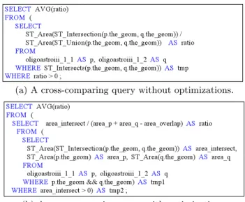
Pathologists mainly rely on SDBMSs to support spatial cross-comparison [36]. In this solution, the cross-comparing workflow typically consists of three major steps: first, poly-gon files (raw data) are loaded into the database; second, indexes are built based on the minimum bounding rectan-gles (MBRs) of polygons; finally, queries are executed to compute the similarity score. Figure 1(a) shows a cross-comparing query in PostGIS [1] SQL grammar that com-putes the Jaccard similarity of two polygon sets, named ‘oligoastroiii 1 1’ and ‘oligoastroiii 1 2’. The join condition is expressed with spatial predicateST Intersects, which tests whether two polygons have intersection. For each pair of in-tersecting polygons, their area of intersection, area of union, and thus the ratio of the two areas are computed. Spa-tial operators ST Intersection and ST Union compute the boundaries of the intersection and the union of two poly-gons, while ST Area returns the area of one or a group of polygons. Finally, these ratios are averaged to derive the similarity score for the whole image.
According to the formulakp∪qk=kpk+kqk − kp∩qk, the query can be re-written so that only theST Intersection
operator is executed for each pair of intersecting polygons, while the area of union can be computed indirectly through the formula. Moreover, ST Intersectscan also be removed since we only need records withratio >0 and whether two
(a) A cross-comparing query without optimizations.
(b) A cross-comparing query with optimizations.
Figure 1: Cross-comparing queries for the Jaccard similarity of
two polygon sets extracted from the same image.
polygons intersect can be determined by their area of inter-section. By replacingST Intersectswith the && operator, which tests whether the MBRs of two polygons intersect, we can further optimize the query, as shown in Figure 1(b).
2.3
Performance Profiling of SDBMS Solution
To identify the performance bottleneck of cross-comparing queries in SDBMSs, we performed a set of experiments with PostGIS, a popular open-source SDBMS 1 2. We used a
real-world data set extracted from a brain tumor slide im-age. The total size of the data set in raw text format is about 750MiB, with two sets of polygons (representing tu-mor nuclei) each containing over 450,000 polygons, and over 570,000 pairs of polygons with MBR intersections. Details of the platform and the data set will be described in Section 5. We split the query execution into separate components, and profiled the time spent by the query engine on each component during a single-core execution. The result is pre-sented in Figure 2 for both the unoptimized and optimized queries. Index Search refers to the testing of MBR intersec-tions based on the indexes built. Area Of Intersection and Area Of Union represent computing the areas of intersection and union, which correspond to the two combo operators,
ST Area(ST Intersection())andST Area(ST Union()). ST Area denotes the other two stand-aloneST Area opera-tors in the optimized query.
For the unoptimized query,ST Intersects(21.8%),
Area Of Intersection (37.4%), and Area Of Union (36.7%) take the highest percentages of execution time, represent-ing the bottlenecks of the query execution. For the op-timized query, since ST Intersects and Area Of Union are removed from the SQL statement,Area Of Intersection be-comes the sole performance bottleneck, capturing almost 90% of the total query execution time. As the left two bars show, very little time (less than 6%) was spent on in-dex building and inin-dex search in both queries. The bar for
1
We also performed similar experiments on a mainstream commercial SDBMS, but its performance was much worse. For simplicity, we only present the results with PostGIS.
2
Based on our communication with the community of SciDB [2], spatial cross-comparing queries are not natively sup-ported by SciDB.
Figure 2: Execution time decomposition of cross-comparing
queries in PostGIS on a single core.
ST Area shows that the time to compute polygon areas is negligible, and further indicates that the high overhead of
Area Of IntersectionandArea Of Unioncomes from spatial operatorsST IntersectionandST Union.
The profiling result explains the low performance of spa-tial databases in supporting cross-comparing queries — com-puting the intersection/union of polygons is too costly as the number of polygon pairs is large. SDBMSs usually rely on some geometric computation libraries, e.g., GEOS [3] in PostGIS, to implement spatial operators. Designed to be
general-purpose, the algorithms used by these libraries to compute the intersection and union of polygons are compute-intensive and very difficult to parallelize. We analyzed the source codes of respective functions for computing poly-gon intersection and union in GEOS and another popular geometric library, CGAL [4], and find that only very few sections of codes can be parallelized without significantly changing algorithm structures. Both GEOS and CGAL use generic sweepline algorithms [11], which are not built for computationally intensive queries and thus lead to the lim-ited performance in SDBMSs.
Using a large computing cluster can surely improve system performance. However, unlike in many high-performance computing applications, pathologists can barely afford ex-pensive facilities in real clinical settings [24]. A cost-effective and meanwhile highly productive solution is thus greatly de-sirable. This motivates us to design a customized solution to accelerate large-scale spatial cross-comparisons. To elim-inate the performance bottleneck, our solution needs an effi-cient GPU algorithm for computing the areas of intersection and union, as will be introduced in the next section.
3.
THE PIXELBOX ALGORITHM
We describe a GPU algorithm,PixelBox, that accepts an array of polygon pairs as input and computes their areas of intersection and union. The design of PixelBox mainly solves three problems: 1) how to parallelize the computa-tion of area of interseccomputa-tion and area of union on GPUs, 2) how to reduce compute intensity when polygon pairs are relatively large, and 3) how to implement the algorithm ef-ficiently on GPUs. We use the terms of NVIDIA CUDA [5] in our description. However, the algorithm design is general and applicable to other GPU architectures and program-ming models as well.
3.1
Pixelization of Polygon Pairs
As measured in the previous section, computing the exact boundaries of polygon intersection/union incurs enormous overhead and has been the main cause to the low perfor-mance of SDBMSs in processing cross-comparing queries. However, the most relevant component to the definition of Jaccard similarity (as shown in Formula 1) is the areas, not
Figure 3: Polygons extracted from medical images have axis-aligned edges and integer-valued vertices.
the intermediate boundaries. As a key to enable paralleliza-tion on GPUs, PixelBox directly computes the areas without resorting to the exact forms of the intersections or unions.
Polygons extracted from medical images share a common property:the coordinates of vertices are integer-valued, and the directions of edges are either horizontal or vertical. This kind of polygons are a special form of rectilinear polygons [34]. As illustrated in Figure 3, since medical images are usually raster images, the boundary of a segmented polygon follows the regular grid lines at the pixel granularity.
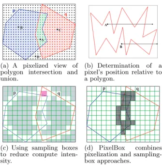
Taking advantage of this property, PixelBox treats a poly-gon as a continuous region surrounded by its spatial bound-ary on a pixel map. As shown in Figure 4(a), pixels within the MBR of polygonsp and q can be classified into three categories: 1) pixels (e.g.,A) lying inside bothpandq, 2) pixels (e.g.,B andC) lying inside one polygon but not the other, and 3) pixels (e.g.,D) lying outside both. The area of intersection (kp∩qk) can be measured by the number of pixels belonging to the first category. The area of union (kp∪qk) corresponds to the number of pixels in the first and second categories. Finally, pixels in the third category do not contribute to eitherkp∩qkorkp∪qk. The pixelized view of polygon intersection and union averts the hassle of com-puting boundaries and, more importantly, exposes a great opportunity for exploiting fine-grained data parallelism hid-den in the cross-comparing computation.
In order to determine a pixel’s position relative to a poly-gon, a well-known method is to cast a ray from the pixel and count its number of intersections with the polygon’s bound-ary [28]. As illustrated in Figure 4(b), if the number is odd, the pixel (e.g., A) lies inside the polygon; if the number is even, the pixel (e.g.,B) lies on the outside.
The pixelization method is very suitable for execution on GPUs. Since testing the position of one pixel is totally inde-pendent of another, we can parallelize the computation by having multiple threads process the pixels in parallel. More-over, since the positions of different pixels are computed against the same pair of polygons, the operations performed by different threads follow the SIMD fashion, which is re-quired by GPUs. Finally, the area of intersection and area of union can be computed altogether during a single traver-sal of all pixels with almost no extra overhead, because the criteria for testing intersection (which uses Boolean AND operation) and union (which uses Boolean OR operation) are both based on each pixel’s positions relative to the same polygon pair. As the number of input polygon pairs is large, we can delegate them to multiple thread blocks. For each polygon pair, the contributions of all pixels in the MBR can be computed by all threads within a thread block in parallel.
3.2
Reduction of Compute Intensity
The pixelization method described above has a weakness — the compute intensity rises quickly as the number of pix-els contained in the MBR increases. Even though polygons
(a) A pixelized view of polygon intersection and union.
(b) Determination of a pixel’s position relative to a polygon.
(c) Using sampling boxes to reduce compute inten-sity.
(d) PixelBox combines pixelization and sampling-box approaches.
Figure 4: The principles of PixelBox.
are usually very small in pathology imaging applications, as the resolution of scanner lens increases, the sizes of polygons may also increase accordingly to capture more details of the objects. There are also cases when the areas of intersection and union are computed between a small group of relatively large polygons and many small polygons, e.g., when pro-cessing an image with a few capillary vessels surrounded by many cells. Moreover, as will be shown in Section 5, even when polygons are small, it is still possible to further bring down the compute intensity and improve performance.
To reduce the intensity of computation and make the al-gorithm more scalable, PixelBox utilizes another technique, calledsampling boxes, whose idea is similar to theadaptive mesh refinement method [9] in numerical analysis. Due to the continuity of the interior of a polygon, the positions of pixels havespatial locality – if one pixel lies inside (or out-side) a polygon, other pixels in its neighborhood are likely to lie on the inside (or outside) too, with exceptions near the polygon’s boundary. Exploiting this property, we can calculate the areas of intersection and union region by re-gion, instead of pixel by pixel, so that the contribution of all pixels in a region may be computed at once.
This technique is illustrated in Figure 4(c). The MBR of a polygon pair is recursively partitioned into sampling boxes, first at coarser granularity (see the large grid cells in the figure), then going finer at selected sub-regions (e.g., as shown by the small boxes near the top) which need fur-ther exploration. For example, when computing the area of intersection, if a sampling box lies completely inside both polygons, the contribution of all pixels within the sampling box is obtained at once, which equals the size of the sam-pling box; otherwise, the samsam-pling box needs to be parti-tioned into smaller sub-sampling boxes and tested further. In Figure 4(c), the grey sampling boxes do not need to be further partitioned because their contributions to the areas of intersection and union are already determined.
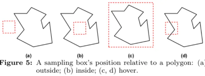
Similar to the pixelization method, the sampling-box ap-proach requires computing a sampling box’s position relative to a polygon, which has three possible values: inside– every pixel in the box lies inside the polygon;outside– every pixel
Figure 5: A sampling box’s position relative to a polygon: (a) outside; (b) inside; (c, d) hover.
in the box lies outside the polygon; andhover– some pixels lie inside while others lie outside the polygon.
Lemma 1. A sampling box’s position relative to a polygon
is determined by three conditions: (i) none of the sampling box’s four edges crosses through the polygon’s boundary; (ii) none of the polygon’s vertices lies inside the sampling box; (iii) sampling box’s geometric center lies inside the polygon. The sampling box lies inside the polygon if all three con-ditions are true; it lies outside the polygon if the first two conditions are true but the last is false; it hovers over the polygon in all other cases, when condition (i) or (ii) is false.
Lemma 1 gives the criteria for computing a sampling box’s position, which is further illustrated in Figure 5. For each sampling box, its four edges are tested against the polygon’s boundary. If there are edge-to-edge crossings, the sampling box must hover over the polygon (case (d) in Figure 5). Otherwise, if any of the polygon’s vertices lies inside the sampling box, the entire polygon must be contained in the sampling box due to the continuity of its boundary, in which case the position is also hover (case (c) in Figure 5); if none of the polygon’s vertices is inside the sampling box, the sam-pling box may be either totally inside (case (b) in Figure 5) or totally outside (case (a) in Figure 5) the polygon , in which case the position of the sampling box’s geometric cen-ter gives the final answer. If the sampling box’s four edges overlap with the polygon’s boundary, the sampling box’s po-sition can be considered as either inside or outside. The next level of partition will distinguish the contribution of each sub-sampling box to the areas of intersection and union.
Testing the position of a sampling box is more costly than doing this for a pixel. When the granularity of a sam-pling box is large, the extra overhead is compensated by the amount of per-pixel computations reduced. However, as sampling boxes are more fine-grained, the cost of computing their positions becomes more significant. Moreover, apply-ing samplapply-ing boxes requires synchronization between coop-erative threads — examination of one sampling box cannot begin until all threads have finished the partitioning of its parent box. Frequent synchronizations lead to low utiliza-tion of computing resources and have been one of the main hazards to performance improvement on GPUs [37].
To retain the merits of both efficient data parallelization and low compute intensity, PixelBox combines pixelization with sampling-box techniques. As depicted in Figure 4(d), sampling boxes are applied at first to quickly finish testing for a large number of regions; when the size of a sampling box becomes smaller than a threshold, T, the pixelization method takes order and finishes the rest of the computation. Unlike the pixelization-only method, computing area of intersection and area of union altogether will incur extra overhead with sampling boxes. For example, if a sampling box hovers over one polygon but lies outside the other, its contribution is clear to the area of intersection, but unclear
to the area of union; in this case, more fine-grained partition-ings are required until the area of union is determined or the pixelization threshold is reached. To reduce the amount of sampling box partitionings and further improve algorithm performance, the area of union is not computed together with the area of intersection in PixelBox. Instead, similar to the query optimization in Figure 1(b), we compute the areas of polygons, and use the formula,kp∪qk=kpk+kqk− kp∩qk, to derive the areas of union indirectly. Computing the area of a simple polygon is very easy to implement on GPUs. With formula3 A = 1
2
Pn−1
i=0(xiyi+1−xi+1yi), in
which (xi, yi) is the coordinate of theith vertex of the poly-gon, we can let different threads compute different vertices and sum up the partial results to get the area.
3.3
Optimized Algorithm Implementation
Algorithm 1 shows the pseudocode of PixelBox. Sampling boxes are created and examined recursively — one region is probed from coarser to finer granularities before the next one. A shared stack is used to store the coordinates of the sampling boxes and the flags showing whether each sam-pling box needs to be further partitioned. For each polygon pair allocated to a thread block, its MBR is pushed onto the stack as the first sampling box (line 13). All threads pop the sampling box on the top of the stack to examine (line 18). If the sampling box does not need to be further probed, all threads will continue to pop the next sampling box (line 19 - 20) until the stack becomes empty and the computation for the polygon pair finishes. For a sampling box that needs to be further examined, if its size is smaller than threshold
T, the pixelization procedure is applied (line 22 - 28); oth-erwise, it is partitioned into sub-sampling boxes, and, after further processing, new sampling boxes will be pushed onto the stack by all threads simultaneously (line 30 - 39).
In the algorithm, PolyAreacomputes the partial area of a polygon handled by a thread; BoxSizereturns the number of pixels contained in a sampling box; PixelInPoly(m, i, p) computes the position of theith pixel in sampling boxm rel-ative to polygonp; SubSampBox(b, i) partitions a sampling boxb and returns theith sub-box for a thread to process; BoxPosition(b, p) computes the position of sampling box
b relative to polygon p; BoxContinuecomputes whether a sampling box needs to be further partitioned based on its positions relative to two polygons; and BoxContribute computes whether a sampling box contributes to the area of intersection according to its position.
The use of a stack to store sampling boxes saves lots of memory space and makes testing sampling box positions and the generation of new sampling boxes parallelized. A synchronization is required before popping a sampling box (line 17) to ensure that thread 0 or the last thread in the thread block has pushed the sampling box to the top of the stack. When threads push new sampling boxes to the stack, they do not overwrite the old stack top (line 37); otherwise, an extra synchronization would be required before pushing new sampling boxes to ensure that the old stack top has been read by all threads. In the current design, the old stack top is marked as ‘no further probing’ (line 38), and will be omitted by all threads when being popped out again.
The GPU kernel only computes the partial areas of inter-sections and the partial summed areas of polygons accumu-lated per thread (lines 5 - 6), which will be reduced later
3
Algorithm 1The PixelBox GPU algorithm. 1: {pi, qi}i: the array of input polygon pairs 2: {mi}i: the MBR of each polygon pair 3: N : total number of polygon pairs
4: stack[] : the shared stack containing sampling boxes 5: I[N][blockDim.x] : partial areas of intersections 6: A[N][blockDim.x] : partial summed areas of polygons 7:
8: procedureKernel SampBox 9: tid←threadIdx.x
10: fori=blockIdx.xtoN do
11: A[i][tid]←A[i][tid] + PolyArea(pi) 12: A[i][tid]←A[i][tid] + PolyArea(qi) 13: Thread 0: stack[0]← {mi,1} 14: top←1
15: whiletop >0do
16: top←top−1 17: syncthreads() 18: {box, c} ←stack[top] 19: if c= 0then
20: continue
21: else
22: if BoxSize(box)< T then
23: forj←tidto BoxSize(box)do
24: φ1←PixelInPoly(box, j, pi)
25: φ2←PixelInPoly(box, j, qi)
26: I[i][tid]←I[i][tid] + (φ1∧φ2)
27: j←j+blockDim.x
28: end for
29: else
30: subbox←SubSampBox(box, tid) 31: φ1←BoxPosition(box, pi) 32: φ2←BoxPosition(box, qi) 33: c←BoxContinue(φ1, φ2) 34: t←BoxContribute(φ1, φ2) 35: a←(1−c)×t×BoxSize(subbox) 36: I[i][tid]←I[i][tid] +a
37: stack[top+ 1 +tid]← {subbox, c}
38: Thread 0: stack[top].c←0 39: top←top+ 1 +blockDim.x
40: end if 41: end if 42: end while 43: i←i+gridDim.x 44: end for 45: end procedure
on the CPU to derive the final areas of intersection and union. Reduction is not performed on the GPU because the number of partial values for each polygon pair is relatively small (equal to the thread block size), which makes it not very efficient to execute on the GPU. We measured the time take by the reductions on a CPU core; the cost is negligible compared to other operations on the GPU.
In the rest of this sub-section, we explain some optimiza-tions employed in the algorithm implementation.
Utilize shared memory. Effectively using shared mem-ory is important for improving program performance on GPUs [32]. The sampling box stack is frequently read and modified by all threads in a thread block, and thus should be allocated in the shared memory. Meanwhile, polygon vertex data are also repeatedly accessed when computing the po-sitions of pixels and sampling boxes. Loading vertices into
shared memory reduces global memory accesses. Due to the limited size of shared memory on GPUs, it is infeasible to al-locate for the largest vertex array size. To make a trade off, we set a static size for the shared memory region containing polygon vertices, and only those polygons whose vertices fit into the region are loaded into the shared memory.
Avoid memory bank conflicts. Bank conflicts happen when threads in a warp try to access different data items re-siding in the same shared memory bank simultaneously. In this case, memory access is serialized which decreases both bandwidth and core utilization. In the sampling box proce-dure, pushing new sampling boxes to the stack may incur bank conflicts if each sampling box is stored continuously in the shared stack. This problem can be solved by separating the stack into five independent ones: four sub-stacks store the coordinates of sampling boxes, and the fifth one stores whether each sampling box needs to be further probed.
Perform loop unrolling. Computing pixel or sampling box positions requires comparing with polygon edges in a loop. Unrolling the loop to have multiple polygon edges tested in a single iteration reduces the number of branch instructions and hides memory latency more efficiently.
3.4
Related Discussions
Pixelization threshold T. The pixelization procedure is applied when the number of pixels contained in a sampling box becomes less than the thresholdT. Let the number of threads in a thread block ben, a good value forT should be betweennandn2. IfT < n, the number of pixels contained
in the last sampling box is less than the number of threads, which will not keep all threads busy during the pixelization procedure; if T > n2, the last sampling box contains too
many pixels, because it could have been further partitioned at least once meanwhile guaranteeing all threads busy during the pixelization procedure. According to our testing (see Section 5.4),T =n2
2 is a very good choice.
Algorithm accuracy. Pixelizing polygons may intro-duce errors into the areas computed. In a general sense, the finer the granularity of pixels is defined, the more accu-rate the computed result is. For pathology imaging analysis, however, PixelBox does not incur any loss of precision. As explained in Section 3.1, the areas computed equal the num-bers of pixels actually lying inside the intersection/union of polygons on the original image. This property generalizes to polygons segmented from any raster image in medical imag-ing and other applications. We validated the correctness of PixelBox by comparing the areas computed by PixelBox with those computed by PostGIS, and find that the results are the same. We regard the generalization of PixelBox to vectorized polygons as a future work.
Implications of PixelBox to other spatial opera-tors. The principal ideas of PixelBox can also be applied to accelerate other compute-intensive spatial operators on GPUs. For example, ST Containscan be implemented by computing the area of intersection and testing whether it equals the area of the object being contained. ST Touches
can be accelerated using ideas similar to PixelBox: compare the edges of one polygon with the edges of the other; also test the positions of vertices in one polygon relative to the other polygon; if there is no edge-to-edge crossing, no vertex of one polygon lies within the other polygon, and at least one vertex of one polygon lies on the edge of the other, these two polygons touches each other; otherwise, they do not touch.
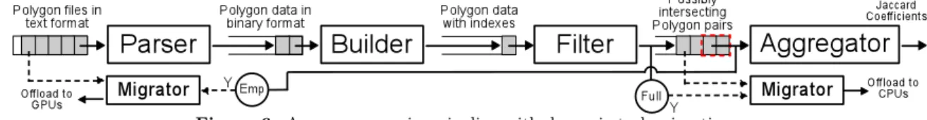
Figure 6: A cross-comparing pipeline with dynamic task migrations.
We believe that many frequently used spatial operators in SDBMSs can be parallelized on GPUs by either directly uti-lizing the PixelBox algorithm or using approaches similar to PixelBox. This is another interesting topic we would like to explore in the future.
4.
SYSTEM FRAMEWORK
Having presented our core GPU algorithm for comput-ing areas of intersection and union, we are now in a posi-tion to introduce how the whole workflow for spatial cross-comparison is implemented and optimized in a CPU-GPU hybrid environment. From the input of the raw text data for polygons to the output of the final results, the workflow con-sists of multiple logical stages. To fully exploit the rich re-sources of the underlying CPU/GPU hardware, these stages must be executed in a controllable and dynamically adapt-able way. To achieve this goal, the system framework must address three challenges: 1) Since GPU has a disconnected memory space from CPU, input data batching for GPU is needed to compensate the long latency of host-device munication; 2) GPU is an exclusive, non-preemptive com-pute device [21], thus uncontrolled kernel invocations may cause resource contention and low execution efficiency on GPU; and 3) task executions have to be balanced between CPUs and GPUs in order to maximize system throughput.
In this section, we present our system framework solu-tion. We first introduce our pipelined structure for the whole workload, and then present our dynamic task migra-tion mechanism between CPUs and GPUs.
4.1
The Pipelined Structure
We have designed and implemented a pipelined structure for the whole workload. Through inter-stage buffers, task productions and consumptions are overlapped to improve resource utilization and system throughput. As depicted in Figure 6, the cross-comparing pipeline comprises four stages: 1. Theparserloads polygon files and transforms the for-mat of polygons from text to binaries. This stage ex-ecutes on CPUs with multiple worker threads. 2. Thebuilderbuilds spatial indexes on the transformed
polygon data. Since polygons are small, Hilbert R-Tree [20] is used to accelerate index building. This stage executes on CPUs in a single thread because its execution speed is already very fast.
3. Thefilterperforms a pairwise index search on the poly-gons parsed from every two polygon files, and gener-ates an array of polygon pairs with intersecting MBRs. Similar to the builder, this stage also executes on CPUs with a single worker thread.
4. Theaggregatorcomputes the areas of intersection and union for each polygon array using our PixelBox al-gorithm. The ratios of areas are then aggregated to derive the Jaccard similarity for a whole image. Poly-gon pairs that do not actually intersect, i.e., with the area of intersection being zero, will not be considered.
A computation task at each pipeline stage is defined at the image tile scale. For example, an input task for the parser is to parse two polygon files segmented from the same image tile; an input task for the builder is to build indexes on the two sets of polygons parsed by a single parser task. In practice, a digital image slide may contain hundreds of small image tiles; each tile may contain thousands of polygons. The granularity of tasks defined at image tile level matches the image segmentation procedure, and allows the workload to propagate through the pipeline in a balanced way.
Utilizing such a pipelined framework is critical to solve the aforementioned challenges. First, the work buffers between pipeline stages provide natural support for GPU input data batching. For example, since the number of polygon pairs filtered may be drastically different from tile to tile, it is nec-essary for the aggregator to group multiple small tasks in its input buffer and send them in a batch to the GPU at once. Second, with a pipelined framework, a single instance of the aggregator consolidates all kernel invocations to the GPUs, which greatly reduces unnecessary contentions and makes the execution more efficient. Finally, the pipelined frame-work creates a convenient environment for load balancing between CPUs and GPUs, as will be introduced next.
4.2
Dynamic Task Migration
Based on the pipelined structure, we have built a task mi-gration component for the whole workflow to achieve load balancing between CPUs and GPUs. First, we have ported the PixelBox algorithms to CPUs (called PixelBox-CPU), and parallelized its execution with multiple worker threads. Second, we have also designed a GPU kernel for the parser stage (called GPU-Parser), whose performance is only com-parable to its CPU counterpart since text parsing requires implementing a finite state machine, which has been shown not very efficient for parallel execution [8]. In this way, the parser and the aggregator stages are flexible to execute tasks on both CPUs and GPUs, which creates an opportunity for balancing workload distributions through dynamic task mi-grations.
What must be noted is that the task migration relies on a special feature of the pipelined framework to detect workload imbalance from the application level. The work buffers between pipeline stages give useful indication on the progress of computation and the status of compute devices. Specifically, if the input buffer of the aggregator stage be-comes full, the migrator knows that this stage is making slow progress and the GPUs have been congested. On the other hand, if the input buffer of the aggregator stage becomes empty, it indicates that the GPUs are being under-utilized. In each case, tasks are dynamically migrated from GPUs to CPUs, or from CPUs to GPUs, to mitigate load imbalance and improve system throughput.
To implement the task migration scheme, two background threads, calledmigration threads, are created — one for the aggregator stage, one for the parser stage. They usually stay in the sleeping state and are only woken up when the input buffer of the aggregator stage becomes full or empty. In the
case of GPU congestion, the aggregator’s migration thread is woken up, which selects the smallest tasks from the in-put buffer of the aggregator and invokes PixelBox-CPU to execute them. In the case of GPU idleness, the parser’s migration thread is woken up to fetch some tasks from the parser’s input buffer and execute them on GPUs. The de-sign of the task migration component is also illustrated in Figure 6.
5.
EXPERIMENTS
This section evaluates our SCCG solution, including the PixelBox algorithm and the system framework. We have im-plemented PixelBox and GPU-Parser with NVIDIA CUDA 4.0. Intel Threading Building Blocks [25], a popular work-stealing software library for task-based parallelization on CPUs, is used to parallelize text parsing and PixelBox-CPU. The pipelined framework is developed using Pthreads. The dynamic task migration component is built into the execu-tion pipeline, and can be turned on or turned off according to the requirements of respective experiments.
5.1
Experiment Methodology
We perform experiments on two platforms. One is a Dell T1500 workstation with an Intel Core i7 860 2.80GHz CPU (4 cores), an NVIDIA GeForce GTX 580 GPU, and 8GiB main memory. The operating system is 64-bit Red Hat En-terprise Linux 6 with 2.6.32 kernel. The other platform is an Amazon EC2 instance with two Intel Xeon X5570 2.93GHz CPUs (totally 8 cores, 16 threads) and two NVIDIA Tesla M2050 GPUs. The size of the main memory is 22 GiB, and the operating system is 64-bit CentOS with 2.6.18 linux ker-nel. T1500 is primarily used to test the performance of the PixelBox algorithm and the pipelined scheme, and to mea-sure the overall performance of SCCG in cross-comparing all data sets. Amazon EC2 instance is used to measure the per-formance of a parallelized PostGIS solution to cross-compare the whole data sets. The task migration component is ver-ified on both platforms. The version of PostGIS we used is 1.5.3; the PostgreSQL version is 9.1.3.
Our experiments use 18 real-world data sets extracted from 18 digital pathology images used in a brain tumor re-search at the authors’ institution. The total size of the data sets in raw text format is about 12GiB. The average size of polygons is about 150 in the number of pixels contained, with the standard deviation around 100. The average num-ber of polygons in each data set is about half million, with the largest data set containing over 2 millions.
In all experiments performed in this paper, we do not consider data loading or disk I/O time for the purpose of fair comparison. First, it is well known that the database system has high loading overhead when processing one-pass data with the “first-load-then-query” data processing model. SCCG averts this problem through customized text parsing and pipelined execution to process the polygon stream on the fly. Second, disk I/O, even though still a significant performance factor for SDBMSs, is not longer the severest bottleneck for cross-comparing queries; most time is spent on computation. The effect of disk I/O can be further miti-gated through SCCG’s pipelined framework by adding a disk pre-fetcher in front of parser stage to sequentially load poly-gon files into main memory. The use of more advanced stor-age devices, such as SSDs and disk arrays, can also reduce
1 10 100 1000
GEOS PixelBox-CPU-S PixelBox
E x e c u ti o n T im e ( s ) 1 10 100 1000 PixelBox-CPU-S PixelBox S p e e d u p
Figure 7: Performance comparison of GEOS and PixelBox.
disk I/O time significantly. Thus, in the following experi-ments, we assume that the polygon data are already loaded into main memory or imported into the database before the pipeline or queries are executed.
5.2
Performance of the PixelBox Algorithm
In this subsection, we evaluate the performance of Pixel-Box and verify some design decisions discussed earlier. The experiments are carried out on the T1500 workstation. Since PostGIS uses GEOS as its geometric computation library, we use the performance of GEOS on a singe core as the baseline in respective experiments. Optimizations similar to the query in Figure 1(b) is used in the baseline to avoid the heavy function call for polygon unions. We select a represen-tative data set, called oligoastroIII 1, for the experiments. It contains 462016 polygons in one polygon set and 458878 polygons in the other. Totally, 619609 pairs of polygons, whose MBRs intersect, are filtered.
In Figure 7, we first show the overall performance of GEOS, PixelBox-CPU on a single core (denoted PixelBox-CPU-S), and PixelBox in computing the areas of intersection and union for all 619609 polygon pairs. Both absolute execu-tion times and relative speedups are shown in logarithmic scales. The computation with GEOS takes over 430 seconds. PixelBox-CPU-S performs better than GEOS thanks to al-gorithm improvement, reducing computation time to about 290 seconds. Compared with GEOS, PixelBox achieves over two-orders-of-magnitude speedup, finishing all computations within only 3.6 seconds. This experiment shows the effi-ciency of PixelBox algorithm that can fully utilize the power of GPUs to accelerate the computation.
In order to validate several algorithm design decisions, i.e., using sampling boxes to reduce compute intensity, and com-puting areas of union indirectly, we do a stress testing with PixelBox using a set of 15724 polygon pairs filtered from two representative polygon files in oligoastroIII 1. We increase the polygon sizes by multiplying the coordinates of polygon vertices with a scale factor whose value varies from 1 to 5. The data sets used in this paper are extracted from slide images captured under 20x objective lens. Considering that the resolution of objective lens commonly used is around 40x at the maximum (which increases the sizes of polygons by 4 times), scaling up the coordinates of polygons by a max-imum factor of 5 (which increases the sizes of polygons by 25 times) is more than sufficient.
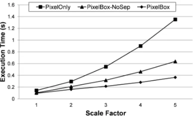
We compare the performance of PixelBox with two base versions: one that uses only the pixelization method (called PixelOnly), the other that combines the pixelization and sampling-box techniques but computes both area of inter-section and area of union directly (called PixelBox-NoSep). We tune the grid size, block size, andT(for PixelBox-NoSep and PixelBox), so that all algorithms execute in their best performance. Their execution times are shown in Figure 8.
Figure 8: Performance of two algorithm decisions: using sam-pling boxes and computing areas of union indirectly.
consistently higher than that of PixelOnly due to the use of sampling boxes, while PixelBox beats the performance of PixelBox-NoSep by further reducing the amount of sam-pling box partitionings performed. When the scale factor is 1, the overhead of per-pixel examination is relatively low be-cause the sizes of polygons are small. But PixelBox-NoSep and PixelBox still out-perform PixelOnly in this case, re-ducing execution time by 28% and 34% respectively. As the scale factor increases, the performance of PixelOnly drops rapidly due to the dramatic increase of the number of pixels that must be handled by the algorithm. However, the per-formance of PixelBox-NoSep and PixelBox only degrades slightly. As the scale factor reaches 5, that is when the sizes of polygons are increased by 25 times, PixelBox-NoSep im-proves over PixelOnly by reducing execution time by over 50%, while PixelBox shortens the execution time even fur-ther by 73% compared with PixelBox-NoSep. This exper-iment verifies the effectiveness of using sampling boxes to reduce compute intensity. It also shows that, by comput-ing areas of union indirectly, the performance of the algo-rithm can be further enhanced due to reduced sampling box partitions. It has to be noted that the performance of Pix-elOnly, PixelBox-NoSep and PixelBox are much higher than the GEOS baseline at all scale factors (it takes GEOS over 11 seconds).
5.3
Effectiveness of Optimization Techniques
On the T1500 workstation, we evaluate the effectiveness of various optimization techniques employed during algorithm implementation, i.e., using shared memory (for loading the polygon vertex data), avoiding bank conflicts (when pushing new sampling boxes), and loop unrolling (when computing positions). We take the same set of 15724 polygon pairs used in the previous experiment, with the scaling factors being 1, 3, and 5, and measure the execution times of four vari-ants of the PixelBox algorithm: PixelBox-NoOpt denotes the base version in which none of the optimization tech-niques are used; PixelBox-NBC denotes the version when bank conflicts are avoided; PixelBox-NBC-UR denotes the version when bank conflicts are avoided and loop unrolling is performed; finally, PixelBox-NBC-UR-SM denotes the ver-sion when all optimizations are utilized. In all variants, the sampling box stack is always allocated in shared memory, because otherwise a global heap whose size is proportional to the total number of threads in the whole grid has to be allocated, which we consider an unreasonable design scheme. The performance of each variant normalized to PixelBox-NoOpt is shown in Figure 9. It can be seen that the
opti-0 0.2 0.4 0.6 0.8 1 1.2 1.4 SF1 SF3 SF5 S p e e d u p Scale Factor
PixelBox-NoOpt PixelBox-NBC PixelBox-NBC-UR PixelBox-NBC-UR-SM
Figure 9: Performance impact of various optimization
tech-niques in algorithm implementation.
mization techniques discussed above are effective in improv-ing the performance of PixelBox. When the scale factor is 1, the performance is improved by a factor of 1.14 after all optimization techniques are utilized; when the scale factor is 5, the speedup raises to a factor of 1.30. The weights of different optimization techniques to the algorithm perfor-mance are, however, varied. The effects of loop unrolling and using shared memory are more significant than that of avoiding bank conflicts. This is because PixelBox spends more time on computing the positions of pixels and sam-pling boxes than on generating new samsam-pling boxes. Thus, loop unrolling and using shared memory, which improves the efficiency of computing positions, play a larger role in the performance of PixelBox.
5.4
Parameter Sensitivity of PixelBox
In order to test the sensitivity of algorithm performance to the pixelization threshold T, we take the same set of 15724 polygon pairs used above and measure how the ex-ecution time of PixelBox varies as we change the value of
T. We do the experiments on the T1500 workstation. We set the thread block size to 64, and the performance trend in each scale factor (SF1 to SF5) is shown in Figure 10. The result verifies our analysis for choosing the value ofT. The performance of PixelBox is sub-optimal whenT is too small or too large. It performs the best when the value ofT
lies between 512 and 4096, which corresponds to the range fromn2/8 ton2, in all scale factors. We also repeated the
experiment when setting thread block size to other values, and the trend was similar. But when the block size is too large (e.g., >= 256), the overall performance of PixelBox degrades. This is because less thread blocks can run con-currently on a multiprocessor and the sampling box
Scheme PostGIS-S NoPipe-S NoPipe-M Pipelined Speedup 1 37.07 63.64 76.02
Table 1: Performance comparisons between different schemes.
tioning will be less fine-grained when block size is too large. According to our experience, settingnto a small value and the value of the pixelization threshold aroundn2
/2 achieves the highest performance.
5.5
Performance of the Pipelined Framework
We evaluate the performance of the pipelined framework in this subsection. Task migration is disabled to remove its influence on the pipeline’s performance. On the T1500 workstation, we collect the execution times of four schemes that cross-compares the oligoastroIII 1 data set:
• PostGIS-S executes the optimized query shown in Fig-ure 1(b) with PostGIS on a single core;
• NoPipe-S uses a single execution stream that executes a non-pipelined version of the framework in Figure 6, in which the four stages execute sequentially on each pair of input polygon files without pipelining;
• NoPipe-M represents the thread-parallel scheme where multiple execution streams are launched with each one invoking NoPipe-S independently;
• Pipelined is the fully pipelined scheme used in SCCG. The result is shown in Table 1, with speedup numbers normalized against the PostGIS-S baseline. Since the bot-tleneck stage of the pipeline has been accelerated by Pix-elBox on GPUs, NoPipe-S achieves over 37-fold speedup compared with PostGIS-S. NoPipe-M performs better than NoPipe-S (63x speedup over PostGIS-S) because simulta-neously issuing multiple streams improves the utilization of resources. However, due to the serialization caused by uncoordinated use of GPUs on the last stage, the CPU resource cannot be well utilized. We measured the CPU utilization during the execution of NoPipe-M and observed that all CPU cores were only about 50% saturated all the times, which confirmed our analysis. The Pipelined scheme achieves the highest performance, accelerating the speed of cross-comparison by a factor of 76 compared with PostGIS-S. The result justifies the use of the pipelined framework and shows the importance of coordination when using GPUs.
5.6
Effectiveness of Dynamic Task Migration
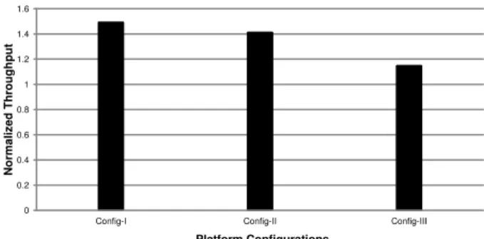
In order to verify the design of the task migration com-ponent, we perform experiments in three different platform configurations: the T1500 workstation (Config-I), the Ama-zon EC2 instance with both GPU cards used (Config-II), and the Amazon EC2 instance with only one GPU card used (Config-III). We use the first two configurations to evaluate the effectiveness of the task migration component to offload workloads from CPUs to GPUs, and use the last one for test-ing load balance in the other direction. Since the GPUs on both platforms are too powerful, in order to make the case of GPU-to-CPU task migrations happen, we purposely slow down PixelBox by selecting a sub-optimal thread block size in Config-III. In real-world system environment, due to con-current sharing of GPUs with other applications, GPUs may not be exclusively occupied by a single application, which is the case we want to emulate in the last configuration.
The oligoastroIII 1 data set is used in experiments. We show the throughput of task-migration-enabled SCCG nor-malized to the throughput of task-migration-disabled SCCG
0 0.2 0.4 0.6 0.8 1 1.2 1.4 1.6
Config-I Config-II Config-III
N o rm a li z e d T h ro u g h p u t Platform Configurations
Figure 11: Performance benefits of dynamic task migration.
in each configuration. Throughput is defined as the size of data set divided by execution time.
As Figure 11 shows, on T1500 workstation, the through-put of SCCG with dynamic task migration is about 50% higher than SCCG without dynamic task migration. In this setting, the aggregator stage cannot keep the GPU fully oc-cupied, which triggers the migrator to dynamically offload tasks from the parser stage to execute on GPU. This im-proves the performance of the parser stage and thus en-hances the throughput. On Amazon EC2 with both GPUs utilized, the GPU resource still cannot be fully utilized by the aggregator stage. Thus, workloads are migrated from CPUs to GPUs, and the throughput of the pipeline is im-proved by over 40%. The throughput improvement is lower than Config-I, because the CPUs are more powerful, which causes less workload offloaded to GPUs. On Amazon EC2 with only one GPU utilized, dynamic task migration im-proves the pipeline throughput by over 14%. In this sce-nario, the aggregator stage becomes the bottleneck of the pipeline, and some aggregator tasks are migrated to execute on CPUs. But due to the relatively small speed gap be-tween the parser and the aggregator stage and the limited performance of PixelBox-CPU on CPUs, the throughput im-provement is smaller compared to other configurations.
5.7
Performance Evaluation with All Data Sets
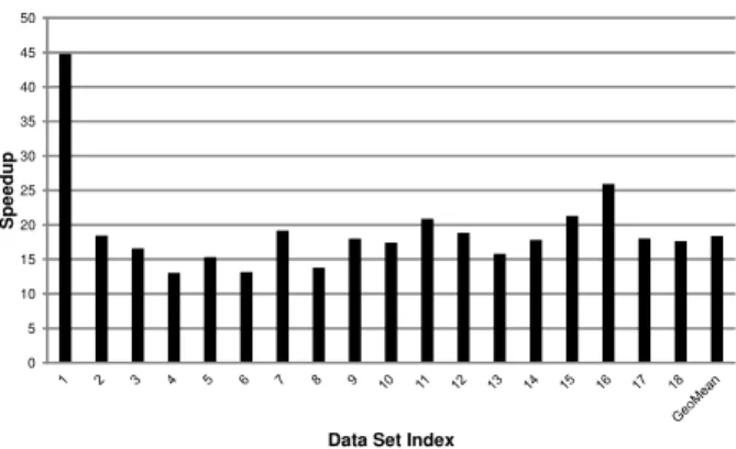
In this section, we give the complete performance results of SCCG compared with a parallelized PostGIS solution over all 18 data sets. The experiments with SCCG are performed on the T1500 workstation with only one GPU card and a 4-core CPU. The experiments with PostGIS are performed on the Amazon EC2 instance with both 4-core CPUs fully utilized. The reason why we choose a less powerful platform for SCCG is to demonstrate both its performance advantage and cost-effectiveness. Query executions in PostGIS are par-allelized over all CPU cores by evenly partitioning polygon tables into 16 chunks and launching 16 query streams to process different chunks concurrently. We refer to this ex-ecution scheme as PostGIS-M. Being generous to PostGIS, we only consider index building and query execution times; time spent on partitioning polygon tables is not included. We measure the times taken by SCCG and PostGIS-M on cross-comparing each data set, and the relative speedups of SCCG compared with PostGIS-M are presented in Fig-ure 12.
To give an impression on the absolute execution times, it takes PostGIS-M over 1120 seconds to process all data sets, while SCCG finishes all computations within only 64 seconds. As Figure 12 shows, the varied speedups of SCCG over PostGIS-M on different data sets are due to the differ-ent numbers and sizes of polygons among the data sets. For
0 5 10 15 20 25 30 35 40 45 50 S p e e d u p
Data Set Index
Figure 12: The overall performance of SCCG compared with
PostGIS-M on 18 data sets.
example, the first data set contains only 20 polygon files and about 57000 polygons; while the last data set comprises a total of 442 polygon files with over 4 million polygons con-tained. Among all data sets, SCCG achieves a minimum of 13-fold speedup and a maximum of over 44-fold speedup compared with PostGIS-M. The last column gives the geo-metric mean of speedups across all data sets, which is over 18 times.
The result shows the effectiveness of our SCCG solution in improving the performance of spatial cross-comparison at low cost. Two Intel X5570 CPUs cost over $2000, while the total cost of an Intel Core i7 860 CPU and an NVIDIA GTX580 GPU is only about $820 according to the current market price as of March 2012.
6.
RELATED WORK
Though modern computer architecture has brought rich parallel resources, existing geometric algorithms for spatial operations implemented in the widely used libraries (e.g. CGAL and GEOS) and in major SDBMSs are still single-threaded. There are several attempts of parallel algorithms. A parallel algorithm was proposed in [14] to compute the areas of intersection and union on CPUs. The algorithm was not designed to execute in SIMD fashion, which has been the key to achieve high performance on both CPUs and GPUs in the era of high-throughput computing [26]. As a numerical approximation method, Monte Carlo [13] can be used to compute the areas of intersection and union on GPUs, by repeatedly generating randomized sampling points and counting the number of points lying within the re-gion. However, repeated casting of random sampling points makes Monte Carlo much more compute-intensive than our optimized PixelBox algorithm. A paper [33] proposed to test polygon intersections by drawing polygons on a frame buffer through the OpenGL interfaces and counting the number of pixels with specific colors. This method could be extended to compute the areas of intersection and union, but it would suffer a similar performance problem like the pixelization-only approach due to high compute intensity. The idea of rounding objects to pixels has appeared in fields such as computer graphics [30] and GIS [6], while we realize and utilize the rectilinear property of polygons to solve an im-portant problem in pathology imaging analysis.
Prior work have proposed optimized algorithms and im-plementations for various database operations on the GPU architecture, including join [18], selection and aggregation [16], sorting [15], tree search [23], list intersection and index
compression [7], and transaction execution [19]. Moreover, using a CPU-GPU hybrid environment to accelerate foreign-key joins has been explored in the paper [31]. Compared with these works, we focus on optimizing spatial operations for image comparisons in a CPU-GPU hybrid environment. In addition, considering our system execution framework, re-lated work about the utilization of pipelined execution par-allelism can be found in parallel database systems [29] and optimized data-sharing query execution engine [17]. Related work about task scheduling and GPU resource management can be found in work-stealing and real-time systems [12, 21].
7.
CONCLUSIONS
We have presented our solution for fast cross-comparison of analytical pathology imaging data in a CPU-GPU hy-brid environment. After a thorough profiling of a spatial database solution, we identified the performance bottleneck of computing areas of intersection and union on polygon sets. Our PixelBox algorithm and its implementation on GPUs can fundamentally remove the performance bottle-neck. Moreover, our pipelined structure with dynamic task migration can efficiently execute the whole workload using CPUs and GPUs. Our solution has been verified through ex-tensive experiments. It achieves more than 18x speedup over parallelized PostGIS when processing real-world pathology data.
We believe our work makes a strong case for perform-ing high-performance, cost-effective digital pathology anal-ysis. The immense power of GPUs and the vectorized func-tional units on modern hardware must be fully utilized in order to handle the ever-increasing, data-intensive compu-tations. Efficient parallelization of computations on GPUs whilst relies on both the problem characteristics and GPU-optimized algorithm design and implementation. For ex-ample, PixelBox trades off a little bit of compute efficiency for a huge gain of data parallelism, and its compute-bound nature also perfectly matches the advantages of GPU archi-tecture. From the system perspective, we consider the in-corporation of GPUs into the database ecosystem as an im-perative trend with high economic benefits. In a CPU-GPU hybrid environment, many system problems, such as GPU-aware query execution engine, load balancing, and multi-query GPU sharing, need to be addressed.
8.
ACKNOWLEDGMENTS
This work is supported in part by the National Science Foundation under grants CNS-0834393 and OCI-1147522, CNS 0615155 and CNS 0509326, the National Cancer Insti-tute, National Institutes of Health under contract No. HHSN261200800001E, the National Library of Medicine un-der grant R01LM009239, and PHS grant UL1RR025008 from the Clinical and Translational Science Award Program, Na-tional Institutes of Health, NaNa-tional Center for Research Re-sources.
9.
REFERENCES
[1] postgis.refractions.net. [2] www.scidb.org. [3] trac.osgeo.org/geos/. [4] www.cgal.org. [5] developer.nvidia.com/category/zone/cuda-zone.[6] resources.esri.com/help//9.3/arcgisengine/ java/gp_toolref/conversion_toolbox/ /converting_features_to_raster_data.htm. [7] N. Ao, F. Zhang, D. Wu, D. S. Stones, G. Wang,
X. Liu, J. Liu, and S. Lin. Efficient parallel lists intersection and index compression algorithms using graphics processing units.PVLDB, 4(8):470–481, 2011.
[8] K. Asanovic, R. Bodik, J. Demmel, T. Keaveny, K. Keutzer, J. Kubiatowicz, N. Morgan, D. Patterson, K. Sen, J. Wawrzynek, D. Wessel, and K. Yelick. A view of the parallel computing landscape.CACM, 52(10):56–67, 2009.
[9] M. J. Berger and J. Oliger. Adaptive mesh refinement for hyperbolic partial differential equations.Journal of Computational Physics, 53(3):484 – 512, 1984.
[10] L. A. D. Cooper, J. Kong, D. A. Gutman, F. Wang, J. Gao, C. Appin, S. Cholleti, T. Pan, A. Sharma, L. Scarpace, T. Mikkelsen, T. Kurc, C. S. Moreno, D. J. Brat, and J. H. Saltz. Integrated morphologic analysis for the identification and characterization of disease subtypes.Journal of the American Medical Informatics Association, 19(2):317–323, 2012. [11] M. de Berg, M. van Kreveld, M. Overmars, and
O. Schwarzkopf.Computational geometry: algorithms and applications. Springer-Verlag, 1997.
[12] X. Ding, K. Wang, P. B. Gibbons, and X. Zhang. Bws: balanced work stealing for time-sharing multicores. InEuroSys, pages 365–378, 2012. [13] G. S. Fishman.Monte Carlo: concepts, algorithms,
and applications. Springer-Verlag, 1996. [14] W. R. Franklin, V. Sivaswami, D. Sun,
M. Kankanhalli, and C. Narayanaswami. Calculating the area of overlaid polygons without constructing the overlay.Cartography and Geographic Information Science, 21(2):81–89, 1994.
[15] N. Govindaraju, J. Gray, R. Kumar, and D. Manocha. GPUTeraSort: high performance graphics
co-processor sorting for large database management. InSIGMOD, pages 325–336, 2006.
[16] N. K. Govindaraju, B. Lloyd, W. Wang, M. Lin, and D. Manocha. Fast computation of database operations using graphics processors. InSIGMOD, pages
215–226, 2004.
[17] S. Harizopoulos, V. Shkapenyuk, and A. Ailamaki. QPipe: a simultaneously pipelined relational query engine. InSIGMOD, pages 383–394, 2005.
[18] B. He, K. Yang, R. Fang, M. Lu, N. Govindaraju, Q. Luo, and P. Sander. Relational joins on graphics processors. InSIGMOD, pages 511–524, 2008. [19] B. He and J. X. Yu. High-throughput transaction
executions on graphics processors.PVLDB, 4(5):314–325, 2011.
[20] I. Kamel and C. Faloutsos. Hilbert r-tree: an improved r-tree using fractals. InVLDB, pages 500–509, 1994. [21] S. Kato, K. Lakshmanan, R. Rajkumar, and
Y. Ishikawa. TimeGraph: GPU scheduling for real-time multi-tasking environments. InUSENIX ATC, pages 2–2, 2011.
[22] M. L. Kersten, S. Idreos, S. Manegold, and E. Liarou. The researcher’s guide to the data deluge: querying a
scientific database in just a few seconds. PVLDB, 4(12):1474–1477, 2011.
[23] C. Kim, J. Chhugani, N. Satish, E. Sedlar, A. D. Nguyen, T. Kaldewey, V. W. Lee, S. A. Brandt, and P. Dubey. FAST: fast architecture sensitive tree search on modern CPUs and GPUs. InSIGMOD, pages 339–350, 2010.
[24] D. B. Kirk and W.-m. W. Hwu.Programming massively parallel processors: a hands-on approach. Morgan Kaufmann, 2010.
[25] A. Kukanov and M. J. Voss. The foundations for scalable multi-core software in Intel Threading Building Blocks.Intel Technology Journal, 11(4):309–322, 2007.
[26] V. W. Lee, C. Kim, J. Chhugani, M. Deisher, D. Kim, A. D. Nguyen, N. Satish, M. Smelyanskiy,
S. Chennupaty, P. Hammarlund, R. Singhal, and P. Dubey. Debunking the 100X GPU vs. CPU myth: an evaluation of throughput computing on CPU and GPU. InISCA, pages 451–460, 2010.
[27] S. Loebman, D. Nunley, Y. Kwon, B. Howe,
M. Balazinska, and J. P. Gardner. Analyzing massive astrophysical datasets: can pig/hadoop or a relational dbms help? InCLUSTER, pages 1–10, 2009.
[28] J. O’Rourke.Computational geometry in C. Cambridge University Press, 1998.
[29] J. Patel, J. Yu, N. Kabra, K. Tufte, B. Nag, J. Burger, N. Hall, K. Ramasamy, R. Lueder, C. Ellmann, J. Kupsch, S. Guo, J. Larson, D. De Witt, and J. Naughton. Building a scaleable geo-spatial DBMS: technology, implementation, and evaluation. In
SIGMOD, pages 336–347, 1997.
[30] J. Pineda. A parallel algorithm for polygon rasterization. InSIGGRAPH, pages 17–20, 1988. [31] H. Pirk, S. Manegold, and M. L. Kersten. Accelerating
foreign-key joins using asymmetric memory channels. InVLDB - Workshop on Accelerating Data
Management Systems Using Modern Processor and Storage Architectures, pages 585–597, 2011. [32] S. Ryoo, C. I. Rodrigues, S. S. Baghsorkhi, S. S.
Stone, D. B. Kirk, and W.-m. W. Hwu. Optimization principles and application performance evaluation of a multithreaded GPU using CUDA. InPPoPP, pages 73–82, 2008.
[33] C. Sun, D. Agrawal, and A. El Abbadi. Hardware acceleration for spatial selections and joins. In
SIGMOD, pages 455–466, 2003.
[34] L. Surhone, M. Tennoe, and S. Henssonow.Rectilinear polygon. Betascript Publishing, 2010.
[35] P.-N. Tan, M. Steinbach, and V. Kumar.Introduction to Data Mining. Addison-Wesley Longman Publishing Co., Inc., 2005.
[36] F. Wang, J. Kong, L. Cooper, T. Pan, T. Kurc, W. Chen, A. Sharma, C. Niedermayr, T. Oh, D. Brat, A. Farris, D. Foran, and J. Saltz. A data model and database for high-resolution pathology analytical image informatics.Journal of Pathology Informatics, 2(1):32, 2011.
[37] Y. Zhang and J. D. Owens. A quantitative
performance analysis model for GPU architectures. In