IMPACT OF UNITED STATES CORN-BASED ETHANOL PRODUCTION ON LAND USE by Flakkeh Sobowale Mike Dicks Brian D. Adam Jody Campiche
Dept. of Agricultural Economics Oklahoma State University
Brian.Adam@okstate.edu
Selected Paperprepared for presentation at the Southern Agricultural Economics Association Annual Meeting, Birmingham, AL, February 4-7, 2012
Copyright 2012 by the authors. All rights reserved. Readers may make verbatim copies of this document for non-commercial purposes by any means, provided that this copyright notice appears on all such copies.
IMPACT OF UNITED STATES CORN-BASED ETHANOL PRODUCTION ON LAND USE
Flakkeh Sobowale, Mike Dicks, Brian D. Adam, and Jody Campiche
Abstract
This study measures the impact of corn-based ethanol production in the United States on land use in other countries, or indirect land use. Indirect land use is a change from non-cropland to cropland (e.g. deforestation) that may occur in response to increasing scarcity of cropland. As farmers worldwide respond to higher crop prices in order to maintain the global food supply and demand balance, pristine lands are cleared and converted to new cropland to replace the crops for feed and food that were diverted elsewhere to biofuel production.
The results show that increasing ethanol production in the US has a positive and significant relation to U.S corn price. However, U.S. corn price does not have a
significant impact on changes in corn acreage in Brazil and other countries such as Canada, Japan and China. Although many authors have hypothesized that increased ethanol production in the U.S. will increase corn prices, which will result in increased change in land use in other countries, these results suggest that the effect is minimal at best. This is important because although production of ethanol for fuel is often criticized for negatively impacting the environment because of indirect land use, this study was unable to prove the existence of indirect land use.
Introduction
Economic incentives and mandates for biofuels In the United States have stimulated the production of roughly 12 billion gallons of ethanol, requiring the use of approximately 4 billion bushels of corn, roughly one-fourth of the total U.S. corn production. According to the International Energy Agency, an estimated 14 million hectares of land were used for the production of biofuels and by-products in 2006, which accounts for approximately 1 percent of globally available arable land. At the global level, the IEA projected that growth of biofuel production by 2030 could require 35 million to 54 million hectares of land depending on the policy scenario.
Some have voiced concerns that the increased crop prices resulting from ethanol production will stimulate the expansion of agricultural production into pristine lands and thus negate any environmental benefits associated with a shift from oil based fuels to bio-based fuel. The conversion of pristine lands to cropland due to the shift in land use resulting from increased crop prices has been delineated as “indirect” land use.
However, others have argued that less developed countries in Africa and South America have been aggressively expanding agricultural lands at the expense of pristine
areas as a development objective and any relationship between changes in U.S. crop markets and foreign land use is coincidental.
The estimated total cultivable area in Africa (807 million ha) and South America (552 million ha) constitute 80 percent of the world’s reserve agricultural land. Indirect land use has become an assumed concept and there has been little research to confirm or deny it’s existence. However, national policies such as the new 2007 Energy Act and the currently debated cap and trade legislation provide two examples where the assumed presence of indirect land use has a major impact on the structure of policy.
The purpose of this research is to determine the existence of indirect land use. The research will provide policymakers with an estimate of the relationship between U.S. land use changes, market prices and the associated amount of pristine land area destruction in the U.S., Brazil, Canada, Japan, Mexico, and China.
Background
The indirect effect of ethanol on land area has been an area of focus in recent biofuel literature and policy. The rise and fluctuations in oil prices, dwindling oil supply and increase in global demand for energy consumption has led policymakers to look into mandates for ethanol production in the years to come (Farrell et al. 2006). In response to the global challenge for energy, the Renewable Fuel Standard (RFS) mandates in the Energy Independence and Security Act (EISA) of 2007 require that 36 billion gallons of ethanol be produced in 2022. Starting from 2015, this EISA requires a minimum of 3 billion gallons per year of ethanol to be produced from cellulosic sources and a maximum of 15 billion gallons to be produced from conventional corn starch. These mandates would bring about an increase in the demand for agricultural commodities, especially the “biofuel crops.”
In the United States, biofuels are currently produced from corn which is grown on existing agricultural land. Indirect land-use effects may exist if corn is diverted to energy markets and away from use in the traditional markets such as food, animal feed and high fructose corn syrup. As energy policies encourage more biofuel use the demand for corn will increase, corn prices may rise and subsequently more acres may shift to corn
production. This assumes that there exists no excess capacity in corn production, or in other crops that share potential crop acres with corn. Land use changes in response to commodity price changes, including shifts within and between major categories (i.e., rangeland, cropland) have been documented in the United States (Mills et al. 1992). Indirect land use changes would include those shifts between major land uses such as forest land to cropland; these land use changes can be expected to occur when the relative prices of their products change.
Many studies have analyzed the impacts of increased biofuel production on land use change within cropland. Du, Hennessy, and Edward (2008) analyzed the impact of biofuel on cash rents for Iowa farmland under hay and pasture. The study investigated the relationships between cash rental rates for cropped land and non-cropland (hay and pastureland). The authors found that the linkage between crop prices and the amount of cropped land was justified by analyzing the effect of product market prices on shares of
cropped land in total farmland. The authors analyzed the determinants of cash rental rates for four types of non-cropped farmland using a panel data regression model with explanatory variables such as expected corn price, soybean price, and feeder cattle prices. Other variables used included population density, non-cropland soil quality, and the proportion of non-cropland in each crop reporting district.
Their analysis demonstrated that an increase in corn price will lead to conversion of non- cropland to corn production, thereby leading to an increase in cash rental rates for non cropland. The use of low quality land on an expanded scale to produce feedstock for cellulosic ethanol production would result in demand for nonprime farmland, thereby reducing the pressure on prime farmland rates. Based on their findings, the authors
concluded that the long run equilibrium impact of ethanol production on lower grade land is uncertain. While the Du, Hennessy, and Edward (2008) study focused on changes in U.S. land use patterns, the larger concern with indirect land use is the conversion of biodiverse lands, such as the tropical rainforests of Brazil to cropland.
Searchinger et al. (2008) estimated the impact of increased use of corn for biofuel production on land use change in the U.S. and other countries. They based their results on a modified version of the FAPRI (Food and Agricultural Policy Research Institute) model for the United States agricultural commodity and biofuel markets. This model was used to estimate changes in cropland in individual countries around the world due to a
significant increase in corn-based ethanol using 13 different crops. Historical data on land use was used to estimate where new crops may be planted, what land will be converted, and what emissions will result. They assumed there will be no change in baseline yields resulting from biofuel policies and found that the rise in ethanol production in the United States by 14.8 billion gallons would divert corn from 12.8 million ha of US cropland and bring 10.8 million ha of additional land into use. These additional hectares would include 2.8 million ha in Brazil, 2.3 million ha in both China and India, and 2.2 million ha in the United States. The basic model results were criticized as unlikely due to the land effects (Wang and Haq 2008). First, they considered the amount of corn area diverted to ethanol to be too low and the sizable section of land that was converted to crop use in the basic model results were from pasture and unused crop area. Second, the baseline for global food supply and demand and cropland availability without the U.S. biofuel program is not clearly defined in their model. In their model they were unable to show what the global food supply and demand will be without the US biofuel production.
Fabiosa et al. (2009) examined the impact of the emerging biofuel market on U.S. and world agriculture using the multi-market, multi-commodity international FAPRI (Food and Agricultural Policy Research Institute) model. The study focused on ethanol expansion in the United States, Brazil, China, European Union (EU), and India. These five countries were considered in this study because they constitute the bulk of the world ethanol market, with Brazil and the United States rated as the largest ethanol producers in the world.
The international FAPRI model was used to quantify a sequence of two ethanol shocks: first, an exogenous increase in U.S. ethanol demand, and second, an exogenous
increase in world ethanol demand (in Brazil, China, the EU, and India). A “shock” multiplier was computed for land allocation decisions for crops by country. In comparing the shocks, a proportional impact multiplier was computed on key variables and report of their 10-year average values was summarized. The key variables included land, prices, trade, production and consumption. The shock multipliers show the sensitivity of land allocation to the growing demand for ethanol, not only in countries with sizeable ethanol markets but also in other countries growing feedstock crops and crops competing for land with these feed stocks.
The study highlighted the movement of land away from major crops competing for land with feedstock crops. The authors stated that, “Due to the high tariff on ethanol in the U.S, increased U.S. demand for ethanol translates into a U.S. ethanol production expansion which was seen to have global effects on land allocation as higher coarse grain prices transmit worldwide.” Changes in U.S. coarse grain prices also affect U.S. wheat and oilseed prices, which in turn affect world markets. They concluded that expansion in Brazilian ethanol use primarily affects land used for sugarcane production in Brazil and to a lesser extent in other sugar-producing countries, but with small impacts on other land uses in most countries. They found that a 1-percent increase in U.S. ethanol use would result in a 0.009 percent increase in world crop area. Most of the increase in world crop area is through an increase in world corn area. Brazil and South Africa respond the most, with multipliers of 0.031 and 0.042, respectively. Their results suggest an impact
multiplier of 1.64 million acres per 1 billion gallons of additional ethanol use, which is lower than the acreage effect estimated in the Searchinger et al. (2008) study.
Elobeid et al. (2006) used a multi–commodity, multi–country system of integrated commodity models to estimate the impact of increased corn-based ethanol production on US and world agricultural commodities. They found that the total production of corn-based ethanol would reach over 36 billion gallons corn-based on an equilibrium corn price of $4.05, assuming a price of oil at $60 per barrel. At this level of production, 95.6 million corn acres would be required to produce 15.6 billion bushels, reducing corn exports. This study is comparable to that of Fabiosa et al. (2009) as it tries to look into the relationship between corn price and acreage devoted to production.
Hayes et al. (2009)analyzed the impact of crop prices on yields in the long run, especially crops used in biofuel production. The analysis concluded that in terms of first generation biofuels, yield growth is required for the long-term potential of biofuel
expansion if land extensification is to be reduced. They found that biofuel expansion may imply increased land use for feedstock production in the medium term, but growth in the feedstock yields will tend to mitigate the impact on crop prices and land use over the long term. This study disagrees with the last two studies as it states that in the long run yield increases will negate indirect land use.
Fortenbery and Park (2008) examined the effect of ethanol production on national corn price using a system of supply and demand equations which includes corn supply, feed demand, export demand, food, alcohol and industrial (FAI) demand. Using a
A price dependent reduced form equation is then formed to examine the effect of ethanol production on the national average corn price. The elasticity of corn price with respect to ethanol production was obtained. Results indicate that ethanol production has a positive impact on the national corn price as 1 percent increase in ethanol production led to a 0.16 percent increase in corn prices and that the demand from FAI has a greater impact on the corn price than other demand categories. They concluded that growth in ethanol
production is important in determining corn price and otherfactors such as other industrial uses and export demand have also contributed to price increases.
Ferris and Joshi (2009) examined the effects of increased biofuel production on key agricultural variables and consumer prices using a multi-sector econometric model of US agriculture, AGMOD. This model was developed at Michigan State University, and covers a wide range of major commodities such as livestock, dairy, poultry, and field crop sectors, including by-product feeds. AGMOD is an econometric simulation model of U.S. agriculture with an international component. Annual data beginning with 1960 was used to generate year-by-year agricultural commodity production and price forecasts for 10 years into the future. The model covers major commodities in the livestock, dairy, poultry and field crop sectors. The commodities used in this model with international linkages include coarse grain, wheat and oilseeds. The endogenous variables in AGMOD measure behavioral relationships such as how farmers respond to profits and how
consumers respond to prices and availability of products. The exogenous variables include population, per capita incomes, energy prices, interest rates, and exchange rates (Ferris 2005). They came up with a conclusion that the mandate could be met with a proportionate increase in crop area and a reduction in land under the Conservation Reserve Program.
De La Torre Ugarte et al. (2003) used the POLYSYS model, which comprises various bio-energy crops to study the impacts of biofuel and climatic policy on land use. The four major factors that are included in the POLYSYS simulation are national
demand, regional supply, livestock, and aggregate income modules (De La Torre Ugarte and Ray 2000). POLYSYS is structured as an interdependent module system simulating livestock supply and demand, crop supply, crop demand, and agricultural income. POLYSYS is derived from earlier models such as the Policy Simulation Model (POLYSIM) (Ray and Moriak 1976) and the Regional Allocation Summary System (RASS) (Huang et al. 1988). Crops that are endogenously considered in POLYSYS include corn, grain sorghum, oats, barley, wheat, soybeans, cotton, and rice. The crop supply module first determines the hectares in each Agricultural Statistical District (ASD) that are available for crop production, shift production to a different crop, or move out of crop production. The supply module uses 305 independent regional linear
programming (LP) models to allocate available acres among competing crops based on maximizing returns above costs.
De La Torre Ugarte et al. (2003) reported that to produce bio-energy on the level needed to make an economic profit, approximately 17 million hectares of agricultural cropland would be needed to be converted to crop acres and bio-energy producing crops. Large scale production of bio-energy crops will have impacts on the agriculture sector in
terms of quantities of grain crops available for livestock feed, prices of food for both human and animal consumption, and production location.
Fargione et al. (2008) found that a carbon debt is created when natural lands are cleared and converted to biofuel production and to crop production when agricultural land is diverted to biofuel production, this carbon debt applies to both direct and indirect land use changes. The carbon debt was defined as the amount of CO2 released during the first 50 years of this process of land conversion. This study focused on different scenarios of wilderness being converted, Brazilian Amazon to soybean biodiesel, Brazilian Cerrado to soybean biodiesel, Brazilian Cerrado to sugarcane ethanol, Indonesian lowland tropical rainforest to palm biodiesel, and U.S. Central grassland to corn ethanol. They estimated carbon debts by calculating the amount of CO2 released from ecosystem biomass and soils. Their results show that converting native ecosystems to biofuel production results in large carbon debts. For the two most common ethanol feedstocks used today, the study found that sugarcane ethanol if produced on natural cerrado lands would take 17 years to repay its biofuel carbon debt, while corn ethanol if produced on newly converted U.S. central grasslands would result in a carbon debt repayment time of 93 years.
Many studies have been carried out by researchers working on the GTAP global general equilibrium model using biofuel markets and detailed land data. Hertel, Tyner and Birur (2008) used the Global Trade Analysis Project (GTAP) model to examine the global land use effect of the corn ethanol mandate in the U.S. and a biofuel blend mandate in the European Union in 2015. This study examined how the presence of each of these mandates influences the other, and also how their combined impact influences global markets and global land use patterns. To accurately depict the global competition for land between food and fuel, they augment the model with a land use module, named GTAP-AEZ – where the AEZ stands for Agro-Ecological Zones. This disaggregates land use into 18 AEZs which share common climate, precipitation and moisture conditions, and thereby capture the potential for real competition between alternative land uses. Land use competition is modeled using the Constant Elasticity of Transformation (CET)
revenue function, which assumes that land owners maximize total returns by allocating their land endowment to different uses, subject to the inherent limitations on land use change. This gives rise to well-defined land supply functions to each land-using sector, whereby the acreage supply elasticity varies as a function of the constant elasticity of transformation and the relative importance of a given activity. As a biofuel feedstock absorbs more land in a given AEZ, the acreage supply elasticity falls, eventually reaching zero when the entire endowment of land in a given AEZ is devoted to corn. From the perspective of supply response and land use, the key parameters in the model are those which govern the responsiveness of land use to changes in relative returns.
The transformation elasticities in the CET function represent the upper bound supply elasticity of the factor (in response to a change in factor returns). The supply response is dependent on the relative importance of a given sector in the overall market for land. The more dominant a given use in total land revenue, the smaller its own-price elasticity of acreage supply. Based on the GTAP analysis, corn yields in the U.S. increased by only a few percentage from 138bu/acre to 141bu/acre which is below the
actual yield realized in 2002 and 2008 period. A price-yield elasticity was also built into the model, but this does not take into consideration crop yield increases due to
technology changes. The study concluded that the ethanol mandates are likely to have significant impacts on global land use. The disadvantage of this model in relation to biofuel and land use is the lack of economic data.
Reilly, Gurgel and Paltsev (2009) used the general equilibrium EPPA model to examine the implications of greenhouse gas reduction targets over the 2015-2100 periods for second generation biomass production and changes in land use. The EPPA model is a 12 region, 8-sector computable general equilibrium model of the world economy in which crops, livestock, and forest products are represented by a single composite good. Production of this good treats land as a fixed factor. The current version of the model is not aimed at producing realistic scenarios of land use change or shifts in use of land among various categories, but rather at reasonable scenarios of emissions resulting from the production of goods requiring land as an input. The relation between emissions and production of these goods is treated exogenously, capturing the potential effects of shifts in land use only implicitly. The model projects economic variables (Gross Domestic Product (GDP), energy use, sectoral output, consumption, etc.) and emissions of
greenhouse gases (CO2, CH4S, NO2, HFCs, PFCs and SF6) and other air pollutants (CO, VOC, NOx, SO2, NH3, black carbon, and organic carbon) from combustion of carbon-based fuels, industrial processes, waste handling, and agricultural activities. Different versions of this model have been formulated for specific studies to provide consistent treatment of feedbacks of climate change on the economy, such as effects on agriculture, forestry, bio-fuels and ecosystems and interactions with urban air pollution and its health effects. Their simulations suggest that it is possible for significant biofuel production to be integrated with agricultural production in the long run without having dramatic effects on food and crop prices.
Keeney and Hertel (2009) worked on general equilibrium analysis of land use impacts of biofuels with the focus on the role of crop yield growth as a means of avoiding cropland conversion in the face of biofuels growth. They examined the agricultural land use impacts of mandate driven ethanol demand increases in the United States in a formal economic equilibrium framework which allows them to examine the importance of yield price relationships. To understand the implications of price and yield relationships in policy models they used the simple model of factor supply and demand, expressed in terms of elasticities and percentage changes in price and quantity. Percentage changes in input and output prices, commodity output and factor supplies and demands are
determined by the equilibrium model, following an output price shock. The study concluded that acreage response and bilateral trade specifications are important for predicting global land use change from the biofuels boom.
Kanlaya et al. (2010) stated that “The Environmental Protection Agency (EPA) used several models to determine the amount of indirect land use associated with biofuels regulations; two of these models used aggregate crop supply elasticity.” These two models are the Forest and Agricultural Sector Optimization Model (FASOM) and the FAPRI model. FASOM is a dynamic, partial equilibrium, nonlinear programming
agricultural sector model that focuses on domestic land competition such as conversion of forest and pasture land. This model includes a price-endogenous agricultural sector model that simulates production of 36 primary crop and livestock commodities and 39
secondary processed commodities. The cost of land, labor irrigation water and other inputs are also included in the budgets for regional production variables. The model used several agricultural land categories such as cropland, pastureland, CRP land, grazing land and forestland. Historical growth was used to adjust for crop yields and assumed yield increases for corn and soybeans in the EPA study were modified to follow the recent USDA long-term projections. This model does not incorporate yield responses to changes in price when compared to the GTAP analysis.
The second model used by EPA is the FAPRI model which uses a set of
interrelated supply and demand models to estimate the impacts of changes in policy and economic parameters on prices and production levels of agricultural commodities in major importing and exporting countries. The FAPRI model is a non-spatial partial equilibrium agricultural sector model that determines net acreage change not only domestic land competition but on country basis. The model assumes that a decrease in U.S. exports will bring about an increase in crop production internationally, though not all export losses are made up with production as shifts in crops and decrease in demand may also occur.
The California Air Resources Board (CARB) used the Global Trade Analysis Project (GTAP) model to estimate indirect land use, which uses a U.S. cropland supply elasticity to determine its elasticity of land transformation (Ahmed, Hertel, and Lubowski 2008). GTAP is a computable general equilibrium model that allocates land within a region to maximize total returns to land. This model allocates land among crops, pasture, and forest using a function called the constant elasticity of transformation (CET) supply function. The supply function transforms a single input (aggregate land) into three outputs -land allocated to crops, forest, and pasture. GTAP uses this transformation function to allocate land such that total returns from land are maximized. The CET function depends only on the share of total returns for each land type and a single
parameter, σ, which is referred to as the elasticity of land transformation. This function is used because it is simple in structure and imposes the necessary convexity that allows a solution to the maximization problem to be found. However, the convenience of this function imposes some restrictions that may be important in predicting how much pasture and forestland is converted in response to crop price increases caused by biofuels
expansion. It was found that less land is required to produce ethanol when compared to the Searchinger et al. (2008) study. In the CARB study, each additional billion gallons of corn-starch based ethanol requires only 726,000 acres; about 60 percent less compared to the estimates by Searchinger et al. (2008). Primarily as a result of this reduced acreage, CARB estimated that the GHG emissions associated with land use change were 70 percent less than those estimated by Searchinger et al. (2008) The GHG emissions due to land use change were reduced from 104 grams of CO2 equivalent per Megajoule (1 gallon = 89.3megajoules) of ethanol to 30 grams of CO2 equivalent per MJ of ethanol.
The U.S. and Brazilian components of the FAPRI modeling system, used by EPA, made use of the aggregate crop supply elasticity. The California Air Resources Board (CARB) and EPA concluded that increased crop prices from biofuels expansion will increase deforestation in the Amazon rainforest in Brazil. The logic of this conclusion was based on that fact that increased demand for cropland in Brazil is largely met by converting pasture to cropland. The Global Trade Analysis Project model was questioned by the Renewable Fuel Association (RFA) to reliably predict land-use change impacts. First, the model underestimates the productivity of marginal lands in the U.S. that could be converted to crops. Second, it fails to account for increased gains in crop productivity over time, and does not account for incremental expansion of ethanol production.
Various studies have examined farmers’ acreage response, but few of these studies have reported the acreage elasticity at each country’s level focusing on specific crops and regions. The acreage elasticity with respect to price in the United States is of importance in understanding how a change in crop returns, in terms of prices, will affect deforestation rates (Tweeten and Quance 1969).
Houck and Ryan (1972) studied the acreage response of corn from 1948 to 1970. They looked into different groups of variables affecting planted corn acreage:
government policy, market influence, as well as other supply determinants. Additional variables have also been used to explain changes in agricultural land use. The additional variables include output price (Lee and Helmberger 1985; Tweeten and Quance 1969), expected price (Gardner 1976), acreage value (Bridges and Tenkorang 2009), and expected net returns (Chavas and Holt 1990; Davison and Crowder 1991). Davison and Crowder (1991) argued that using expected net returns in explaining acreage is better than using price alone, as net returns account for changes in input prices.
Several recent studies have argued that in addition to the emissions accounted for in the production of feedstocks, large scale biofuel production induced by current US policies could lead to indirect land use changes (ILUC) in other countries which could cause the release of large amounts of carbon stored in natural lands. But none of these studies have been able to come up with a concise method or model in measuring indirect land use, rather most studies have based their measurement on model assumptions and approaches that will serve their interest instead of using hard data. In addition to this, there has been a major problem of lack of data and detailed knowledge about how the world's producers and consumers will respond to a change in U.S. ethanol policy.
This work differs from previous studies in that it focuses on estimating the change in land use resulting from increased ethanol production. It does this by using a simplified supply and demand equation to estimate the effect of corn-based ethanol production in the U.S on corn price and land use change in the U.S. and other countries.
Methods
Producer theory explains that changes in relative prices lead to changes in input demand. Input demands reflect both the extensive changes (when there is expansion of land for crop production) and the intensive changes (when more inputs are used to
increase yield). In a production context, there is a need for a supply function which allows one to determine multiple outputs from a set of inputs, or a single input following the procedure used in the GTAP model. Land supply was used in the GTAP model where there is a single input that supplies land to different uses.
First, we look at both the acreage and yield relationship in a supply function from 1975-2008. We need to know which of the variables (acreage, yield) are important in predicting change in corn production in countries like U.S., Brazil, European Union (EU), Canada, China, Japan, and Mexico. The first four countries were considered in this study because they constitute the bulk of the world ethanol market with United States and Brazil rated as the largest ethanol producers in the world, while the last three are non ethanol producing countries (they import ethanol from other countries). The scenario here is, how can we increase supply (corn production), is it by bringing more land into
production or by increasing the input use per acre? In addition, it is also necessary to consider whether there will be a significant increase or decrease in corn production in the absence of ethanol production between 1960 to 1974. The data was considered for these periods because ethanol production in the United States started in the year 1975.
Searchinger et al. (2008) did not account for corn production in the absence of ethanol production which is one of the identifiable limitations of the Searchinger et al. (2008) study. The linear equation below summarizes a change in corn production as a function of change in acreage and change in yield for the year 1960 to 1974 and 1975 to 2008. Total corn production is harvested area times yield (identity), as follows:
Productiont (Pdt) = Acreaget (HAt ) x Yield(Yt)
∆ Production = f (∆Acreage, ∆Yield) (1) Second, we need to determine how countries overseas will respond to changes in the U.S. corn price. Following the supply and demand model used by Keeney and Hertel (2009), they examined the agricultural land use impacts of mandate-driven ethanol demand in the United States using a formal economic equilibrium framework which allows them to examine the importance of yield price relationships.
Therefore, in order to understand how other countries will respond to changes in the U.S. corn price, we estimate price, yield and acreage relationships using a simple model of factor supply and demand. The yield equation includes corn futures price and a trend variable to account for changes in technology. Corn futures price is used because producers make production decisions such as amount of fertilizer, chemicals, and other inputs to use based on their expectation of corn price.
The yield equation is specified as:
Yt = f (FPc, Tt) (2) where Yt = yield,
FPc = Future corn price, Tt = Trend.
According to the United States Department of Agriculture (USDA), corn is utilized for feed, exports, and food, alcohol and industrial use (FAI). Chambers and Just (1981) aggregated food and feed disappearance for domestic corn use to investigate the effect of exchange rate fluctuations on the corn market, while others disaggregate the demand into several components. Since the focus of this work is on the impact of U.S corn based ethanol production on land use, we need to first look into the effect of U.S ethanol production on corn price. In doing this, corn demand is separated into feed use, export and food, alcohol and industrial use (FAI).
We then follow Fortenbery and Park (2008) where the effect of ethanol
production on national corn price was estimated using a system of supply and demand equations. The corn demand equation includes feed demand, export demand, ethanol used for fuel, food, alcohol and other industrial uses (FAI). A price dependent reduced form equation is then formed from both corn supply and demand dependent variables to examine the effect of ethanol production on the U.S. corn price. In estimating the impact of ethanol production in the United States we follow the method used by Fortenbery and Park (2008) by forming a price dependent reduced equation from corn supply and demand dependent variables.
Corn Supply Equation
The supply of corn is a function of future corn price and one period lagged interest rate following the study of Fortenbery and Park (2008). Since the supply in each year is a function of the ending stocks of the future year, supply is therefore determined by the future price and interest rate. Also, if the interest rate was high in the previous year farmers will reduce carry over since the opportunity cost of holding inventory is high. It is therefore expected that the coefficient of future corn price be positive, lagged interest rate be negative and lagged supply be positive. The supply equation is expressed as:
St = f (FPct-1,Rt-1,St-1) (3) where St is supply of corn (million bushels) for year t,
FPct-1 is the future corn price, Rt-1 is the lagged interest rate. St-1 is the lagged corn supply Corn Demand Equation
Corn Used for Ethanol Production
It is expected that high corn prices will have a negative impact on ethanol production, while high gasoline prices are expected to have a positive impact on ethanol production. Demand for corn for ethanol use is specified as:
Et = f (Pct,Pgt,Et-1) (4) where Et = corn used for ethanol production (million gallons) in year t,
Pct = Real corn price, Pgt = Gasoline price,
Et-1= Lag corn used for ethanol production.
The lagged dependent variable is used as an independent variable to capture dynamics in the use of corn for ethanol production.
Feed Equation
The corn feed equation is expressed as a function of corn price, soybean price (which is a substitute for corn) as well as number of animals that feed on corn such as cattle, hogs and broilers. Feed equation takes the form:
Ft = f (Pct, Pst, BNt, Cft, Ht) (5) where Ft is feed consumption (million bushels) in year t,
Pct is corn price,
Pst is soybean meal price, BNt is the number of broilers, Cft is the number of cattle on feed Ht is the number of hogs
Food Alcohol and other Industrial Uses
The FAI equation is expressed as a function of corn price, ethanol production in the U.S, U.S population and a trend variable. We expect the coefficient of corn price to be negative and the ethanol production coefficient is expected to be positive as an increase in ethanol production is expected to increase ethanol use. The FAI equation takes the form:
FAIt = f (Pct,Ethpt, Popt, Tt) (6) where FAIt is the Food, Alcohol and other Industrial Uses in the United States in time t
Pct is the corn price
Ethpt is ethanol production in the U.S Popt is U.S population
Tt is the trend variable Price Equation
Price does affect both the supply and demand of corn. According to the law of demand and supply, the higher the price, the lower the quantity demanded and the higher the quantity supplied. Therefore, we have to factor both the supply and demand of corn into the price equation. The corn price equation is specified as a function of supply and other use of corn (demand) such as feed use, food alcohol and other industrial use, corn export and lagged corn price following the studies of Fortenbery and Park (2008).
The above equations can be expressed as the structural system of supply and demand equations:
St = f (FPct-1,Rt-1,St-1) (7) Ft = f (Pct, Pst, BNt, Cft, Ht)
FAIt = f (Pct, Ethpt, Popt, Tt) EXt = f (Pct, EXt-1, GDPt, DXt)
To express this in a reduced form model we solve the system of equations, expressing the endogenous variables as a function of the exogenous variables. Specifically, we want to express price as a function of the other variables in a price-dependent equation. The following – simpler – system of two equations is used as an example to show how this is done. Note that both Q and P are endogenous, and by
solving the system, we can express both of those variables as functions of the exogenous variables. Demand: Q P I D ε β β β + + + = 0 1 2 Supply: P=αo +α1Q+α2W+εS ) a Q P I D ε β β β + + + = 0 1 2 ) b Q=β0+β1(αo+α1Q+α2W +εS) S I ε β + + 2 ) c Q Q W S I D ε β ε β β α β α β α β + + + + + + = 0 0 1 1 2 1 1 2 ) d Q=(β0+α0β1)+α1βQ+α2β1W+β1εS +β2I+εD ) e Q−
α
2β
1Q=(β0+α0β1)+ D I W Q α β β ε β α1 1 + 2 1 + 2 + S ε β1 + ) f 1 1 1 1 1 2 1 1 1 2 1 1 1 0 0 1 1 1 1 α β ε β ε β α β β α β α β α β α β − + + − + − + − + = S D I W Q ) g Q=πQ0+πQ1W+πQ2I +µ ) h πQ0 = 1 1 1 0 0 1 α β β α β − + ) i Q1= 1 1 1 2 1 α β β α − ) j Q2 = 1 1 2 1 αβ β − ) k = Q µ 1 1 1 1 αβ ε β ε − + iS D i Price Equation, = P 1 1 1 1 1 1 2 1 1 1 2 1 1 0 1 0 1 1 1 1 αβ ε β ε α β α β α β α α β α β α α − + + − + − + − + W I i = P P PW PI P µ π π π 0+ 1 + 2 +This procedure is used to express the system of equations (7) as a reduced form price-dependent equation:
Pc
t=f (St, Ft, FAIt, EXt, Pct-1) (8) where Pct is the corn price in time t
St is the corn supply (million bushels) in time t, Ft is the feed use (million bushels)
EXt is the corn export (million bushels) Pct-1 is lagged corn price
We then estimate harvested area using the lag of harvested area, lag of the real corn price, the real soybean price, and the real wheat price. The lag of harvested area represents resource endowment, and the lag of corn price is used because producers develop planting intentions based on last year’s prices. Real corn price is expected to have a positive impact on harvested area, and soybean and wheat prices are expected to have a negative impact on harvested area since soybeans and wheat are competing crops. The harvested area equation is specified as:
HAt=f(HAt-1,Pct-1,Psbt, Pwt) (9) Where HAt = Corn harvested area,
HAt-1 = lag corn harvested area, Pct-1 = lag corn price,
Psbt = soybean price, Pwt = wheat price.
Data Source
This analysis focused on the corn production sector in the United States where the impact of the ethanol mandate arises. Data collected from 1975-2008 on both U.S., EU, Brazil, Canada, Japan, China and Mexico corn production, US corn price, price of soybeans, U.S. corn export from the United States Department of Agriculture (USDA) Data and Statistics (Feed Grain Yearbook) were used for the estimation. Historical gasoline prices were obtained from the U.S. Department of Energy, and number of cattle on feed, number of hogs and number of broilers were obtained from National Agricultural Statistics Service (NASS). Historical harvest area (acreage), yield, production, import demand and export supply data were obtained from the Economic Research Service (ERS) for the years 1975 to 2008.
Results
We began the estimation by looking into the factors that will bring about a change in the production of grain crops such as corn, wheat and soybeans in the U.S., Brazil and other countries. A change in acreage and yield of a particular crop is likely to bring about a change in production of that crop. The results of the OLS estimation for change in production as a function of change in acreage and yield of corn are shown in Tables 1-7.
In Table 1, the coefficient of acreage change is an indicator that for every 1ha change in corn acreage in the US, the rate of change in corn production will increase by 0.9821 MT while other variables are held constant. While the coefficient of yield change indicates that for every 1 MT change in yield of corn, the rate of change in production of corn in the US will increase by 1.0312 MT while holding other factors constant. The
elasticity explains that for every 1% change in acreage and yield of corn, U.S. corn production will increase by 0.94% and 1% respectively.
Table 1. OLSEstimate of Change in Corn Production in U.S (data from 1975 to
2008)
Variables Estimates Standard Errors t-values Pr > |t| Elasticity
Intercept -0.0015 0.0049 -0.3000 0.7680
∆Acreage 0.9821 0.0337 29.1400 0.0000 0.94 ∆ Yield 1.0312 0.0232 44.5300 0.0000 1.00
R2 0.9900
In Table 2, the coefficient of acreage change is an indicator that for every 1ha change in corn acreage, the rate of change in corn production will increase by 1.0095 MT while other variables are held constant. While the coefficient of yield change indicates that for every 1 MT change in corn yield, the rate of change in corn production will increase by 1.0187 MT while holding other factors constant. The elasticity explains that for every 1% change in acreage and yield of corn, Brazil corn production will increase by 0.99% and 1% respectively.
Table 2. OLS Estimate of Change in Corn Production in Brazil (data from 1975 to 2008).
Variables Estimates Standard
Errors t-values Pr > |t| Elasticity
Intercept 0.0000 0.0013 0.0000 0.9990
∆Acreage 1.0095 0.0117 86.420 0.0000 0.99 ∆ Yield 1.0188 0.0080 118.87 0.0000 1.00
R2 0.9960
In Table 3, the coefficient of acreage change is an indicator that for every 1ha change in corn acreage, the rate of change in corn production will increase by 1.0082 MT while other variables are held constant. While the coefficient of yield change indicates that for every 1 MT change in corn yield, the rate of change in corn production will
increase by 1.0425 MT while holding other factors constant. The elasticity explains that for every 1% change in acreage and yield of corn, Canada corn production will increase by 0.98% and 0.99% respectively.
Table 3. OLS Estimate of Change in Corn Production in Canada (data from 1975 to 2008).
Variables Estimates Standard Errors t-values Pr > |t| Elasticity
Intercept 0.0000 0.0029 0.0000 0.9961
∆Acreage 1.0082 0.0196 51.5600 0.0000 0.98 ∆ Yield 1.0425 0.0147 70.9500 0.0000 0.99
R2 0.9940
In Table 4, the coefficient of acreage change is an indicator that for every 1ha change in corn acreage, the rate of change in corn production will increase by 1.2073 MT while other variables are held constant. While the coefficient of yield change indicates that for every 1 MT change in corn yield, the rate of change in corn production will increase by 0.8982 MT while holding other factors constant. The elasticity explains that for every 1% change in acreage and yield of corn, Japan corn production will increase by 1.23% and 0.97% respectively.
Table 4. OLS Estimate of Change in Corn Production in Japan (data from 1975 to 2008).
Variables Estimates Standard Errors t-values Pr > |t| Elasticity
Intercept 0.0000 0.0044 -0.0100 0.9959
∆Acreage 1.2073 0.0404 29.8900 0.0000 1.23 ∆ Yield 0.8982 0.0258 34.6900 0.0000 0.97
R2 0.9660
In Table 5, the coefficient of acreage change is an indicator that for every 1ha change in corn acreage, the rate of change in corn production will increase by 0.9882 MT while other variables are held constant. While the coefficient of yield change indicates that for every 1 MT change in corn yield, the rate of change in corn production will
for every 1% change in acreage and yield of corn, Mexico corn production will increase by 0.97% and 0.99% respectively.
Table 5. OLS Estimate of Change in Corn Production in Mexico (data from 1975 to 2008).
Variables Estimates Standard Error t Stat Pr > |t| Elasticity
Intercept 0.0000 0.0025 0.0008 0.9994
∆Acreage 0.9882 0.0223 44.2619 0.0000 0.97 ∆ Yield 1.0037 0.0157 63.8479 0.0000 0.99
R2 0.9950
In Table 6, the coefficient of acreage change is an indicator that for every 1ha change in corn acreage, the rate of change in corn production will increase by 0.9621 MT while other variables are held constant. While the coefficient of yield change indicates that for every 1 MT change in corn yield, the rate of change in corn production will increase by 1.0264 MT while holding other factors constant. The elasticity explains that for every 1% change in acreage and yield of corn, EU corn production will increase by 0.93% and 1.02% respectively.
Table 6. OLS Estimate with Corn Production in E.U (data from 1975 to 2008).
Variables Estimates Standard Errors t-values Pr > |t| Elasticity
Intercept 0.0004 0.0011 0.3500 0.7266
∆ Acreage 0.9621 0.0070 137.3400 0.0000 0.93
∆ Yield 1.0264 0.0086 119.9200 0.0000 1.02
R2 0.9980
In Table 7, the coefficient of acreage change is an indicator that for every 1ha change in corn acreage, the rate of change in corn production will increase by 0.9537 MT while other variables are held constant. While the coefficient of yield change indicates that for every 1 MT change in corn yield, the rate of change in corn production will increase by 1.0005 MT while holding other factors constant. The elasticity explains that for every 1% change in acreage and yield of corn, China corn production will increase by 0.94% and 1% respectively.
Table 7. OLS Estimate with Corn Production in China (data from 1975 to 2008).
Variables Estimates Standard Error t Stat Pr > |t| Elasticity
Intercept 0.0000 0.0013 0.0156 0.9875
∆ Acreage 0.9537 0.0184 51.8227 0.0000 0.92 ∆ Yield 1.0005 0.0078 128.229 0.0000 0.98
R2 0.9970
As seen in Table1 through 7, both yield and acreage are important factors in predicting change in corn production but in terms of their coefficient, yield can be ranked as the most important in predicting change in production of corn. From our result, Japan is the only country where acreage is seen to be most important in predicting corn
production. It is clearly shown in Table 1 through 7, that an increase in corn production is mostly due to yield increases.
Drawing on earlier studies by Taylor et al. (2006), the yield equation result is shown in Table 8 through 13.
Table 8. Yield Estimate in the United States (MT/HA)
Variables Estimates Standard Error t Stat Pr > |t|
Intercept 5.2813 0.5843 9.0395 0.0000
Future Price 0.0005 0.0019 0.2815 0.7802
Trend 0.1202 0.0119 10.0220 0.0000
Table 9. Yield Estimate in Brazil (MT/HA)
Variables Estimates Standard Error t Stat Pr > |t|
Intercept 0.8996 0.171822 5.235276 0.0000
Future Price 0.0009 0.00062 1.506071 0.1420
Table 10. Yield Estimate in Canada (MT/HA)
Variables Estimates Standard Error t Stat Pr > |t|
Intercept 4.5385 0.3963 11.4521 0.0000
Future Price 0.0022 0.0014 1.5559 0.1290
Trend 0.0897 0.0098 9.1932 0.0000
Table 11. Yield Estimate in China (MT/HA)
Variables Estimates Standard Error t Stat Pr > |t|
Intercept 3.0812 0.2402 12.8274 0.0000
Future Price -0.0011 0.0008 -1.2600 0.2170
Trend 0.0856 0.0059 14.4628 0.0000
Table 12. Yield Estimate in Japan (MT/HA)
Variables Estimates Standard Error t Stat Pr > |t|
Intercept 2.5409 0.2329 10.9111 0.0000
Future Price 0.0016 0.0008 1.9293 0.0620
Trend -0.0692 0.0057 -12.0700 0.0000
Table 13. Yield Estimate in Mexico (MT/HA)
Variables Estimates Standard Error t Stat Pr > |t|
Intercept 0.8182 0.1074 7.6161 0.0000
Future Price 0.0005 0.0004 1.3793 0.1770
Trend 0.0637 0.0027 24.0889 0.0000
Tables 8 through 13 show that a $1.00 increase in US corn price will bring about 0.0005, 0.0009, 0.0022, 0.0016, and 0.0005 MT/HA increase in the supply of corn in US, Brazil, Canada, Japan and Mexico respectively. This shows that there is a positive
Corn Supply Equation
Table 14 shows a positive relationship between corn price and supply of corn, meaning that for every $1.00 increase in price, corn supply will increase by 0.005 million bushels. Also, for every increase in the interest rate in the previous period farmers will reduce carry over by supplying less because the opportunity cost of holding inventory will be high.
Table 14. Results of Corn Supply (Million Bushel) in the U.S as a function of future corn price, lagged interest rate and lagged supply of corn.
Variables Estimates Standard Error t Stat Pr > |t|
Intercept 4.2940 2.1616 1.9864 0.0560
FPct-1 0.0052 0.0050 1.0391 0.3070
Rt-1 -0.1786 0.1012 -1.7638 0.0880
St-1 0.6117 0.1319 4.6356 0.0000
Table 15 shows that for every $1.00 increase in corn price, there will be a decrease in corn used for ethanol production. Also, for every dollar increase in the price of gasoline, corn used for ethanol production will increase by 2.78 million gallons.
Table 15. Results of Corn used for Ethanol Production (Million gallons) in the United States as a function of corn price, gasoline price and lag corn used for ethanol production. Variables Estimates Standard Error t Stat Pr > |t| Intercept -2.9555 2.0700 -1.4278 0.0170 Pc -0.0287 0.5802 -0.0495 0.9980 Pgn 2.7804 1.7418 1.5962 0.0121 Et-1 1.0575 0.1789 5.9125 0.000 Feed Equation
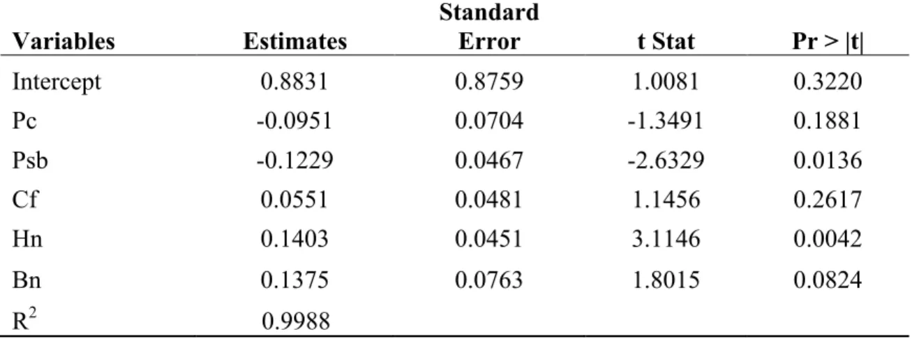
Table 16 shows that for every dollar increase in corn and soybean price, feed consumption will decrease by 0.0951 and 0.1229 million bushels respectively. Also, for every increase in the number of cattle, hogs and broilers on feed, there will be an increase in feed consumption by 0.0551, 0.1403, and 0.1375 million bushels respectively.
Table 16. Results of Feed Consumption (Million bushels) in the United States as a function of future corn price, soybean price, cattle on feed, number of Hogs, and number of broilers. Variables Estimates Standard Error t Stat Pr > |t| Intercept 0.8831 0.8759 1.0081 0.3220 Pc -0.0951 0.0704 -1.3491 0.1881 Psb -0.1229 0.0467 -2.6329 0.0136 Cf 0.0551 0.0481 1.1456 0.2617 Hn 0.1403 0.0451 3.1146 0.0042 Bn 0.1375 0.0763 1.8015 0.0824 R2 0.9988
Food, Alcohol and other Industrial Uses
In Table 17, we expect the coefficient of corn price to be negative and the ethanol production coefficient is expected to be positive as an increase in ethanol production is expected to increase ethanol use. The result shows that for every dollar increase in corn price, Food, Alcohol and other Industrial Uses (FAI) will decrease by 0.0846 million bushels.
Table 17. Results of Food, Alcohol and other Industrial Uses in the United States as a function of future corn price, Ethanol Production, Population and Trend.
Variables Estimates Standard Error t Stat Pr > |t| Intercept 103.7080 19.3718 5.3536 0.0000 Corn Price -0.0846 0.4280 -0.1977 0.8447 Eth Production 0.0232 0.0005 48.1167 0.0000 Pop -0.4187 0.0915 -4.5786 0.0000 Trend 2.1125 0.2442 8.6521 0.0000 Price Equation
The effect of each of these demand factors on corn price varies in terms of magnitude of their coefficients. The impact of FAI consumption on corn price is the greatest. Feed consumption is the next and last is export consumption. Both FAI and export consumption are significant at 5% level, while the impact of feed consumption on corn price is not statistically significant.
Increasing demand from FAI best explains corn price than other uses as shown in Table 18.
Table 18. Results of Corn price in the United States as a function of corn supply, Feed use, Food, Alcohol and other Industrial, Corn Export and Lagged Corn price.
Variables Estimates
Standard
Error t Stat Pr > |t|
Intercept 7.0758 1.3125 5.3911 0.0000
Corn Supply -0.0004 9.2E-05 -4.2726 0.0002
Feed use 0.0003 0.0003 1.2037 0.2392
FAI 0.0044 0.0010 4.4464 0.0001
Exports 0.0008 0.0002 3.2703 0.0029
Pct-1 0.2288 0.0916 2.4966 0.0189
R 0.9566
In Table 19, we expect real corn price to have a positive impact on harvested area, and soybean and wheat prices are expected to have a negative impact on harvested area since soybeans and wheat are competing crops. Table 19 shows that the U.S. corn price has a significant impact on acreage change in the United States. That is, for every $1.00 increase in corn and wheat price, there will be 0.2102 and 0.0724 (1,000HA) change in corn acreage in the United States.
Table 19. Results of Harvested Area (1,000HA) in the United States as a function of lagged harvested area, lagged corn price, soybean price and wheat price.
Variables Estimates Standard Error t Values Pr > |t| Intercept 1.5529 0.3535 4.3932 0.0001 Hat-1 0.2897 0.1391 2.0832 0.0448 Pct-1 0.2102 0.0835 2.5159 0.0168 Psbt -0.0491 0.0431 -1.1386 0.2628 Pwt 0.0724 0.0670 1.0811 0.2873 R2 0.4286
Table 20 shows that for every $1.00 increase in corn price, there will be no change in corn acreage in Brazil. And for every $1.00 increase in price of soybean and wheat, corn acreage will increase by 0.0163 and 0.0104 (1,000HA) respectively.
Table 20. Results of Corn Harvested Area in Brazil as a function of lagged harvested area, lagged corn price, soybean price and wheat price.
Variables Estimates
Standard
Error t -Values P-value
Intercept 0.4986 0.1514 3.2935 0.0023
Hat-1 0.5264 0.1398 3.7647 0.0006
Pwt 0.0104 0.0299 0.3464 0.7312
R2 0.4884
Table 21 shows that for every $1.00 increase in corn price, there will be no change in corn acreage in Canada. And for every $1.00 increase in price of soybean and wheat, corn acreage will increase by 0.0019 and 0.0003(1,000HA) respectively.
Table 21. Results of Harvested Area in Canada as a function of lagged harvested area, lagged corn price, soybean price and wheat price.
Variables Estimates Standard Error t Values Pr > |t|
Intercept 0.0240 0.0123 1.9576 0.0585 Hat-1 0.6995 0.1081 6.4737 0.0000 Pct-1 -0.0013 0.0011 -1.2320 0.2264 Psbt 0.0019 0.0019 0.9809 0.3336 Pwt 0.0003 0.0029 0.1154 0.9088 R2 0.8382
Table 22 shows that for every $1.00 increase in corn price, there will 0.0226 (1,000HA) change in corn acreage in the EU. And for every $1.00 increase in price of soybean and wheat, there will be no change in corn acreage.
Table 22. Results of Harvested Area in EU as a function of lagged harvested area, lagged corn price, soybean price and wheat price.
Variables Estimates Standard Error t Values Pr > |t|
Intercept -0.0161 0.05611 -0.2861 0.77653 Hat-1 0.96227 0.07781 12.3666 0.0000 Pct-1 0.0226 0.06007 0.37622 0.70909 Psbt -0.0058 0.01567 -0.373 0.71149 Pwt -0.0002 0.03449 -0.0072 0.99427 R2 0.8501
Table 23 shows that for every $1.00 increase in corn price, there will 0.0355 (1,000HA) change in corn acreage in Mexico And for every $1.00 increase in price of soybean , corn acreage will increase by 0.0005 (1,000HA).
Table 23. Results of Harvested Area in Mexico as a function of lagged harvested area, lagged corn price, soybean price and wheat price.
Variables Estimates Standard Error t Values Pr > |t| Intercept 0.2029 0.1042 1.9487 0.0596 Hat-1 0.7025 0.1282 5.4801 0.0000 Pct-1 0.0355 0.0446 0.7953 0.4319 Psbt 0.0005 0.0124 0.0406 0.9678 Pwt -0.0219 0.0249 -0.8778 0.3862 R2 0.4782
Table 24 shows that for every $1.00 increase in corn and soybean price, there will no change in corn acreage in Japan and for every $1.00 increase in price of wheat, corn acreage will increase by 0.0001 (1,000HA).
Table 24. Results of Harvested Area in Japan as a function of lagged harvested area, lagged corn price, soybean price and wheat price.
Variables Estimates Standard Error t Values Pr > |t|
Intercept 0.0006 0.0004 1.5749 0.1245 Hat-1 0.7963 0.0279 28.4519 0.0000 Pct-1 -0.0002 0.0004 -0.4654 0.6446 Psbt -8E-05 0.0001 -0.6575 0.5153 Pwt 0.0001 0.0002 0.65543 0.5166 R2 0.4782
Table 25 shows that for every $1.00 increase in corn and soybean price, there will no change in corn acreage in China and for every $1.00 increase in price of wheat, corn acreage will increase by 0.0333 (1,000HA). It is clearly shown in Table 20-25 shows that U.S. corn price does not have any significant impact on acreage change in countries like Brazil, Canada, Japan, and China.
Table 25. Results of Harvested Area in China as a function of lagged harvested area, lagged corn price, soybean price and wheat price.
Variables Estimates Standard Error t Values Pr > |t| Intercept 0.0426 0.1203 0.3546 0.7251 Hat-1 0.9819 0.0605 16.2356 0.0000 Pct-1 -0.0202 0.0849 -0.2374 0.8138 Psbt -0.0054 0.0220 -0.2465 0.8068 Pw t 0.0333 0.0483 0.6882 0.4959 R2 0.9331
These results indicate that with or without biofuel production, excess capacity still exists in corn production. Of the countries examined, Japan is the only country where acreage is seen to be most important in predicting corn production (Table 4). In the three demand equations (ethanol production, feed use and FAI), the corn price coefficient is negative as expected. Corn price was seen to have a negative impact on these uses of corn, as an increase in the price of corn decreases ethanol production, feed use and Food, Alcohol and Industrial uses (FAI).
The effect of each of these demand factors on corn price varies in terms of magnitude of their coefficients. The impact of FAI consumption on corn price is the greatest. Export is the next and last is feed consumption. Both FAI and export
consumption are significant at the 5% level, while the impact of feed consumption on corn price is not statistically significant. Based on this, we can say that increasing demand from FAI best explains corn price than other uses. The result shows that
increasing ethanol production in the US has a positive and significant relation to the U.S. corn price. Also, the U.S. corn price is positively and significantly related to change in land use system in the United States. But U.S. corn price has not impacted acreage change in the countries of Brazil, Canada, Japan, and China (Table 21 through 25).
Conclusion
This research primarily focused on the impact of United States corn based ethanol production on land use in Brazil. A series of equations were estimated using regression analysis. The result shows that increasing ethanol production in the U.S. has a positive and significant relation to the U.S. corn price. The U.S. corn price is not significantly related to changes in the land use system in Brazil. In contrast to what is written in most research work that ethanol production in the U.S. will increase corn prices which will result in land use changes in other countries, results do not suggest that ethanol
production in the US will result in total land use change, rather it suggests that ethanol production will impact price by increasing the price of corn and corn price will bring about a minimal change in land use. An increase in the corn price will have more of an impact on yield than acreage change, meaning there will be an increase in input used per acre as corn price increases rather than change in acreage. In countries like Brazil, Japan, China and Canada, a change in the price of corn does have an impact on acreage change. These countries do not depend on the U.S. corn market price to determine their
production.
To get the full understanding of the overall impact of ethanol production in the US on corn prices, future research work can look into the following areas:
• The difference in transportation cost between countries (transporting grain crops from one location to the other).
• The substitute between competing crops
• Different season of the year, to be able to know the planting season of corn maybe planting season varies across countries.
• The socio-economic study of where land is coming from in Brazil to better understand the type of land converted to cropland in Brazil (cropland or pastureland)
References
Ahmed, S.A., T.W. Hertel, and R. Lubowski. 2008. “Calibration of a Land Cover Supply Function Using Transition Probabilities.” GTAP Research Memorandum No. 14, Center for Global Trade Analysis, Purdue University. www.gtap.org.
Birur, D., T. Hertel, and W. Tyner. 2008. "The Biofuels Boom: Implications for World Food Markets." Dutch Ministry of Agriculture, January 9, 2008.
Bridges, D., and F. Tenkorang. 2009. Agricultural Commodities Acreage Value Elasticity over Time—Implications for the 2008 Farm Bill. Paper presented at the American Society of Business and Behavioral Sciences Annual Conference, Las Vegas, NV. Chambers, R. and R. Just. 1981. “Effects of Exchange Rate Changes on U.S.
Agriculture : A Dynamic Analysis” American Journal of Agricultural Economics 63(1).
Chavas, J.P., and M.T. Holt. 1990. “Acreage Decisions under Risk: The Case of Corn andSoybeans”. American Journal of Agricultural Economics. 72 (3): 529-538. Davison, C.W., and B. Crowder. 1991. “Northeast Soybean Acreage Response Using
Expected Net Returns.” Northeastern Journal of Agricultural and Resource Economics, 20 (1): 33-41.
De La Torre Ugarte, D. G., and D. E. Ray 2000. “Biomass and Bioenergy Applications of the POLYSYS Modeling Framework”, Biomass and Bioenergy 18(4), 291–308. De La Torre Ugarte, D.G., M.E. Walsch, H. Shapouri, and S.P. Slinsky. “The Economic
Impacts of Bioenergy Crop Production on U.S. Agriculture.” United States Department of Agriculture, February 2003:1-41.
Du, X., D.Hennessy, and W.A Edward (2008). “Does a Rising Biofuels Tide Raise All Boats? A Study of Cash Rent Determinants for Iowa Farmland under Hay and Pasture.’’Journal of Agricultural & Food Industrial Organization, 6:1-23. Elobeid, A., S. Tokgoz, and D.J. Hayes, B.A. Babcock, and C.E. Hart. 2006. “The
Long-Run Impact of Corn-Based Ethanol on the Grain, Oilseed, and Livestock Sectors; Preliminary Assessment.” CARD Briefing Paper 06-BP 4.
Fabiosa, Jacinto F., John C. Beghin, Fengxia Dong, Amani Elobeid, Simla Tokgoz, and Tun-Hsiang Yu. 2009. “Land Allocation Effects of the Global Ethanol Surge: Predictions from the International FAPRI Model.” Working Paper, Center for Agricultural and Rural Development,Iowa State University.
Fargione J., J. Hill, D. Tilman, S. Polasky and P. Hawthorne (2008): “Land Clearing and the Biofuel Carbon Debt”, Science 319 (5867): 1235-1238
Farrell, A.E., R.J. Plevin, B.T. Turner, and D.M. Kammen. 2006. “Ethanol Can Contribute to Energy and Environmental Goals.” Science 311: 506-508.
FAPRI (Food and Agricultural Policy Research Institute). 2004. Documentation of the FAPRI Modeling System. FAPRI-UMC Report # 12-04, University of
Missouri.http://www.fapri.missouri.edu/outreach/publications/2004/FAPRI_UMC _Report12_04.
Ferris, J., and S. Joshi. 2009. “Prospects for Ethanol and Biodiesel, 2008 to 2017 and Impacts on Agriculture and Food." ed. M. Khanna, J. Scheffran, and D. Zilberman, Springer.
Ferris, J. 2005. Agricultural prices and commodity market analysis. 2nd ed. East Lansing, MI: Michigan State University Press: 136–137.
Food and Agricultural Policy Research Institute at the University of Missouri-Columbus (FAPRI-MU). 2008. “FAPRI-MU model of the United States Ethanol Market.” FAPRI-MU Report # 07-08.
Fortenbery, T. Randall and Park, Hwanil. 2008. “The Effect of Ethanol Production on the U.S. National Corn Price.” Staff Paper No. 523, University of Wisconsin,
Department of Agricultural and Applied Economics.
Gardner, B.L. 1976. “Futures Prices in Supply Analysis”. American Journal of Agricultural Economics. 58 (1): 81-84.
Hayes, D., Babcock, B., Fabiosa, J., Tokgoz, S., Elobeid, A., Yu, T.-H., et al. (2009). Biofuels: Potential Production Capacity, Effects on Grain and Livestock Sectors, and Implications for Food Prices and Consumers. Journal of Agricultural and Applied Economics 41(2): 1-27.
Hertel, T.W., W.E. Tyner, and D.K. Birur. 2008. “Biofuels for all? Understanding the Global Impacts of Multinational Mandates” GTAP working paper 51, Center for Global Trade Analysis. Purdue
University.https://www.gtap.agecon.purdue.edu/resources/download/393.pdf Houck, J.P., and M.E. Ryan. 1972. “Supply Analysis for Corn in the United States: The
Impact of Changing Government Programs.” University of Minnesota Institute of Agriculture, P72-4.
Huang, W., M. R. Dicks, B. T. Hyberg, S. Webb and C. Ogg. 1988. “Land Use and Soil Erosion: A National Linear Programming Model.” U.S. Department of
Agriculture, Economic Research Service, Washington, DC. Technical Bulletin No. 1742.
Lee, D.R., and P.G. Helmberger. 1985. “Estimating Supply Response in the Presence of Farm Programs”. American Journal of Agricultural Economics. 67 (2): 193-203. Kanlaya J. Barr, Bruce A. Babcock, Miguel Carriquiry, Andre Nasser, and Leila Harfuch.
2010. “Agricultural Land Elasticities in the United States and Brazil.” CARD Working Paper 10-WP 505, Center for Agricultural and Rural Development, Iowa State University.
Keeney, R., and Hertel, T. 2008. “The Indirect Land Use Impacts of U.S Biofuel Policies: The Importance of Acreage, Yield, and Bilateral Trade Responses,” GTAP
Working Papers No. 52, Department of Agricultural Economics, Purdue University.
Murray, M. P. (2006). Econometrics: A modern introduction. Boston: Pearson Addison Wesley.
Mills, K., M.R. Dicks, D.Lewis, and R. Moulton. 1992. “Methods for Assessing Agricultural-Forestry Land Use Changes.” OAES Research Report P-928, Oklahoma State University.
Ray, D. E. and T. F. Moriak. 1976. “POLYSIM: A National Agricultural Policy Simulator.”Agricultural Economics Research 28(1), 14–21.
Reese, R. A., & Iowa State University. (1992). Biomass as sustainable energy: The potential and economic impacts on U.S. Agriculture. Ames, Iowa: Center for Agricultural and Rural Development, Iowa State University.
Reilly, J., A. Gurgel, and S. Paltsev. 2009. "Biofuels and Land Use Change." ed. M. Khanna St.Louis, MO, Farm Foundation.
Searchinger, T., Heimlich, R., Houghton, R. A., Dong, F., Elobeid, A., Fabiosa, J., et al. 2008. “Use of U.S. croplands for biofuels increases greenhouse gases through emissions from land-use change”. Science Express 319, 1238-1240.
Taylor, R., J. Mattson, J. Andino and W. Koo. 2006. "Ethanol's impact on the U.S. Corn Industry" North Dakota State University.
Tweeten, L.G., and C.L. Quance. 1969. “Positivistic Measures of Aggregate Supply Elasticities: Some New Approaches.” American Economic Review 59 (2): 175-183.
Wang, M. & Haq, Z. (14 March 2008) Letter to Science.
APPENDIX
Figure 1. US Corn Production (1,000MT) from 1960 to 2008.
Figure 2. US Corn Acreage (1,000HA) from 1960 to 2008.
US Corn Production (1,000 MT) 1960 1961 1962 1963 1964 1965 1966 1967
US Corn Acreage (1,000 HA)
1960 1961
Figure 3. Brazil Corn Production (1,000HA) from 1960 to 2008.
Figure 4. Brazil Corn Acreage (1,000HA) from 1960 to 2008.
Brazil Corn Production(1,000MT)
1960 1961