1
Optimal Coverage Level Choice with Individual and Area Plans of Insurance Harun Bulut, Keith Collins, and Tom Zacharias1
Selected Paper prepared for presentation at the Southern Agricultural Economics Association Annual Meeting, Corpus Christi, TX, February 5-8, 2011
Copyright 2011 by [Harun Bulut, Keith Collins, and Tom Zacharias]. All rights reserved. Readers may make verbatim copies of this document for non-commercial purposes by any means, provided this copyright notice appears on all such copies.
1 The authors are affiliated with the National Crop Insurance Services (NCIS), Overland Park, KS, and can be reached at harunb@ag-risk.org, kjcdog@msn.com , or TomZ@ag-risk.org , respectively.
2 Optimal Coverage Level Choice with Individual and Area Plans of Insurance
January 14, 2011
Harun Bulut, Keith Collins, and Tom Zacharias
Abstract: We theoretically examine a farmer’s coverage demand with area and individual insurance plans as either separate or integrated options. The individual and area losses are assumed to be imperfectly and positively correlated. With actuarially fair rates, the farmer will fully insure with the individual plan and demand no area insurance regardless of the plans being separate or integrated. Under separate plans, free area insurance and the fair rate for individual insurance, area insurance replaces a portion of individual insurance demand. Under integrated plans, free area insurance, and the fair rate for individual insurance, the farmer over-insures using both area and individual plans.
Key words: Agricultural risk, area plans of insurance, crop insurance
3 The Federal Crop Insurance (CI) program has grown to become the centerpiece of the
agricultural safety net for crops and currently protects nearly $80 billion worth of liability. Government spending on crop insurance is now projected to exceed spending on farm
commodity programs in future years (Shields, Monke and Schnepf, 2010). With all farm support programs expected to face tight budget constraints in the upcoming Farm Bill, alternative
programs are under examination to reduce spending, simplify programs, and eliminate
redundancy. Therefore, it is imperative to examine the interaction of crop insurance and other farm support programs and assess how producers may be affected by emerging Farm Bill proposals for alternative farm support structures.
A key development in the last Farm Bill was the move toward revenue protection as an objective of traditional farm programs. Early proposals for the next Farm Bill have included variations on the role of revenue protection in farm programs, with an emphasis on improved area revenue protection. However, most crop insurance policies sold today provide revenue protection on either a county or individual basis. This situation is raising fundamental questions about the effectiveness for producers of area versus individual revenue protection plans, with such plans used either separately or in combination with one another. Consequently, the focus of this article is on the connection between individual and area plans of crop insurance and current and proposed area revenue plans under farm programs. We address this issue by deriving the producer’s preference for coverage among the various area and individual plans of revenue protection by using an economic model of producer choice. We present conclusions from the model on a producer’s choice and discuss these in the context of the economic literature on area plans.
4 area revenue programs. Since the 1990s, farmers have had both individual farm and county-based Revenue Insurance Plans available within the CI program, which protect against revenue shortfalls. The CI revenue plans currently constitute nearly the 80% of total premium. The Food, Conservation, and Energy Act of 2008 (2008 Farm Bill) authorized additional farm programs to protect revenue. One plan, the Supplemental Revenue Assistance Payments Program (SURE), is a whole farm program that supplements CI and the Noninsured Crop Disaster Assistance
Program. Payments under SURE are based on individual producer losses over an entire farm. However, the other new plan, Average Crop Revenue Election (ACRE), protects against revenue shortfalls at the state level. Some concerns on possible overlap and duplication of coverages between ACRE and CI have been raised (Zulauf, Schnitkey and Langemier, 2010; Barnaby, 2010).
There are also proposals emerging for changing ACRE into a county-level area plan and integrating that with crop insurance (Babcock, 2010). Integrated programs are also known as “wrapped insurance,” where individual insurance works as if “wrapped” around the area
program only paying when an individual’s indemnities exceed payments from the area program. Individual crop insurance would pay the residual amount once area payments are netted out (Coble and Barnett, 2008). Similarly, Cooper (2010) includes ACRE payments in the harvest-time premium calculation for CI.
A solid understanding of the interaction of CI with area insurance and related revenue programs and how these options address the risk management needs of producers and affect their participation decisions is essential for a healthy public policy discussion. However, the literature developing the factors behind a producer’s choice of area insurance, such as Miranda (1991) and
5 Mahul (1999), has not taken into account the availability of multiple insurance or farm program alternatives in the analytical modeling.
In order to extend past research on producer choice to better incorporate policy choices that might be considered for the upcoming Farm Bill discussions, we developed a stylized analytical model to assess a farmer’s choice of coverage levels from individual and alternative area plans of insurance. We combined the two-point distribution approach used in the Duncan and Myers (2000) insurance model with the correlation modeling approach used in Bulut and Moschini (2006). The model is flexible to accommodate existing insurance plans such as the yield-based Group Risk Plan (GRP) or the revenue-based Group Risk Income Protection (GRIP) and current or proposed farm revenue protection programs (such as the current ACRE or a county-based ACRE).
We identify the main factors determining the farmer’s coverage demands as: the premium rates, expected farmer’s and area losses, standard deviations of farmer’s and area losses, the correlation between farmer’s and area losses, and the farmer’s degree of risk aversion. Overall, the findings indicate a strong case for individual insurance vis-à-vis area insurance when the premium rates for area and individual plans are actuarially fair (equal to expected indemnities).
The theoretical model provided here may help evaluate the effectiveness of proposed county-level area plans from a pure risk management perspective. The model can be useful to explain the pattern of actual coverage in counties where ACRE participation is low or high. It also helps explain regional participation levels in county-level insurance plans, such as the yield-based Group Risk Plan (GRP) or the revenue-yield-based Group Risk Income Protection (GRIP).
The paper is organized as follows. The next section introduces the model. The insurance decision of the farmer is analyzed in the following contexts as subsections: 1) solely with an
individual plan of insurance; 2) solely with an area plan of insurance; 3) with either an individual or an area plan of insurance but not both simultaneously; 4) with separate area and individual plans of insurance that may be held either alone or simultaneously; 5) with integrated area and individual plans of insurance that may be held either alone or simultaneously. At each
subsection, the results are provided. Following is a discussion of our findings in connection with the related literature. Finally, in the last section, we present the major conclusions.
Modeling
As in Duncan and Myers (2000), the farmer has a mean-variance utility function, pays a
premium and chooses coverage levels. In addition, we introduce area insurance plans and define the joint distribution of individual and area losses where the losses are imperfectly and positively correlated. The correlation modeling approach used in Bulut and Moschini (2006) is adopted here. We then solve a risk-averse farmer’s optimization problem under various insurance plan options.
Insurance Decision with Individual Plan of Insurance
Duncan and Myers (2000) formulated a farmer’s insurance demand without considering area-based insurance. Their framework is adopted here. The farmer faces the prospect of a loss (denoted with l) with probability pl and no loss with probability (1−pl). Then, the expected loss (l ) and the variance of loss (σl2) can be obtained as
l l = pl l (1) 2 2 (1 ) l l pl p σ = − (2) 6
The farmer is assumed to have a linear mean-variance preference function2 specified as 2 0.5 i i x i U =M−π x− −l λσl (3)
where Udenotes utility, M : the farmer’s initial income, πx: premium per unit of insurance coverage level, x: coverage level, li: the farmer’s expected loss with coverage, λ: risk aversion parameter, 2
i l
σ : variance of the farmer’s expected loss with coverage.
If a farmer holds x units of coverage with individual insurance, then the expected indemnity (denote with R(i ) would be
i l
R( =xp l =xl (4)
The expected loss of farmer with coverage would be i
(1 ) (1 )
i l l l
l( = −x l = −x p l= p l−xp l= −l Ri
(
(5)
And the variance of the loss of the farmer when the farmer has coverage units of x would be
2 2 2 2 2 (1 ) (1 ) (1 ) i l x l x l pl pl σ = − σ = − − (6) 2
The mean-variance model was also used in the literature studying area insurance such as Miranda (1991) and Barnett et al. (2005). These studies assume actuarially fair rates so that maximizing mean-variance utility reduces to minimizing the variance. Meyer (1987) shows that mean-variance utility maximization is equivalent to expected-utility maximization under a sufficient condition (the location and scale parameter condition), which tends to hold in many economic models. Whether the location and scale parameter condition holds for crop insurance losses (yield or revenue) in particular is an empirical question which can be investigated along the lines of Antle (2010).
The farmer’s problem is to maximize the utility function in equation (3) by choosing a non-negative level of coverage x.3 The necessary and sufficient first-order condition (F.O.C.) to solve this problem is
2 (1 ) l 0
l x
π λ σ
− + + − = (7)
Solving this condition yields demand for insurance as
2 1 x l l x π λσ − + = + ( (8)
The demand for coverage decreases with the increases in premium πx and increases with increases in the expected loss l . If the insurance is actuarially fair, that is, premium rate equals expected loss, πx =l so that the premium amount would equal expected indemnity in equation (4), then the strictly risk averse individual will insure completely (x(=1).4 If the premium rate is
x l
π > , that is, rates are unfair (overrated), the demand for coverage will be less than one and increasing with the risk aversion parameter λ and the variance of loss 2
l
σ . Note that premiums for insurance other than Federal crop insurance typically involve an expense load, which may cause the premium rates to be higher than the expected indemnity. If insurance is underrated, that
3 Similar to Duncan and Myers, a deductable or co-insurance is not considered because the probability of loss is assumed to be unaffected by the individual’s actions. One possible extension here would be to consider possibility that the individual can affect the probability of loss through some effort.
4 See also Example 6.C.1. on page 187 in Mas-Colell, Whinston, and Green (1995).
is, πx<l , then the demand for coverage will exceed one (over-insurance) and be decreasing with the risk aversion parameter λ and the variance of loss σl2.
Introducing the Area Plans of Insurance
Suppose that area insurance is available and pays whenever there is a loss at the area level. Denote the amount of area loss with L and probability of loss for the area with pL. One can verify that the expected area loss (denoted with L) and the variance of the area loss (denoted with σL2) are L L = p L (9) 2 2 (1 ) L L pL pL σ = − (10)
Denote the coverage demanded for area insurance with yand the associated premium per unit of coverage with πy. If the farmer holds units of coverage from area insurance, then the farmer’s expected loss solely from area loss
y
(
i L )
L = yp −L
(11)
which is the negative of the expected indemnity with area insurance. Moreover, the variance of farmer’s loss with area coverage would be
2 2 2 2 2
(1 )
i
L y L y L pL pL
σ = σ = − . (12)
In the next section, we define the joint distribution between individual and area losses.
The Joint Distribution of the Individual and Area Losses
The joint distribution of the individual and the area losses is as follows. Denote the random outcome of whether a loss occurred for the farmer and the area with Xi and Xa, respectively. Then, the events possible (X Xi, a) are: both individual and area see a production loss, ; individual sees a loss but area does not, (1, ; individual does not see a loss but area does, (0 ; and neither individual nor area sees a loss, . The probability matrix for these events is
(1,1) ,1)
0) (0, 0)
Area with a loss (1) Area without a loss ( ) 0
Individual with a loss (1) plL plN
Individual without a loss ( ) 0 pnL pnN
Then, the probabilities for joint events can be written as
lL l L l L
p = p p +ρr r (13)
(1plN = pl −pL)−ρr rl L (1pnL = −p pl) L−ρr rl L (1pnN = −pl)(1−pL)+ρr rl L
where ρ is the correlation coefficient, is the standard deviation of event rl Xi and is the standard deviation of event
L
r
a
X and the standard deviations are defined as
(1 ) l l r = p −pl (14) (1 ) L L r = p −pL (15)
In addition, the covariance term between the events (X Xi, a) is in equations (13) and equal to ( i, a) l
Cov X X =ρr rL (16)
Note that the value of the correlation coefficient parameter must be consistent with the fact that probabilities in equation (13) are all non-negative. We further assume that and . From these relationships, one can re-obtain the marginal probability of losses as
0 lN p > pnL >0 l lL lN p = p +p (17) L lL nL p = p +p
Insurance Decision for either Individual or Area Plans of Insurance
This decision is similar to the choice between the county insurance plan GRP versus an individual APH yield insurance plan. The producer cannot have both the area plan and the individual plan at the same time. Having derived the demand for coverage with an individual plan in equation (8), we obtain the coverage demand for an area insurance plan next.
The expected loss when the farmer holds units of coverage solely from area insurance would be
y
i l L L
l( = p l−p yL= −l p yL (18)
And the variance of the farmer’s loss when the farmer solely holds coverage with area insurance would be 12 2 2 2 2 2 i l plL l yL li plN l li pnL yL li pnN li σ( = ⎣⎡ − −(⎤⎦ + ⎡⎣ −(⎤⎦ + ⎡⎣− −(⎦⎤ + ⎣⎡−(⎤⎦ (19) Plugging the expression for l(from equation (18) in equation (19), one can obtain
2 2
i
l l
σ( =σ +ε(. (20)
where ε( is the risk reduction that can be obtained by holding coverage with area insurance and equal to 2 2 2 L l y y L ε(= σ − ρσ σ (21)
The farmer’s decision problem is 2 0 0.5 i i y i y Max U M π y l λσl ≥ = − − −( ( ( . (22)
The necessary and sufficient F.O.C for the preceding problem is 2 0.5 li i i y U l y y y σ π λ∂ ∂ ∂ = − − − ∂ ∂ ( ( ∂ . (23)
From equations (18) and (20), one obtains
i L l p L y ∂ = − ∂ ( (24)
2 2 2 2 i L L l L y y σ σ ρσ σ ∂ = − ∂ ( . (25)
Plugging the corresponding expressions in (23) and solving yields
2 y l L L L y π ρσ λσ σ − + = + ( . (26)
When the area insurance rates are actuarially fair, that is, πy=L, then the demand for area
insurance becomes y l L L yπ ρσ σ = = ( . (27)
The risk-reduction can be obtained with y( (after plugging y( from equation (27) in equation (21)) is
2 2
l
ε(= −ρ σ . (28)
The expression in equation (27) was also derived in Miranda (1991) (see equation (13) on page 235) and is known as the farmer’s β. The farmer seeks higher coverage with an area plan the higher the correlation between the individual and area losses, the higher the farmer’s own risk (σl ), and the lower the variance of area loss. In particular, if σl >σL and the correlation is also sufficiently high so that ρσl >σL, then it would be optimal to set 1
y L
y
π = >
( .
Proposition 1. If the farmer can hold coverage from either individual or area insurance, the farmer will prefer to hold coverage with individual insurance rather than area insurance when
the premium rates are actuarially fair, that is, (πx=l for individual insurance and πy =L for area insurance). The utility level under individual coverage will be ( )
x
i l
U x( π = =M −l .
Given the premium rates are actuarially fair, the farmer wants to minimize the variance of loss. With individual insurance, the farmer can minimize that risk to zero by fully insuring which can be verified from equation (6). However, with area insurance, the farmer cannot do the same unless the farmer’s and area losses are perfectly correlated, which can be verified from equation (28).
Deng, Barnett, and Vedenov (2007) claim that premium rates for MPCI yield plans have large positive “wedges”, that is, they are over-charged and are not actuarially fair due to moral hazard and adverse selection problems (see page 518 in their paper). If the rate for individual insurance is over-charged, then the demand for coverage with individual insurance in equation (8) is less than 1, that is, less than full insurance. Assuming the fair rate for area insurance, for a sufficiently high level of over-charge in individual insurance, one can verify that the area insurance could indeed be preferred over individual insurance.
Insurance Decision for Area and Individual Plans of Insurance
In this framework, the farmer pays premium for both individual and area plans, and can have both the area and individual plans simultaneously. This situation is similar to the state ACRE program, where the producer pays an implicit premium (gives up a portion of Direct Payments and marketing loans). Our framework is more general because the farmer can choose
coverage levels from both plans. In addition, unlike the ‘double trigger” requirement in ACRE, our framework allows for the possibility that the farmer can be paid when the area has a loss but not the farmer, which is in line with GRP or GRIP plans of insurance. The latter makes the area insurance more desirable from farmer’s point of view.
With the possibility of holding coverage from area and individual level insurances, the farmer’s objective function becomes
15 l 2 0 0 ˆ ˆ 0.5 ˆ i i x y i x y MaxU M π x π y l ≥ ≥ = − − − − λσ (29) where and lˆi 2 ˆ i l
σ will be defined in the following. Using the relations in equations (5), (11), (13) and (17), one can obtain the expected indemnity for farmer i who is covered with both
individual and area insurance. The expected indemnity (denote with ) under separate plans can be defined as ˆ i R
[
]
[ ]
[ ]
[ ]
ˆ 0 i lL lN nL nN l L R p xl yL p xl p yL p p xl p yL = + + + + = + (30)Then, one can verify that the expected loss (denote with ) would be lˆi
[
]
[
]
[
]
[ ]
ˆ (1 ) ( ) (1 ) ( ) 0 ˆ (1 ) ( ) i lL lN nL nN l L i l p x l y L p x l p y L p p x l p y L l R = − + − + − + − + = − + − = − (31)Note that comparing equations (5) and (31), the additional coverage from area insurance decreases the farmer’s expected loss because of the higher expected indemnity, that is, comparing equation (4) and (30) yields ˆRi >R(i whenever y>0.
The variance of the farmer’s loss when holding coverage from both individual and area insurance is 16 ˆ 2 2 2 2 ˆ ˆ ˆ 2 ˆ (1 ) (1 ) (0 ) i l plL x l yL li plN x l li pnL yL li pnN li σ = ⎡ − − − ⎤ + ⎡ − − ⎤ + ⎡− − ⎤ + ⎡ − ⎣ ⎦ ⎣ ⎦ ⎣ ⎦ ⎣ ⎤⎦ (32)
where is as defined in equation lˆi (31). The preceding equation can be re-expressed in terms of the unconditional variance of the farmer’s loss from the individual plan (σl2) in equation (2) and the variance of the farmer’s loss from area insurance (σL2) in equation (10) and the covariance of discrete random outcomes for the individual and area (Cov(X Xi, a)) as
2 2 2 2 2 ˆ (1 ) 2(1 ) ( , ) i l x l y L x lyLCov Xi a σ = − σ + σ − − X l L (33) Inserting the covariance term from equation (16) in the preceding equation yields:
2 2 2 2 2
ˆ (1 ) 2(1 )
i
l x l y L x lyL r r
σ = − σ + σ − − ρ (34)
where and rl rL are defined in equations (14) and (15). The preceding equation can be re-expressed as 2 2 2 2 2 ˆ (1 ) 2 (1 ) i l x l y L x ly L σ = − σ + σ − ρ − σ σ 2 2 (35)
The preceding equation can be re-arranged as ˆ
ˆ
i
l l
σ =σ +ε (36)
where ˆε is the amount of risk-reduction that can be obtained by holding coverage with individual and/or area insurance plans:
17 2 2 2 2 2
ˆ x l 2x l y L 2 (1 x) ly L
ε = σ − σ + σ − ρ − σ σ (37)
The farmer will maximize utility by choosing coverage level x from individual insurance and coverage level y from area insurance. Differentiating the objective function in equation (29) with respect to the decision variables x and y, the necessary and sufficient5 first-order
conditions can be obtained as 2 ˆ ˆ 0.5 li 0 i x U l x x x σ π λ∂ ∂ = − −∂ − = ∂ ∂ ∂ (38) 2 ˆ ˆ 0.5 li 0 i i y U l y y y σ π λ∂ ∂ ∂ = − − − = ∂ ∂ ∂
From equation (31), one obtains ˆ i l l x ∂ = − ∂ (39) ˆ i l L y ∂ = − ∂
Also from equation (35), 2 l L 2 ˆ 2(1 ) 2 i l l x y x σ σ ρσ σ ∂ = − − + ∂ (40)
18 2 2 ˆ 2 2 (1 ) i l L l L y x y σ σ ρ σ ∂ = − − ∂ σ
Plugging the terms in equations (39) and (40) back into the F.O.C.s in equation (38) and solving for the demand for coverage in individual insurance and area insurance yields the following:
2 2 ( ) ( ) ˆ 1 (1 ) (1 ) y x l l L L l x π ρ π 2 λσ ρ λσ σ ρ − − = + − − − (41) 2 2 ( ) ( ) ˆ (1 ) (1 ) y x L l L L l y π ρ π 2 λσ ρ λσ σ ρ − − = − − −
Lemma 1. The coverage demands for individual and area insurances are substitutes whenever the area and individual losses are positively and imperfectly correlated, that is, 0< <ρ 1.
One can verify from equation (41) that the demand functions have positive cross-price derivatives whenever the correlation level is positive.
Proposition 2. Assume that area and individual losses are positively and imperfectly correlated, that is, 0< <ρ 1. If the rates for individual and area insurance are fair, that is, πx=l and
y L
π = , then the individual will fully insure with individual insurance (xˆ=1) and demand no area insurance, ( yˆ=0 ).
The proof is straightforward after plugging the actuarially fair premiums into equation (41). Because the premium rates are fair, the farmer’s problem reduces to minimizing the risk. The farmer can achieve full reduction in risk by fully insuring with individual insurance and none with area insurance, which can be verified from equation (37).
The following proposition provides the solution when area insurance becomes free, and individual insurance has the fair rate.
Proposition 3. If the premium for individual insurance is fair, that is, πx=l and the area insurance comes as free, that is, πy =0, then the individual will under-insure with individual insurance (that is, xˆ<1, therefore, xlˆ <l) whenever the individual and area losses are positively and imperfectly correlated, that is 0< <ρ 1. Specifically, the demand functions are:
2 ˆ 1 (1 ) l L L x ρ λσ σ ρ = − − (42) 2 2 ˆ (1 ) L L y λσ ρ = −
The following provide some comparative-statics results with respect to the parameters of the farmer’s problem such as the correlation level, amount of farmer’s loss, the degree of risk aversion, and amount of area loss.
Corollary 2: Assume that the premium for individual insurance is fair, that is, πx =l , the area insurance is free, that is, πy =0, and the area and individual losses are positively and
imperfectly correlated, that is, 0< <ρ 1. The demand functions at these rates are given in equation (42).
(1) The demand for individual insurance is decreasing when the correlation between area
loss and individual loss is increasing. That is,
0 ˆ 0 x y l x π π ρ = = ∂ <
∂ . The demand for area
insurance is increasing as the ρ becomes more positive, that is,
0 ˆ 0 x y l y π π ρ = = ∂ > ∂ .
(2) The demand for individual insurance is increasing when the amount of individual loss is
increasing, that is, 0 ˆ 0 x y l x l π π == ∂ >
∂ . The demand for area insurance is independent of the amount of individual loss.
(3) The demand for individual insurance coverage is increasing whereas the demand for
area insurance coverage is decreasing as the individual becomes more risk averse, that
is, 0 ˆ 0 x y l x π π λ = = ∂ > ∂ and 0 ˆ 0 x y l y π π λ = = ∂ <
∂ . Moreover, in the limit 0 ˆ lim x 1 y l xπ λ→∞ π == = and 0 ˆ lim x 0 y l yπ λ→∞ π == = .
(4) The demand for individual insurance is independent of the amount of area loss. Whereas
the demand for area insurance is decreasing as the amount of area loss is increasing,
that is, 0 ˆ 0 x y l y Lπ π == ∂ < ∂ .
The intuition for the first result is that when area insurance is free (or its rate becomes lower than the fair rate), the risk-averse farmer can tolerate a certain level of positive variance on income by balancing it with some gain in expected income, and can start demanding positive coverage with area insurance. The second and third results are pretty straightforward. The last
result can be counter-intuitive. When the amount of area loss increases, two things happen. First, because the area insurance is free, increasing amount of area loss increases expected indemnity from area insurance, therefore, the farmer’s expected income increases. However, increasing amount of area loss also increases the variance of farmer’s loss from equation (12). Because the second effect outweighs the first one, the farmer decreases its coverage with area insurance.
With the availability of free area insurance while individual insurance has the fair rate, the farmer may want to over insure, that is, the farmer may want to hold more coverage in total than what is necessary to pay the entire loss. The following characterizes the over-insurance. Recall that for a farmer with coverage levels x from the individual plan and from the area plan, then the indemnities under individual and area plans become
y
xl andyL, respectively. Corollary 3: Assume that the premium for individual insurance is fair, that is, πx =l , the area insurance comes as free, that is, πy =0, and the area and individual losses are positively and imperfectly correlated, that is, 0< <ρ 1. The demand functions at these rates are given in equation (42).
(1) If rl =ρrL, then xlˆ +yLˆ =l , that is, for all λ the farmer will fully insure using both individual and area insurance. If rl >ρrL, then xlˆ +yLˆ >l , that is, for all λ, the farmer will over-insure using both individual and area insurance. If rl <ρrL, then
ˆ ˆ
xl+yL<l , that is, for all λ the farmer will under-insure using both individual and area insurance.
(2) Moreover, consider the following threshold levels of λ:
1 2 ˆ (1 ) L L l p l r r ρ λ ρ = − (43) 2 2 1 ˆ (1 ) L L L p l r r λ ρ = − 1 2 ˆ ˆ ˆ λ λ λ= + Note that 1 2 ˆ ˆ L l r r λ ρ
λ = , which implies λˆ1 is greater, equal, or less than λˆ2 depending on
whetherρrL is greater, equal, or less than , respectively. Note also that: if rl λ λ= 1, then xˆ=0, and xˆ>0 implies λ λ> 1 . Then, depending on the magnitude of the degree of risk aversion relative to other parameters, the following hold:
i. If
λ λ
> ˆ , then 0<yLˆ <xlˆ <l. ii. Ifλ λ
= ˆ, then 0<xlˆ =yLˆ <l.iii. If max{ ,λ λˆ ˆ1 2}< <λ λˆ, then 0<xlˆ <yLˆ <l.
iv. Ifλ1>λ2⇔ρrL >rl and λ λ> ˆ1, then 0<xlˆ <yLˆ <l.
22 v. If λ1 <λ2⇔ρrL <rl and λ λ= ˆ2 , then 0<xlˆ <yLˆ =l.
vi. If λ1 <λ2⇔ρrL <rl and λˆ1< <λ λˆ2 , then 0<xlˆ < <l yLˆ .
Finally, the overlap between area insurance and individual crop insurance payments would be
the excess amount of indemnities over the farmer’s loss, that is, max{(xlˆ +yLˆ )−l, 0}.
Note that the claims (2.i) and (2.vi) above together with the limit result in claim (3) in Corollary 2 indicate that as the farmer gets more risk-averse, the farmer will choose higher coverage and therefore expected indemnities with the individual plan relative to the area plan.
Insurance Decision for the Integrated Individual and Area Plans of Insurance
In integrated programs, area payments offset crop insurance indemnities (Babcock, 2010). Integrated programs are also known as “wrapped insurance” where individual insurance works as if it is “wrapped” around area insurance because it only pays when individual
indemnities exceed area level indemnities and pays the residual amount once area payments are netted out (Coble and Barnett, 2008). In line with this, we define the individual insurance indemnities netted out from area payments as
23 0}
{ ,
Max xl yL
Δ ≡ − (44)
Note that xl≥ Δ ≥0. Also, whenever Δ =0, area payments totally offset the individual insurance payments. One can obtain the expected loss of the farmer under the integrated program as (denote with ) as l%i
[
]
[
(1 )]
[
( )]
[ ]
0i lL lN nL nN
l% = p l− Δ −yL + p −x l +p y −L +p (45)
Note that compared to the farmer’s expected loss with coverage with separate plans given in equation (31),
[
]
ˆ
i i lL
l% = +l p xl− Δ (46)
Therefore, expected loss at the same coverage levels is higher under the integrated plans compared to the one under separate plans. This is because the expected indemnity under integrated plans is lower than that under separate plans, which can be verified as follows:
The expected indemnity with integrated plans (denote with R%i ) as
[
]
[ ]
[ ]
[ ]
0i lL lN nL nN
Then, the expected loss of the farmer i from equation (45) can be re-expressed as
i l i
l% = p l−R% = −l R%i (48)
Using equations (30), (46) and (47), one obtains that
[
]
ˆi lL i
R% = p Δ −xl +R (49)
From equation (44), it follows that R%i <Rˆi.
Furthermore, the variance of the farmer’s loss when the farmer holds coverage from both individual and area insurance under the integrated program is
2 2 2 2 2 (1 ) (0 ) i l plL l yL li plN x l li pnL yL li pnN li σ% = ⎣⎡ − Δ − −%⎤⎦ + ⎣⎡ − −%⎦⎤ + ⎡⎣− −%⎦⎤ + ⎣⎡ −% ⎤⎦ (50)
where is as defined in l%i (46). Plug equations (32) and (46) into equation (50) and obtain 2 2
i
l l
σ% =σ +ε%
(51)
where ε% is the risk-reduction that can be obtained under integrated plans and can be written as,
[
]
[
]
[
]
2ˆ 2plL(1 p ll) (1 x xl) 2plL(1 pL)yL xl plL(1 plL) xl
ε ε%= + − − − Δ − − − Δ + − − Δ (52)
where ˆε is the risk-reduction can be obtained under separate plans from equation (37). Note that ε% can be lower or greater than ˆε (therefore, σ%l2i in equation (51) can be higher or lower than
2 ˆ
i l
σ from equation (36)) depending on the coverage levels x and y, and other parameters.
Then, the farmer’s problem can be written as
25 l 2 0 0 0.5 i i x y i x y MaxU M π x π y l ≥ ≥ = − − − −% % λσ% (53)
where U%i is the utility function of the farmer under integrated programs, and and l%i 2
i l
σ% are defined in equations (46) and (51), respectively. Note that the formulations of and l%i 2
i l
σ% , and therefore, the objective function depend on whether Δ =0 or Δ >0. Our solution strategy is to divide the problem in equation (53) into two sub-problems by assuming Δ =0(Assumption 1 below) and (Assumption 2 below) and finally combining the solutions obtained based on these assumptions in order to find the optimum for the original problem in equation
0 Δ >
(53). Assumption 1: Assume indemnities under the individual plan are lower than that under area plan, that is, xl−yL≤0, which implies that Δ =0. Plugging Δ =0 in equations (46) and (51) would yield expressions for the farmer’s expected loss with coverage (denote with ) and variance of the farmer’s losses with coverage (denote with
,1 i l% 2 ,1 i l σ% ) , respectively as follows: ,1 ˆ i i lL l% = +l p xl 2 2 (54) ,1 1 i l l σ% =σ +ε% (55)
[ ]
[ ]
[ ]
2 1 ˆ 2plL(1 p ll) (1 x xl) 2plL(1 pL)yL xl plL(1 plL) xl ε% = +ε − − − − + − (56)where ε%1 is the level of risk-reduction can be obtained under Assumption 1, and and lˆi εˆ are defined in equations (31) and (37), respectively. Plugging l%i,1 and 2,1
i l
σ% back in equation in (53) would yield an expression for the objective function:
26 l 2 ,1 1 1 ,1 0.5 i,1 i x y i U =M −π x −π y −l% − λσ% (57)
Assumption 2: Assume indemnities under the individual plan are higher than under the area plan, that is, xl−yL≥0, which implies that Δ = −xl yL≥0. Similarly, plugging
xl yL Δ = − 2 ,2 i l
into equations (46) and (51) would yield expressions for the farmer’s expected loss (denote with l%i,2) with coverage and variance of the farmer’s losses with coverage (denote with σ% ) as follows: ,2 ˆ i i lL l% = +l p yL (58) 2 2 ,2 2 i l l σ% =σ +ε% (59)
[ ]
[ ]
[ ]
2 2 ˆ 2plL(1 p ll) (1 x) yL 2plL(1 pL)yL yL plL(1 plL) yL ε% = +ε − − − − + − (60)where ε%2 is the level of risk-reduction can be obtained under Assumption 2, and and lˆi εˆ as defined earlier.
Plugging l%i,2 and 2,2
i l
σ% back into equation in (53) would yield an expression for the objective function: 2 ,2 2 2 ,2 0.5 i,2 i x y i U =M −π x −π y −l% − λσ%l (61) To summarize, Assumption 1 yields the objective function given in equation (57) and Assumption 2 yields the one in equation (61). Each objective function is assumed to be concave over the entire domain of ( , )x y , which is the non-negative orthant of real numbers. Then, the Hessian Matrix for each objective function is assumed to be negative definite (see also the
denominator terms in Tables 1 and 2). Each objective function is initially maximized over the entire domain of ( , )x y as if it is an unconstrained problem. A solution obtained by solving the necessary and sufficient F.O.C.s will maximize the given objective function over the entire domain. The resulting solutions are referred as ‘interior solutions’ below. Nevertheless, there is no guarantee that the interior solutions would satisfy the assumption from which the associated objective function is derived. Against this possibility, the objective functions in equations (57) and (61) are also maximized under the constraint of xl=yL. The resulting solutions are referred as ‘boundary solutions’ below. As a result of this process, the following solution candidates for the maximization of the original problem in equation (53) are obtained.
From Assumption 1 with the objective function in equation (57): The interior solution (denote with x y% %1i, 1i):
27 1 ( plL ) 1 i x y x% =⎣⎡ l − l −π δ⎦⎤ +⎣⎡L−π δ⎦⎤ 2+δ0 (62) 1 1 ( ) 2 i y lL x y% = L−π β +⎡⎣ l −p l −π β⎤⎦ + 0 b β ⎡ ⎤ ⎣ ⎦
The boundary solution (denote with x% %1b,y1) :
1 ( plL ) 1 b x y x% =⎡⎣ l − l −π η⎤⎦ +⎡⎣L−π η η⎤⎦ 2+ 0 (63) 1 2 ( ) 1 0 b y lL x l l l y L l p l L L L π η ⎡ π ⎤ η = − +⎣ − − ⎦ % ⎡⎣ ⎤⎦ η +
Table 1 depicts the coefficients (δ0 , β0 and η0 as the intercept terms; δ1, β1 and η1 as the own-price effects; and δ2, β2, and η2 as the cross-price effects ) in these solutions.
From Assumption 2 with the objective function in equation (61): The interior solution (denote with 2i
x% , 2i ): y% 2 1 i x y lL x% =⎡⎣l −π θ⎦⎤ +⎡⎣L−π − p L⎦⎤θ2+θ0 (64) 2 1 i y lL x y% =⎡⎣L−π −p L⎦⎤κ +⎡⎣l −π κ⎤⎦ 2+κ0 b
The boundary solution (denote with x% %2b,y2):
2 1 ( ) b x lL y x% =⎡⎣l −π ϕ⎤⎦ +⎣⎡ L−p L −π ⎦⎤ϕ ϕ2+ 0 (65) 2 ( ) 2 b lL y x l l y L p L l 1 l 0 L L L π ϕ ⎡ π ⎤ ϕ ⎡ ⎤ =⎣ − − ⎦ +⎣ − ⎦ + % ϕ
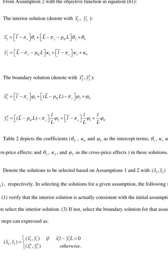
Table 2 depicts the coefficients (θ0 , κ0 and ϕ0 as the intercept terms; θ1, κ1 and ϕ1 as the own-price effects; and θ2, κ2, and ϕ2 as the cross-price effects ) in these solutions.
Denote the solutions to be selected based on Assumptions 1 and 2 with ( ,x y% %1 1) and 2 2
(x y% %, ), respectively. In selecting the solutions for a given assumption, the following steps are taken: (1) verify that the interior solution is actually consistent with the initial assumption. (2) If so, then select the interior solution. (3) If not, select the boundary solution for that assumption. These steps can expressed as:
1 1 1 1 1 1 1 1 ( , ) 0 ( , ) ( , ) . i i i i b b x y if x l y L x y x y otherw ⎧ − < = ⎨ ⎩ % % % % % % % % ise (66) 28
2 2 2 2 2 2 2 2 ( , ) 0 ( , ) ( , ) . i i i i b b x y if x l y L x y x y otherw ⎧ ise − > = ⎨ ⎩ % % % % % % % %
Then (4) the objective function given in equation (57) is evaluated at ( ,x y% %1 1)(denote the resulting value with U%i,1=Ui,1( ,x y% %1 1)) and the objective function given in equation
)
(61) is evaluated at (x y% %2, 2 (denote the resulting value with ). Finally, (5) The higher of those two will be the solution that maximizes the objective function in equation
,2 ,1( ,2
i i
U% =U x% %y2)
(53) in the entire domain of x and y. Denote the final optimal solution with ( , )x y% % . Then, the maximized value of the objective function in equation (53) is
{
,1 ,1 1 1 ,2 ,1 2 2}
( , ) ( , ), ( , )
i i i i i i
U% =U x y% % =Max U% =U x y% % U% =U x y% % (67)
30
Table 1: The Coefficients for the Candidate Solutions under Assumption 1
Intercept Term Own-Price Effect Cross-Price Effect
2 2 2 0 0 1 (0.5 l L)( l L) (0.5 l ) L D φ ρσ σ ρσ σ φ σ σ δ = − − − 1 2 1 L D σ δ λ = 2 2 1 (0.5 l L) D φ ρσ σ δ λ − = 2 2 1 2 0 0 1 ( l )( l L) (0.5 l L)(0.5 l ) D σ φ ρσ σ φ ρσ σ φ σ β = + − − − 2 1 1 1 ( l ) D σ φ β λ + = 2 2 1 (0.5 l L) D φ ρσ σ β λ − =
(
2) (
)
0 0 1 1 1 2 l 2 l L l L D σ φ ρσ σ η = − + 1 1 1 0.5 l D η λ = 2 1 1 0.5 L D η λ = where l2, 0 2plL(1 pl) φ = −[
]
2 1 plL(1 plL) 2plL(1 pl)φ = − − − l , and φ2 =2plL(1−p lLL) are the terms in addition to ˆ2
i
l
σ in the variance equation (55),
D1 =(σl2+φ σ1) L2−(0.5φ2−ρσ σl L)2 is the denominator term for the interior solution, and
2 2 l L 1 3 0 2 2 1 1 2 l 2 l L 2( ) 2 L 2 l l l l D l σ Lρσ σ φ φ φ L L Lσ φ L ρσ σ ⎛ ⎞ ⎛ ⎞ = ⎜ + + − − ⎟+ ⎜ − +
⎝ ⎠ ⎝ ⎟⎠ is the denominator term for the boundary solution.
31
Table 2: The Coefficients for the Candidate Solutions under Assumption 2
Intercept Term Own-Price Effect Cross-Price Effect
(
) (
)(
)
2 2 1 2 0 0 2 0.5 0.5 l L l L l L D σ σ ω ρσ σ ω ρσ σ ω θ = + − − −(
)
2 1 1 2 L D σ ω θ λ + =(
2)
2 2 0.5 l L D ρσ σ ω θ λ − − =[
]
2 2 0 0 2 0.5( ) l D σ ω ω κ =⎡ ⎤⎣ ⎦ − 2 1 2 l D σ κ λ =(
2)
2 2 0.5 l L D ρσ σ ω κ λ − − = 2 0 0 2 1 1 (2 l ) (2 l L ) l L D σ ρσ σ ω ϕ = + − 1 2 1 0.5 l D ϕ λ = 2 2 1 0.5 L D ϕ λ =where ω0 ≡2plL(1−pl)lL, ω1 ≡
[
plL(1− plL) 2− plL(1−pL)]
L2 , and ω2 ≡2plL(1−pl)lL are the terms in addition to ˆ2i l σ in the variance equation (59),
(
2)
2 2 2 2 l ( L 1) l L 0.5D =σ σ +ω − ρσ σ − ω is the denominator term for the interior solution,
D2 1 2 l2 l 2 l L 2 l 1 l 2 L2 2 l L l 2 1 2
l σ L ρσ σ ω L L L σ ρσ σ L ω ω
⎛ ⎞ ⎛ ⎞
= ⎜ + − ⎟+ ⎜ + + −
⎝ ⎠ ⎝ ⎟⎠is the denominator term for the boundary solution.
The following proposition gives the solution for the problem in equation (53) when the premium rates are actuarially fair:
32 1
Proposition 4: Consider a non-negative imperfect correlation between the farmer’s loss and area loss (0≤ <ρ ). If the rates are actuarially fair, that is, π%x =(l −p llL ) and π%y =Lwhen
and 0
Δ = π%x =l and π%y =(L−p LlL ) when Δ >0
2 0 1
, then the solution to the maximization problem in equation (53) would be x% %=x =θ = and y%= y%2 =κ0 =0. The farmer’s utility would be Ui =M −l at the optimal solution.
Given fair premium rates, the farmer wants to minimize the variance of the farmer’s loss by holding coverage. The farmer can achieve 100% reduction in that variance by fully insuring with individual insurance and not demanding any area insurance coverage. This can be verified from equation (59) and together with equation (37).
The following proposition gives the solution for the problem in equation (53) when the premium rate for individual insurance is actuarially fair and area insurance is free. As in Corollary 3 under separate plans, when insurance products are not fairly priced, the optimal solution depends on the farmer’s risk preferences. Define the following threshold levels for λ:
2 1 l λ% = (68) 1 0 1 1 1 L l l λ β = ⎡ − ⎤ ⎢ ⎥ ⎣ ⎦ %
where 0<λ%2 <λ%1 because it can be shown that 0 l L
β < where β0 is the intercept term in
Note that λ%1 is the threshold level of risk-aversion at which the interior and boundary solutions under Assumptions 1 coincide (see equations (62) to (63)). The level λ%2 is similarly defined but for the solutions under Assumption 2 (see equations (64) and (65)). Note again that these
solutions are evaluated at the premium rate for individual insurance that is actuarially fair and area insurance is free.
Furthermore, consider the following level of degree of risk aversion: 1 2 2 ,1 ,2 ( ) 0.5 ( ) i i L L lL l l 2 p Ly p p Ly λ σ σ − − 33 ≡ − % % % % % (69)
where y%1 and y%2are the coverage level demand with the area plan under Assumption 1 and 2, respectively, as formulated in equation (66). Also, the variance terms in the denominator 2,1
i l σ% and 2,2 i l
σ% are from the equations (55) and (59), respectively. At the fair rate for individual insurance and free area insurance, it can be established that y%1> y%2and
2 ,1 ,2 i l l 2 i σ% >σ% . Therefore, the numerator of λ% shows the gain in expected income, whereas the denominator shows the disutility from increased variance. For the marginal farmer with the level λ% degree of risk aversion, the gain in expected income is just equal to the disutility from increased variance from choosing ( ,x y% %1 1) vis-à-vis (x y% %2, 2), which are formulated in equation (66) and evaluated at the fair rate for individual insurance and free rate for the area plan. Note also that it can be can further established 0<λ λ%1≤ %.
Proposition 5: Consider the case of non-negative and imperfect correlation (0≤ <ρ 1) between the farmer’s and area losses. Also assume that the rate for individual plans is actuarially fair,
that is, π%x =(l −p llL ) when Δ =0 and π%x =l when Δ >0, and the area insurance coverage is free, that is, π%y=0. Recall that ( , )x y% % denotes the final optimal solution for the problem in equation (53).
(1) If 0< <λ λ%1≤λ% , then the farmer chooses to set Δ =0 and the solution is given in equation (62) after plugging the premium rates:
34 1 i x%=x% =Lδ2 +1 (70) 1 i y%= y% =Lβ β1+ 0 1 0
(2) If <λ% <λ<λ% , then the farmer chooses to set Δ =0 and the solution is given in equation (63) after plugging the premium rates:
1 b x%=x% =Lη η2+ 0 (71) 1 1 b b x l y L = % %
(3) If 0< <λ λ% , then the farmer sets Δ >0 and the solution is given in equation (64) after plugging the premium rates:
2 2 i lL x%=x% =⎣⎡L−p L⎤⎦θ +1 (72) 2 L⎤⎦κ1 i lL y% =y% =⎡⎣L−p
(4) If 0< =λ λ%, the farmer is indifferent in setting Δ =0 or Δ >0and the solution in this case is given in equations (70) and (72).
35 Similar to the case for separate plans, free area insurance would increase the farmer’s
expected income and therefore the farmer could tolerate some level of positive variance, and would demand positive coverage with area insurance. Relative to separate plans, the farmer can curtail the positive variance to some extent by increasing the coverage demands (beyond 100% loss) with individual insurance and area insurance. The farmer is able to do this because the duplication of payments is prevented in the event both area and individual have losses under integrated plans.
Furthermore, unless the farmer is highly risk-averse (as in claims 3 and 4 above), the
actuarially fair individual insurance rates will go down because the farmer’s expected indemnity from the individual plan would be lower as the indemnity in the event both the area and the farmer have losses would be picked up by area plan.
Connections to Relevant Studies
A number of recent studies have analyzed the existing and proposed area plans of insurance and their interaction with crop insurance.
Regarding GRP or GRIP, Barnett, Black and Skees (2005) find that GRP can be a viable alternative to the MPCI yield plan at least in some crops and regions despite the basis risk inherent in GRP. Basis risk refers to the possibility that a producer would not be indemnified for the producer’s actual loss. Based on an analysis for cotton and soybean production in Georgia and South Carolina, Deng, Barnett, and Vedenov (2007) find that GRP yield insurance may be a viable alternative to MPCI yield insurance (even in heterogeneous regions) if the rates for farm-level insurance are over-priced, therefore not fair, while the GRP rates are fair. More recently Chaffin (2009) examined the farmer’s choice between insurance plans that trigger at the farm or
36 county level in a simulation study, which included GRP, GRIP, GRIP with Harvest Price Option (HPO) along with the APH individual yield plan and the individual revenue plans, Revenue Assurance (RA) and RA with HPO. The study identifies the factors determining the optimal choice among insurance plans as the correlation between county yield and farm yield and whether the farm is spatially diverse in a given county. Unless the correlation coefficient is above 0.9 and the farm is spatially diverse, the study recommends serious caution in choosing a county plan.
Regarding ACRE, Zulauf, Dicks, and Vitale (2008); Zulauf (2009); Zulauf, Schnitkey and Langemier (2010); Paulson, Schnitkey and Zulauf (2009); Schnitkey and Paulson (2009) and Paulson (2009) tend to view ACRE and Revenue CI working more as complements rather than substitutes and recommend that farmers participate in ACRE and purchase CI. In ACRE, the crop insurance premium paid by the producer is added to the farm-level ACRE guarantee, increasing the probability of a payment and giving an extra incentive for farmers to sign up. However, ACRE may provide incentives to reduce CI coverage levels and use yield insurance rather than revenue insurance (Paulson, Schnitkey and Zulauf, 2009).
Zulauf, Dicks, and Vitale (2008) and Zulauf, Schnitkey and Langemier (2010) argue that ACRE would allow farmers to better adjust to possible declining prices and would be effective for large declines in prices that last longer than one year. ACRE may address price risk across years via the 10% cap and cup on the state guarantee and also by the use of the moving average of past prices, whereas CI protects against price risks only up to the harvest time in the current production year. Under the assumption of a stable demand for a commodity, if productivity gains are higher than input cost increases, commodity production would expand and equilibrium prices would fall, which would lead to lower base prices and lower guarantees. However, a lower
37 guarantee might not cover the increase in production cost, which has tended to increase in recent years.
The preceding argument in Zulauf, Dicks, and Vitale (2008) and Zulauf, Schnitkey and Langemier (2010) has the following limitations. The stable demand assumption in these studies may not hold. Rising global food and fiber demand, the recent approval of higher ethanol blend levels in the U.S. and recent supply shortages in the world market seem to indicate that stocks may remain tight for major crops, which would tend to limit price declines. It is also not also clear why productivity gains may increase faster than input cost increases during the life of the next Farm Bill. Furthermore, if prices were to increase sharply over time, CI revenue plans would respond more quickly and appropriately than ACRE. Based on a historical analysis covering 31 years from 1977 to 2007, Schnitkey and Paulson (2009) report that 18 out of 31 times the year-over-year increase in the state guarantee is capped at 10%. They do not report on the frequency of which the state guarantee is cupped. Given the rising prices and increasing volatility in the last decade, it seems reasonable to think that the state guarantee would be capped at least as often in the future as in the past.
Somewhat contrary to the aforementioned studies, Hong, Power and Vedenov (2009) find that a representative farmer in representative counties in Midwestern and Southern regions prefers Crop Revenue Coverage (CRC) revenue insurance over the combination of ACRE and CRC. This preference is more pronounced for cotton production in Hockley County (irrigated) and Hale County (non-irrigated) in Texas (where yield risk is high and yield and price are not highly correlated) relative to corn production in Piatt County in Illinois. In the latter county, the CRC option is only slightly preferred to the ACRE and CRC option.
38 Even though ACRE is optional for all eligible farmers and farmers do not directly pay for ACRE, selection of ACRE has an implicit premium as farmers must give up 20% of their direct payment and their entire price-based countercyclical payment, along with a 30% reduction to their marketing loan rate. This implicit premium does not change with the risk associated with ACRE, and is not based on actuarial or underwriting considerations (Barnaby, 2010). If the implicit premium is mispriced, this may encourage or discourage participation in ACRE
depending on the producer’s risk of loss. In addition, the multiyear commitment for participation in ACRE and the program complexity may have curtailed participation levels. Overall,
participation in ACRE has been low and rather selective by crop and region (Barnett, 2010). Specifically, nearly 13% of all eligible acres nationwide enrolled in ACRE in 2009; corn and soybeans have about 15% enrolled; wheat is 13%; rice and cotton are 0%. About 25% of corn acres in Illinois, Nebraska, South Dakota corn are enrolled in ACRE, while Iowa and Indiana are about 16%. Barnaby (2010) points out that risk management was probably not the main reason for wheat (especially winter wheat) producers selecting ACRE as they had the information to adversely select on ACRE. Unlike the CI guarantee based on futures prices, the ACRE guarantee is calculated based on a moving average of past prices, which may not reflect current market conditions, and may distort farmers’ planting decisions (Babcock, 2009).
Simulation studies such as Dismukes, Arriola, and Coble (2010) and Cooper (2010) find that ACRE tends to pay more in areas with high expected yield and low yield variability. ACRE is also ineffective in covering a farm’s idiosyncratic risk—those uncorrelated with widespread losses.
GRP and GRIP will likely continue to serve as useful insurance products for a limited area of the country where farms are more homogeneous in their response to natural disasters.
39 However, the increased farm premium subsidies for enterprise units appear to be cutting into the market share for these products. Proposals such as moving ACRE closer to the farm-level coverage in the form of a county-level revenue guarantee presumably hope to gain from higher correlation levels of losses between the county and the average farm relative to those between the state and the average farm. Regarding the actual levels of the correlation by county, we are unaware of comprehensive U.S. estimates of farm and county yield, loss, or revenue correlations based on individual farm data.
Coble, Dismukes, and Thomas (2007) report simulated national average yield
correlations between county and farm of 0.89 for corn, 0.87 for soybeans, and 0.89 for cotton, high enough to suggest some potential attractiveness for county plans. However, caution is warranted with these numbers as the national average revenue correlations between farm and state reported in the same study, which are 0.74 for corn, 0.72 for soybeans and 0.746 for cotton, are higher than those recently reported in Dismukes, Arriola, and Coble (2010). The latter study reports that the U.S. average farm-state revenue correlations are 0.55 for corn, 0.54 for soybeans and 0.39 for cotton.
Barnett, Black and Skees (2005) report estimated average correlations between farm and county yields for corn in 10 states using individual farm data on nearly 67,000 farms during 1985-1994. Their correlations varied widely; they were generally high in the heart of the corn belt, ranging from 0.71 in Ohio to 0.82 in Illinois, but fell to 0.49 in Texas and 0.36 in Michigan. These wide correlation differences across regions suggest that county area plans are likely to be of widely differing risk reduction value to producers in various regions. Large divergences in
40 value complicate the determination of an appropriate implicit premium for any foregone farm program payments if the current ACRE program is shifted to a county revenue guarantee.
Furthermore, a county-based ACRE program would face significant operational hurdles. There are already separate county CI programs with explicit premiums, such as GRP and GRIP. The experience with these programs has pointed out significant problems with the availability of reliable county yield estimates from the National Agricultural Statistics Service (NASS), which RMA uses as a basis for the GRP and GRIP programs. RMA discontinued GRP/GRIP programs in 1,062 counties in 2010, which included counties producing corn, soybeans, grain sorghum, and peanuts, because the revised standards introduced by NASS resulted in fewer but more reliable county estimates. Moreover, the Farm Service Agency and NASS would face substantial additional workloads if ACRE were to be restructured to operate on county-level data, and both agencies already operate under limited funding and staff.
County-based ACRE proposals seem to overlook the fact that farmers have had little demand for GRP and GRIP in many regions of the country, as these plans accounted for less than 4% of the total MPCI program premium in 2010. This is consistent with our finding of a strong
preference to hold individual insurance and fully insure when rates are fair. Integrating a county-based ACRE plan with crop insurance can lead to program savings through elimination of duplication of payments. Nevertheless, our findings further indicate that the county-based plan integrated with an individual policy, such as a county ACRE plan, will be desired by the farmer only if it is underpriced and the farmer can over insure, that is, the farmer would want to hold more coverage in total than what is necessary to pay the farmer’s entire loss.
41 Conclusion
Our findings confirm that crop insurance is best suited for providing individual risk protection tailored to the risks and characteristics of individual farmers’ operations. We conclude that farm programs should not be redesigned to function as area plans which would be intended to overlap or substitute for crop insurance. Farm programs can be compatible with crop
insurance—they can do what crop insurance does not, such as enhancing income, if that is the policy choice, or partially compensating for crop insurance deductibles. However, it does not seem prudent to try to displace crop insurance with a low cost or free farm program with limited coverage options and, presumably, payment limitations. Instead, crop insurance, as a dynamic, self-correcting, and evolving program of individual risk protection that is partly funded through producer-paid premiums, should be strengthened to enhance its position as the key long-term tool for agricultural risk management.