THE CONSERVATION RESERVE PROGRAM CHOICE
A Thesis by
JUSTIN REYNALDO BENAVIDEZ
Submitted to the Office of Graduate and Professional Studies of Texas A&M University
in partial fulfillment of the requirements for the degree of MASTER OF SCIENCE
Chair of Committee, David P. Anderson Committee Members, James W. Richardson
David J. Leatham Head of Department, C. Parr Rosson III
August 2016
Major Subject: Agricultural Economics
ii ABSTRACT
The Conservation Reserve Program was first established by the Food Security Act of 1985, with the primary purpose of preventing damage to highly erodible soils, made worse by intensified farming practices. Since its inception, the CRP has grown to become the largest federal, private-land retirement program in the United States with an approximately $2 billion annual budget. The Agricultural Act of 2014 mandates a reduction in the enrollment cap from 32 million acres to 24 million acres by 2018. The reduction coupled with the higher than average commodity prices makes the decision of whether or not to reenroll in to the CRP a difficult one for producers with expiring land. Expiring lands will equal almost 2 million acres in the year 2015, and approximately 7.1 million acres over the life of the farm bill.
This research will develop a computer based decision aid that incorporates all major aspects of the decision when considering enrollment in the CRP, to be used by landowners and producers. These considerations include eligibility, the Environmental Benefits Index (EBI), the producers bid level, and evaluation of practice options within the CRP and options outside the CRP. The goals of this research are to produce a computer web based decision aid, as described above, with specific emphasis on a few key outputs. These include a probability of acceptance measure, the Net Present Value of all options available to the landowner/manager, and a measure of what that
iii
The methodology of this study relies on the use of simulation using the excel add-in Simetar. Users of the program are allowed to enter details about the land being considered for CRP enrollment that the decision aid then uses to test scenarios for the land. Five hundred randomized point estimates are generated and compiled as a cumulative distribution function comparison chart, stoplight chart, and several other customized output representations for the user’s consideration.
This thesis details a test of an Agriculture and Food Policy Center representative farm. The results, given the input data taken from the farm, suggest that the least risky option for this farm with the highest net returns is to enroll the land in CRP. It is
important to note that this is simply a test of one farm and not a recommendation for all producers. Also, the results could be changed given different assumptions about the producer’s goals.
The study concludes that including risk in the decision making process regarding CRP enrollment is a critical factor when determining the most financially rewarding result. Including riskiness in the decision making process warrants the use of a decision tool, like the one presented in this thesis.
iv
ACKNOWLEDGEMENTS
I would like to thank my committee chair Dr. David Anderson, for his support and guidance on this project and throughout my graduate degree. I would also like to thank Dr. James Richardson and Dr. David Leatham for agreeing to sit as my committee members, and for their help throughout this process. Thanks also to Dr. Henry Bryant for agreeing to sit in on my defense. Also, I would like to thank Dr. Parr Rosson for
encouraging me to pursue a graduate degree, every professor and staff member that helped me along the way, and my parents and family for their support and
v TABLE OF CONTENTS Page ABSTRACT ... ii ACKNOWLEDGEMENTS ... iv TABLE OF CONTENTS ... v LIST OF FIGURES ...vii LIST OF TABLES ... viii
CHAPTER I INTRODUCTION ... 1 II REVIEW OF LITERATURE ... 4 History of the CRP ... 4 Operation of the CRP ... 8 CRP Acreage ... 13 Economics of the CRP ... 15
Environmental Benefits Index ... 25
Soil Fertility Considerations of the CRP ... 28
Hunting and Wildlife on the CRP ... 33
III METHODOLOGY ... 43
Risk ... 43
Methods of Ranking Risky Alternatives ... 45
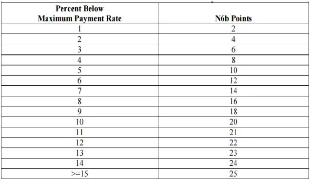
Environmental Benefits Index Estimate ... 47
Enrollment Decision ... 53 CRP Enrollment ... 55 Cropping ... 58 Cow-Calf ... 64 IV RESULTS ... 69 Test Assumptions ... 69 Output ... 73
vi
V CONCLUSIONS ... 80
REFERENCES ... 83
APPENDIX A ... 89
vii
LIST OF FIGURES
Figure Page
2.1 Acres Enrolled in the CRP in the US 1985-2013...………...13
2.2 Map of CRP Enrollment in Acreage per County – December 2014……...15
2.3 Disposition of Enrolled Acreage Under Hypothetical CRP Expiration Based on 2001 and 2002 Prices………...………...19
2.4 The Tradeoff between CRP Bid and EBI………...26
2.5 Average EBI Scores as of Sign-up 43; 2012………...28
4.1 CDF Comparison Enterprise Options Considered in the Decision Aid...74
4.2 Stoplight Comparison of 12 Enterprise Options Considered in the CRP Decision Aid ………...………...75
4.3 Stochastic Efficiency with Respect to a Function Analysis of 12 Enterprise Options Considered in the CRP Decision Aid ...………...77
viii
LIST OF TABLES
Table Page
2.1 Top Five Conservation Practices Installed on CRP Acres
(Current as of July 2014)………...10
2.2 CRP Payment Description Under Each Signup………...11
2.3 EBI Categories and Their Values..………...25
2.4 Soil Losses Under Various Crop Rotation and Tillage Practices………...32
2.5 Returns to Quail Hunting Within the CRP………...…...39
3.1 Conversion of Original Enterprise to CRP………...56
3.2 Penalty Calculator………...58
3.3 Cropland Establishment Budget………...62
3.4 Well and Associated Pump Budget………...64
3.5 Cow-Calf Budget...………...66
3.6 Cow-Calf Conversion Budget………...67
4.1 EBI/Bid Comparison Table………...72
4.2 Stochastic Dominance with Respect to a Function Analysis of 12 Enterprise Options Considered in the CRP Decision Aid ...……...76
4.3 Comparison of Enterprise Values Considered in the CRP Decision Aid………...78
1 CHAPTER I INTRODUCTION
The Conservation Reserve Program was established by the Food Security Act of 1985, with the primary purpose of preventing damage to highly erodible soils, made worse by intensified farming practices. Since its inception, the CRP has grown to
become the largest federal, private-land retirement program in the United States (Stubbs, 2014) with an approximately $2 billion annual budget.
At the end of 2014, approximately 24.2 million acres were enrolled in the CRP (FSA Monthly Summary, Dec 2014), with 77 percent of these acres being General Sign-up land, enrolled through a competitive bid process, and the other 23 percent being enrolled under Continuous Sign-up, targeting the specific needs of states and special goals of the federal government.
Since its inception, the CRP has grown to target much more than simply erodible soil. The CRP Annual Summary and Enrollment Statistics for FY 2012 estimates that runoff of nitrogen and phosphorus were decreased by 95 percent and 86 percent, respectively, compared to runoff levels had the CRP not been implemented. CRP reduces water pollution, and reduces hypoxic zones, particularly in the Gulf of Mexico.
The annual CRP report also estimates that there are approximately 2 million additional ducks/year added to the flock due to improved nesting provided by the CRP in the Prairie Pothole Region. In addition, the endangered sage grouse and lesser prairie
2
chicken have both seen an increase in numbers since the establishment of the CRP. Also, bobwhite quail density in upland buffers, a CRP management cover crops are 70-72 percent greater than on cropped land, and estimates show that a 4 percent increase in CRP land in a region can increase ring-neck pheasant numbers by as much as 22 percent.
CRP land reduces greenhouse gas emission levels. Estimates indicate that CRP land has removed 49 million tons of CO2 from the atmosphere. The reduction comes through the reduction of fuel use and nutrient runoff from fertilizer application, as well as CRP land itself serving as a carbon sink. The aggregate benefits of CRP equate to an estimated decrease of 9.6 million cars on the road (Conservation Reserve Program Annual Summary and Enrollment Statistics, 2012).
On top of all of these environmental benefits, the CRP has reduced “surplus” crops and boosted crop prices, provided stable income to landowners and producers, and bolstered regional economies through hunting and recreation. But CRP enrollment has also prevented more land from being planted when crop prices were record high.
The Agricultural Act of 2014 mandates a reduction in the enrollment cap from 32 million acres to 24 million acres by 2018. The cap reduction coupled with the higher than average commodity prices makes the decision of whether or not to reenroll land into the CRP a very difficult decision for producers with expiring land. Expiring lands will equal almost 2 million acres in the year 2015 alone, and approximately 7.1 million acres over the life of the farm bill (Conservation Reserve Program Statistics).
3
This research develops a computer based decision aid that incorporates all major aspects of the decision when considering enrollment in the CRP, to be used by
landowners and producers. These considerations include eligibility, the Environmental Benefits Index (EBI), the producers bid level, and evaluation of practice options within the CRP and options outside the CRP.
The goals of this research are to produce a computer web based decision aid, as described above, with specific emphasis on a few key output variables. These include a probability of acceptance measure, the Net Present Value of all options available to the landowner/manager, and a measure of what that landowner’s/manager’s optimal bid is.
4 CHAPTER II
REVIEW OF LITERATURE History of the CRP
The history of land retirement programs in the United States dates to the 1930’s, but they did not begin with the goal of preserving sensitive land. The 1930’s were an era of financial hardship for most American’s, and in particular, for those who lived in rural areas. Not only was the Great Depression at its peak, but the Dust Bowl was in full swing in the plains. According to “History and Outlook for Farm Bill Conservation Programs,” by Cain and Lovejoy 2005, in the 1930’s approximately one in four
Americans lived on farms, and an even greater percentage had incomes tied directly, or indirectly to farming. Yields were poor, and rural incomes showed it, dropping 52 percent from 1929 to 1933 (Cain and Lovejoy 2004). Poverty, along with other major concerns regarding agriculture led President Roosevelt’s Secretary of Agriculture, Henry A. Wallace, to produce the first “Farm Bill”, called “The Agricultural Adjustment Act (AAA)”.
The administration sought a way to support farmer incomes without using direct payments, as money being handed directly to individuals would have been politically impossible, and this led to the first real wave of land retirement. The AAA created a parity price for farmers. It guaranteed that, as long as you participated in voluntary production reduction programs, including acreage set-asides, the price you received would not fall below a set level based on parity to the 1910-1914 period. This program was not to last, as it was funded by a tax levied on processing of the commodities; a tax
5
that was eventually passed on to consumers. “In 1936 this tax was declared
unconstitutional on the grounds that Congress had passed a tax that was beneficial to one segment of the nation – the farmer – while causing detriment to everyone else.” (Cain and Lovejoy 2004)
Congress’ ruling led to the first real push towards large-scale conservation
programs. Before the finalization of the Supreme Court case, Wallace developed the Soil Conservation Act (SCA) of 1935. This method of getting cash to producers wasn’t challenged, and became the most significant method of support and surplus reduction in the 1936 Farm Bill. Unfortunately, Wallace’s SCA did not work as expected, and the cause was partly of his own doing. A huge supporter of science in agriculture, Wallace also supplied government funding for science and technology to advance the farming industry. This funding, which enhanced yields, led to significant slippage. Slippage can be described as a smaller reduction in production than expected from removing a certain amount of acres from production. In fact, due to the new tech and focused production on reduced acres, surpluses increased significantly following the 1936 Farm Bill.
Technology driven production gains exceeded the production of acres idled.
A few other adjustments were made to conservation initiatives prior to 1950, but due to the war-time economy and the need for more food production, focus shifted away from acreage controls for the majority of the 1940’s. Focus returned to conservation in 1956 with the passing of the Agricultural Act of 1956, which created the Soil Bank. The purpose of the Soil Bank was to, “[D]eal with the stifling effects of erosion that
6
threatened the welfare of every American and disrupted markets and commerce on the whole” (Can and Lovejoy 2004). The Soil Bank was made up of two programs, the Acreage Reserve Program and, in its first real iteration, the Conservation Reserve
Program. “The conservation reserve program called for a three-year contract wherein the government would pay for land improvements that increased soil, water, forestry, and wildlife quality if the farmer would agree not to harvest or graze contracted land” (Cain and Lovejoy 2004). The Soil Bank resulted in some unintended consequences that would affect future land retirement programs. The act devastated rural economies focused on agricultural processing and farming. Vast amounts of land were removed from
production in concentrated areas, effectively killing the processing industries that depended on through-put from the agricultural industry. This led to the 25 percent limit on acreage enrollment in a single county, which will be discussed later in the paper.
The 1980’s were the first time that conservation concerns began for the sole sake of conservation itself, without the explicit inclusion of price or supply control. The Food Security Act of 1985 was the first to have a conservation title, and it included the
creation of the Conservation Reserve Program as its own program, and the creation of Conservation Compliance. The first Conservation Reserve Program signup aimed at enrolling 40-45 million acres of highly erodible land, and was managed strictly on the goals of preventing erosion. This act included a provision allowing no more than 25 percent of acres in a county to be enrolled, to protect rural economies. Conservation compliance put regulations on land conversion and other practices in order for farmers to participate in farm programs.
7
The Conservation Reserve Program has undergone changes to its structure since 1985, but the overall idea has remained largely the same. In the Food, Agriculture, Conservation, and Trade Act of 1990, CRP saw a refocusing to include benefits to water, and created the first version of the Environmental Benefits Index (EBI). According to, “Conservation Reserve Program: Annual Summary and Enrollment Statistics FY 2012,” the EBI was later amended in the Federal Agriculture Improvement and Reform Act of 1996 to include emphasis on wildlife benefits equal to those gained by water and reduced soil erosion. The 1996 farm bill also led to the creation of the first continuous CRP sign ups. Continuous sign ups target specific state environmental issues and focus on aligning successes at the state level with the overall federal program. The Farm Security and Rural Investment Act of 2002 saw the creation of the, 4-of-6 previous year cropping rule, included provisions for non-emergency harvesting of CRP land, and expanded the Farmable Wetlands Program, enacted the year before, to all 48 contiguous states. Finally, in the Food, Conservation, and Energy Act of 2008, the acreage cap was decreased to 32 million acres.
The Agricultural Act of 2014 saw few significant changes to the CRP, mostly related to severe droughts occurring in Texas and California, and severe flooding in the Midwest. The first notable change was that emergency haying/grazing on CRP was now allowed with reduced or no penalty. In, “Conservation Reserve Program (CRP): Status and Issues,” Megan Stubbs of the Economic Research Service says that use of CRP land forage due to drought or flood, seasonal use of vegetative buffer practices, and grazing for a beginning farmer/rancher will be allowed with no penalty. However, managed
8
harvesting, commercial use, grazing for invasive species, routine grazing, and wind turbine establishment on land in the CRP will all be penalized 25 percent of their annual payment/acre. Many of these provisions came from the 2014 elimination of the
Grassland Reserve Program. The 2014 farm bill included a provision allowing early non-penalty termination of CRP contracts if the land has been enrolled for over five years, and is not considered “environmentally sensitive”. Lastly, in a continuing trend, the 2014 Farm Bill decreased the acreage cap of the CRP from 32 million to 24 million acres by 2018.
Operation of the CRP
The description of the CRP on the USDA Farm Service Agency website is, “In exchange for a yearly rental payment, farmers enrolled in the program agree to remove environmentally sensitive land from agricultural production and plant species that will improve environmental health and quality.” In reality, the program is much more
focused and intensive than this simple description leads one to believe, and has multiple initiatives working to specifically address the health of the environment, while balancing the needs of producers.
The CRP is administered by the Farm Service Administration (FSA) with support from other governmental agencies, primarily the Natural Resource Conservation Service (NRCS), and is funded by the Commodity Credit Corporation (CCC). It is the largest federal/private land retirement program, and widely considered to be one of the most successful.
9
The first consideration when looking at the CRP is determining what land is eligible. The first condition actually applies to the producer themselves. In order for a producer to be deemed ‘eligible’ for CRP they, “…must be an owner, operator, or tenant of the land for at least 12 months prior to the close of the CRP sign-up period, and show control of the land for the duration of the contract” (Stubbs 2014). There are special considerations that can get around this rule, but in general, it applies to all producers. The basic idea is to prevent people from buying land specifically for CRP enrollment.
Considerations for land eligibility are more extensive. In general, the land must be:
Highly erodible
Marginal pasture land
Grasslands in areas that could provide habitat for ecologically significant plant and animal populations if maintained/returned to grassland
Land to be enrolled in a riparian buffer
Each of these eligibility criteria have specific caveats that apply to them, ensuring that the land is used to its highest environmental potential, but in general, land must meet one of the above criteria in order to be eligible for enrollment. It is important to note that land is enrolled in one type of CRP ‘practice’ which is implemented via a plan created in conjunction with the farmer and FSA. The top five CRP practices are listed in Table 2.1. The established practice is voluntary, unless the specific ‘initiative’ a producer is
10
There are two ways to ‘opt in’ to the CRP. The first is through the general sign-up. The general sign-up is the largest portion of the CRP, and accounts for 19.7 million acres, or 77 percent of all land enrolled in CRP (Stubbs 2014). It operates on a
competitive bid process, whereby farmers submit a bid to the FSA and, based on their bid and environmental factors, the FSA either accepts or rejects their enrollment. General enrollment occurs during set time periods, and the next period begins on December 1, 2015, and ends February 26, 2016.
The second way to enroll land in the CRP is to work through the continuous sign-up. Continuous sign-ups are non-competitive and target the most environmentally sensitive land under specific needs of the state. These sign-ups include special signing and enrollment incentives to encourage participation. Continuous sign-ups account for 23 percent of CRP enrollment, or approximately 5.75 million acres. The largest two ‘initiatives’ under this sign-up are the Conservation Reserve Enhancement Program (CREP), and the Farmable Wetlands Program (FWP). These two initiatives account for 1.6 million acres of CRP enrollment.
11
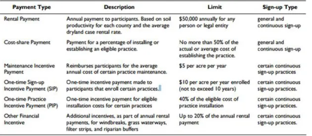
Table 2.2 is a detailed description of how payments work for each sign-up and initiative.
CRP payments to participants are based on a few factors that are discussed in detail later in this review, however, it is important to note that the payments cannot exceed the Maximum Acceptable Rental Rate (MARR), which is based on a calculation of the county average rental rate, taken from the National Agricultural Statistics Service, and takes in to consideration the soil productivity.
CRP is not in a sense ‘binding’ for the duration of the contract, as there are provisions for removing your land from the program. These provisions allow for the removal of land with some financial penalties. First, upon removal of land from the program, it is necessary to repay all financial incentives and one time payments in full,
12
with interest, and second, 25 percent of the rental payments received must be returned to the government.
Taxes on CRP payments are a timely issue. In October 2014, Morehouse v. Commissioner of the Internal Revenue was decided by the United States Court of Appeals, Eighth Circuit. In 1994, Morehouse inherited a large amount of land in South Dakota, and in 1997, after renting out a portion of the land to producers, and maintaining a portion in existing CRP contracts, chose to enroll another portion in the CRP. In an excerpt from the Decision on the case the circuit judge states:
Morehouse received CRP payments of $37,872 in both 2006 and 2007. The Morehouses timely filed tax return forms for both years and identified their occupations as “self-employed.” On Schedules E of their tax returns, the Morehouses listed the CRP payments for both years as “rents received,” and thus the CRP payments were not taxed as self-employment income. On October 14, 2010, the Internal Revenue Service
Commissioner (Commissioner) mailed to the Morehouses a notice of deficiency for 2006 and 2007. The notice stated the CRP payments should have been reported as income on a Schedule F, Profit or Loss From Farming, and were thus unreported self-employment income, which should have been taxed.
The Morehouses petitioned the Tax Court, which upheld the Commissioner’s claim, and the Morehouses in turn appealed the decision of the Tax Court. Eventually, the United States Court of Appeals, Eighth Circuit overturned the ruling based on the fact that, “…2006 and 2007 CRP payments were “considered paid [by the government] for the use [and occupancy] of [Morehouse’s] property” and thus constituted rentals from real estate fully within the meaning of § 1402(a)(1).” (Morehouse v. Commissioner, 2014) This means there are two methods of taxation for CRP revenue. If you are an active producer, revenue is subject to the 15.3 percent self-employment tax, however if you are a ‘non-farmer’ with land enrolled in the CRP, the money is not subject to the tax.
13 CRP Acreage
CRP is impacted by a myriad of forces, and can be significantly changed following upturns or downturns in prices, large environmental changes, or government program adjustments. Figure 2.1 shows the annual enrollment by acres from the CRPs inception to 2013. Note that in 2013 CRP acreage was the lowest it has been since pre-1990.
The most recent downturn in CRP enrollment follows a significant increase in commodity prices that began in late 2006. The upturn in commodity prices can be attributed to the aggressive increases in the Renewable Fuel Standard’s (RFS) volume requirements from 9 billion gallons in 2008 to 36 billion gallons by 2022 (H.R. 6, 2007), the sudden onset of drought in the Midwest and Texas during the 2010s, and higher
14
production costs. Higher production costs and drought cut corn supplies while the RFS rapidly boosted demand for corn for ethanol production. Higher crop prices, especially corn, meant there was less incentive for farmers to keep their land out of production if CRP rental rates remained the same. Even though, as we will later postulate, biofuel commodities are not the most commonly replaced by CRP acreage, an increase in price would lead producers to attempt biofuel commodity production on more marginal, i.e. CRP qualified land.
It should be noted that from 2008 to 2014 rental rates have, in fact, increased. According to data taken from the “Conservation Reserve Program Statistics” page of the FSA website, in 2008 the national average rental rate for cropland was $85.50/acre, while in 2014 that rate had increased to $141/acre. In a less significant, yet similar, trend the national average rental rate for pastureland went from $10.50/acre in 2008 to
$12.00/acre in 2014. While this is an increase, it is unknown if it was simply not enough to retain producers whose land might be highly productive, or if other factors kept them from the CRP.
CRP land is concentrated in a few large areas. The heaviest concentrations are generally located east of the Rocky Mountain range and west of the Mississippi river, however lesser concentrations of CRP are found in all 48 of the lower states except for Arizona. Figure 2.2 contains the CRP enrollment as of 2014, based on the concentration of acres in a county.
15
The highest concentration of acreage enrolled in the CRP occurs in the lower great plains encompassing areas in Texas, Oklahoma, Kansas, and Colorado, the Prairie Pothole Region, encompassing portions of Montana, North Dakota, South Dakota, and Minnesota, and portions of Iowa, Illinois, and Missouri.
Economics of the CRP
There are many economic factors to take into consideration when studying the CRP. In, “The Influence of Rising Commodity Prices on the CRP,” Hellerstein and Malcolm (2011) used a ‘Likely to Bid’ model to study the impact of rising commodity prices on CRP acreage and bid pricing. They simulated, at the national level, three
16
scenarios under which commodity crop prices stayed at their established baseline (prices in 2005), a medium level of prices (prices in 2007), and one in which the prices
remained at significantly high 2008 prices. They also tested two levels of Soil Rental Rate, the maximum level of allowable bids. The metrics they used to frame the study were differences in offered acres, average EBI scores (not including the cost factor of EBI), lost agricultural production through CRP enrollment, rental payments on an aggregate and per acre level, and regional distribution of acres. Their results indicated that higher crop prices were significant determinants of CRP bid prices. “[C]ommodity price changes influence not only the amount but the quality of lands offered: their agricultural productivity, environmental benefits, and geographic location” (Hellerstein & Malcolm, 2011).
Hellerstein and Malcolm’s findings for their baseline scenario indicate that 51.1 million acres would be offered into CRP. In the medium price (2007 levels) they used two different Soil Rental Rates. These rates were the 2007 SRR, and a SRR increased by 60 percent. With the 2007 SRR and the increased prices, the offered acres dropped to 28.8 million. With the increased SRR, offered acres went back towards the baseline scenario, reaching 45 million acres. Their results when conducting the high level price scenario, with an SRR increased by 120 percent from the baseline were similar to the increased SRR findings of the 2007 price level study.
SRR increases could help to combat price increases in commodities, and
17
model also gives an explanation as to why CRP acreage has decreased, despite increases in SRRs. Hellerstein and Malcolm did not have a, “…straightforward [method] to predict what rental rates would be under different commodity price regimes,” so they simply chose the 60 percent and 120 percent across the board increases. “Actual CRP rental rates increased by… 20 percent between 2008 and 2010.” (Hellerstein and
Malcolm, 2011) This provides insight as to why their predictions did not materialize, as the increase in payments was substantially less than the increases assumed in the study.
Changes in crop prices not only impact quantity of land enrolled in CRP, but also its locale and EBI scores. Hellerstein and Malcolm estimate that if prices stayed at 2007 levels, the costs of the program would double. Hellerstein and Malcolm also postulate that while this empirical analysis has held mostly true, variances in their results could be a result of the popularity of the program itself. Essentially, the popularity of the CRP program might mean that token increases in rental rates may keep producers in the program, even if it doesn’t explicitly meet their best financial interest. Overall,
Hellerstein and Malcolm find that, “Higher crop prices, as observed in summer 2008… are likely to sway some landowners in favor of agricultural production over
conservation,” and that, “[C]ommodity price changes influence not only the amount but the quality of lands offered[.]”
Sullivan et al. (2002), forecast the use of land were it to leave CRP. They first determined what factors influence the land use choice. Three factors; the type of cover used when the land is in CRP, the profitability of the possible uses, and the aspirations of
18
the owner, including age, wealth, and the tenure of CRP enrollment effected future land use. In an effort to simplify the study, aspirations of the owner were assumed away, and the type of CRP cover and the profitability of future uses were analyzed.
Sullivan et al. assumed that all CRP contracts were suddenly eliminated and used the Likely-to-Bid model developed by the Economic Research Service (ERS) to develop the probability that land will switch from CRP to another use. They based their data on 2001 prices and pre-2002 programs. They found that, when ending the CRP
immediately, 51 percent of CRP land would return to cropland, with the highest concentrations of this occurring in areas the authors named, the Northern Plains Crescent, which encompasses parts of Montana, North and South Dakota, and Wisconsin, the Southern Plains Ellipse, which includes portions of eastern Colorado, western Kansas, western Oklahoma, and the Texas Panhandle, and the Southwestern Corn Belt, which includes northern Missouri, southern Iowa, and eastern Illinois. The national average of 51percent is lower than found in previous studies, but they assume this could be due to the lack of personal information, or to the inclusion of new
assumptions on land rigidity as a good. Figure 2.3 contains an ERS estimate of what would happen to lands under the assumption that the CRP suddenly expired.
19
Increasing population pressure, along with a demand for higher standards of living in the developing world, is driving a need for more food, and therefore more places to grow it. In, “Is America Running out of Farmland?” Gottlieb addresses this concern by studying historical trends in population growth and land use.
20
Gottlieb discusses the dire predictions of a 1981 study that claims there is need for approximately 77 million acres of additional farmland to keep up with population growth. The fallacy of this argument is that it suffers from the Malthusian problem. The study assumed a straight line in both population growth and food supply growth,
although is technology may be actually increasing yields on the same amount of land. Even with the worst-case ‘straight-line’ scenario, the farmland ‘cap’ would not be reached until, at the earliest 2051, but with some estimates ranging all the way to the year 4000 (Gottlieb). The result is that the urban sprawl problem, and the loss of production land is not a ‘real’ problem.
Another issue that Gottlieb focuses on that is pertinent to the study of the CRP, is that market forces, along with technology will continue to provide adequate farmland. What this means is that, as the prices for commodities rise, as discussed previously, land will move away from uses like conservation towards production, as government
subsidies are unable to keep up with the market price of commodities. Gottlieb points out that the problem of farmland loss cannot be looked at as an aggregate, because transportation costs become an issue. With farmland in New Jersey cited as rapidly decreasing, the cost of transporting food to that region will go up, as the distance from food increases. This may, Gottlieb theorizes, drive local parcels that are enrolled in uses, such as CRP, out of those programs and in to production, as their returns would be higher on the market, and still less expensive than transporting commodities over long distances.
21
In, “Agricultural Land Values and Rents Under the CRP,” Shoemaker theorized that CRP might increase land values over time. The formula used to evaluate this claim was simple:
Impact on Farm Income = CRP Pmt. – Cover Establishment – Loss from Decreased Production
Shoemaker (1989) found that, with the CRP functioning as an annuity, the value has been bid-up by farmers and landowners treating enrolled land the same way they would treat a bond. Shoemaker stated that, “The direct effect of the CRP on eligible land depends on the excess beyond the minimum incentive required to induce participation in the program,” and “…that excess will be capitalized in to the program.” The research has interesting implications regarding farmer bids. According to the Shoemaker, “[T]here is a certain asymmetry of information regarding land quality.” In essence, the land owner knows a substantially greater deal about their land and its value than the government. This asymmetry of information allows farmers to gain ‘economic rents’. CRP rent is also a certain return vs. an uncertain farming return. During the first four sign ups, Shoemaker documented the behavior of farmers ‘bidding up’ their prices. “During the initial sign-up the average rental rates were lower than the bid caps in all regions. By the fourth sign-up, average contract rates approached or equaled the bid caps for all regions.” (Shoemaker, 1989) Farmers who wait to bid in to a program could discover their bid caps. The bid caps are now published and widely known, however it
22
does show that farmer bidding patters do not attempt to put less valuable land at a lower price, but always push the limit of the bid cap or Maximum Acceptable Rental Rate.
Jacobs, Thurman, and Marra (2011) discuss bidding practices in, “How Farmers Bid into the CRP: An Empirical Analysis of CRP Offers Data”. They discuss the fact that proposed rental rates are given negative weight in the EBI, and that the rental rate is what farmers base their bid on, as well as the EBI being roughly equal to a landowners probability of acceptance. According to Jacobs et al. producers face two problems when bidding. They have uncertainty about government actions and uncertainty about
competing bids on nearby acreage. The authors develop an equation that estimates the level at which a bid must be accepted:
𝑟 + 𝑏(𝑁) > 𝜋
where r is the bid, b(N) are other benefits assumed to be increased in future farming, social benefits, and unquantifiable “open space” enjoyment, and π is the returns to farming. The data came from signup data in the 16th, 18th, and 20th sign ups in the Prairie Pothole Region.
The authors found that bids are clearly conditioned on the Maximum SRR. They also found that changes in bids are not perfectly correlated. A $1.00 increase in the Maximum SRR only increased average bids by $.05 to $.55. This varied slightly by locale, as, landowners in Iowa and, to a lesser degree, Minnesota perceive (correctly) that they are penalized in the EBI cost scoring for being high rent enrollments which leads them to bid well below their maximum rental rate in an attempt to increase their
23
probability of acceptance. The opposite case holds for landowners in low rent areas (Jacobs et al., 2011). Also, the authors found that a landowner with a high EBI score will increase their bid by more than a landowner with a lower EBI score, if both gain one additional EBI point. This greater increase on high EBI scores is less likely to hurt the high EBI’s chance of acceptance, whereas it will likely keep a lower EBI score out of the program.
Williams et al. (2009) examined producer level concerns when considering the decision of whether or not to enroll in CRP, by conducting an empirical analysis to show the significance of incorporating risk when making the CRP choice. Multiple cited articles by the authors recommend leaving land idle at least one year after taking it out of the CRP to significantly increase yields. To incorporate risk, the authors conducted a static analysis and a stochastic analysis of several different production methods on sorghum-fallow and wheat-fallow rotations on an experiment station in Tribune, Kansas. The static study resulted in a substantial increase in income under the reduced till or no till methods over CRP. The stochastic study incorporates a producer’s general risk aversion, and found that, while conventional tilling has the highest returns to production, CRP has higher returns than any production methods. The authors determine that a risk averse/risk neutral producer will choose CRP due to their entire cumulative distribution function being positive under CRP, while under production, negative returns occurred. CRP was preferred to cropping for all producers when accounting for Absolute Risk Aversion Coefficient (ARAC) of greater than 0.04. Williams et al. work supported
24
incorporating risk when considering the economic CRP decision is important, as a large amount of CRP land is ‘marginal’ and financial losses occur frequently.
Feng, Hennessy, and Du (2013) argue that crop insurance should be considered when calculating the cost portion of the EBI, as high concentrations of CRP occur in areas of marginal land, where crop insurance premiums are high. The potential savings by not having to continue subsidizing those premiums are significant, and if included in the EBI, areas with high premiums could have more competitive bids. This could effectively change the geography of the CRP.
On a study of 12 counties in Southwest North Dakota, Bangsund, Hodur Leistritz, and Nudell (2011) conducted an analysis of the economic implications to an entire region from the reduction of CRP acreage. The authors found that, a reduction in CRP acreage, was correlated with significantly lower permit hunting returns, and that regional hunting related expenditures (i.e. hotel rooms, restaurant income) decreased. The authors point out that as CRP acreage decreases, there is typically a documented accompanying decrease in wildlife numbers. They hypothesize that the number of hunters and their spending decreases with fewer CRP acres. There are implications of ‘game-theory’ complications in the study, as the authors point out that, even if a farmer keeps his land enrolled in CRP, overall regional habitat loss will decrease the amount of wildlife, and therefore it is likely that fee-hunting revenues for an individual producer will decrease.
25 Environmental Benefits Index
The Environmental Benefits Index (EBI) has become an integral part of the CRP since it’s development in 1990. It was developed to compare the conservation benefits that different offered lands provide. Heimlich (2002) details the structure of the EBI. There are several components of the EBI in CRP. Table 2.3 contains the points given to each EBI consideration.
Following the measurement of the EBI benefits, the government creates a national standard EBI. Typically, lands that meet this national standard are considered acceptable for enrollment, contingent on their bid, while parcels that do not meet this
26
EBI are not usually accepted. The most recent standard EBI equaled a score of 209. (Stubbs, 2014) Once the environmental EBI is calculated, the government factors in the cost, and an important thing to consider is the fact that while the acreage of the program is capped, the costs are not. The government sets a Maximum Acceptable Rental Rate (MARR), which is essentially truncates the distribution of CRP bidders. Those with acceptable EBIs and rental bids below the MARR are accepted. The easiest way to envision the EBI is a type of balance (Figure 2.4), with costs on one side and
environmental considerations on the other. As your bid, accompanied by cost-sharing commitments from the government get ‘heavier’, your EBI must go up, and as your environmental benefits get ‘heavier’, you can place a higher bid.
The EBI is constantly in flux, and changes based on the needs of the current conservation attitudes, and political pressure. “The EBI was not meant to be a rigid index, but to be adjusted and improved depending on the progress of sign-ups, perceived deficiencies, and/or changed priorities” (Ribaudo et al., 2001). The EBI is often lauded
27
as a strong example of compromise in the political/conservation spectrum. “The EBI was not developed solely by scientists seeking to maximize the potential benefits from the CRP, but by a combination of program administrators, physical scientists, social scientists, and politicians trying to meet the demands of diverse consumer groups, the needs of farmers, and the realities of implementing a massive conservation program” (Ribaudo et al., 2001).
Figure 2.5 contains the average EBI score of land enrolled in the CRP as of the 43rd sign-up in 2012. As you can see, EBI scores tend to be concentrated in specific areas. These include the previously mentioned Southern Great Plains, the Northern Plains Crescent, the Southwestern Corn Belt, and the Deep South, although they all likely have differing environmental benefits.
28
Soil Fertility Considerations of the CRP
Depending on its use, land can function as a major carbon ‘sink.’ Along with nitrogen, these elements are essential for the healthy development of crops, and contribute to growth in yields. Loss of these nutrients creates the necessity for fertilization and therefore increases costs of production. Therefore, it is important to study whether or not CRP or different types of production are healthier for the soil.
Reeder, Schuman, and Bowman (1998) discuss the loss of Carbon (C) and Nitrogen (N) in the Central Great Plains. They began by testing land on seventeen
29
experiment stations with dryland cropping histories extending back from 40-60 years. They found that, compared to land that had been in its natural state for that period, C and N had decreased by 42 percent and 36 percent, respectively. They theorized that this was caused by exposure to erosion, reduced additions from organic matter, and enhanced soil organic matter (SOM) decomposition through depth mixing, temperature change, and aeration. One major question they hoped to address was the question of rate of decrease; do the levels of C and N decrease rapidly and stay low? Their estimates of achieving steady state ranged from 30-90 years.
In order to answer these questions, the authors selected two plots in Wisconsin (controlled for water erosion through selection of a level site), and applied treatments to each plot. One plot was a sandy loam soil, and the other was a clay loam soil. The treatments applied consisted of: native left in native, native land converted to cropping, cropped land left in cropping, and cropped land converted to native.
While fields left in their original states functioned as controls, with C and N remaining essentially unchanged, the results on the converted parcels were significantly different. There was a rapid decline in the levels of C and N on the native land converted to cropping, with the levels dropping in just 6 years, to the level of the cropped land that had been in production for 60+ years. This indicates that there is a rapid decrease in soil nutrients, and that they hit a steady state early after conversion. There was also a drastic change in soil nutrients on land that was converted from cropping to native state. After just 6 years in a managed CRP state, the land had reached levels of C and N greater than
30
that of land that had never been put in production in the first place. There was a small disparity between the types of soil, with sandy loam doing better than clay loam, but the results were the same overall.
Burke, Lauenroth, and Coffin (1995) studied organic matter to determine if, “…abandoned fields recover total soil organic matter, active soil matter, and N
availability after 53 years [of non-cropping, following decades of cropping]” (Burke et al., 1995). They theorized that tillage/cropping decreases SOM because these practices increase output of SOM and also decrease residual plant replenishment.
The authors used 12 sites in the Pawnee National Grasslands in northeast
Colorado, that they termed ‘abandoned’ fields. These fields had been cropped until 1942 and left idle until the study period in 1995. At five of their sites there was nearby
cropland they used as controls. Three sites were chosen from the Pawnee National Grasslands for immediate C and N testing, with their samples being refrigerated and sent to lab. The method of testing was soil core extraction with test depths of 0-5 in. and 5-10 in. below the surface.
“Microbial biomass C and N were significantly higher on both native and abandoned fields than on cultivated fields. However, there were no significant
differences between native and abandoned treatments with respect to microbial biomass for either microsite or depth.” (Burke et al., 1995) These findings support a large body of literature that says that cultivated land typically has 30-40 percent less C and N than native/abandoned land. Addressing this issue is important for land managers who are
31
considering taking land out of production or enrolling in the Conservation Reserve Program.
A key issue to address is the attempt to retain as much of the benefits gained from the CRP program as possible after the rejection of a parcels bid, or the choice to remove that parcel from the program. A key benefit to try to maintain is the soil retained from prevented erosion. Panuska, Good, and Wolkowski address this issue in,
“Converting CRP Land to Corn: Minimizing Soil Loss.” They use a SNAP (Soil Nutrient Application Planner)-Plus nutrient management software to evaluate the sediment loss from different farming methods. This program incorporates NRCS’s Revised Universal Soil Loss Equation (RUSLE2), and their data was taken from multiple fields with two differing slope ranges; 6-12 percent and 12-20 percent. Their results are found in Table 2.4, with the gray bars representing averages and the black lines representing actual observances.
32
The authors found that soil erodability and slope both significantly impact soil loss, and they compared the results to ‘tolerable’ soil loss, which is equal to the rate of soil formation. If the amount of soil loss is greater than the tolerable amount, there will be long term damage to the soil. Their suggestions following these comparisons are that, to prevent degradation, erodible, sloped land should be enrolled in CRP, and when planting corn, no-till or minimal-till is highly recommended, as is rotation, and the use of no-till cover crops for corn-silage are beneficial to the soil. It should be noted that corn is not the most common crop replaced by CRP in the Great Plains, which holds the highest
33
enrollment of CRP, but in the Southwest Corn Belt it is very common, and these results are likely transferrable to land that is commonly used to grow wheat, cotton, or sorghum.
Hunting and Wildlife on the CRP
A key difference in this study’s decision aid will be the inclusion of hunting benefits to landowners. Wildlife considerations account for a large portion of the EBI, and should also be considered when making choices on whether or not to retain land in the CRP or to convert back to cropland.
In, “Estimating the Response of Ring-Necked Pheasants (Phasianus Colchicus) to the CRP,” Nielson et al. attempt to determine whether or not Ring-Necked Pheasants (Pheasants) will be impacted by a change in the amount of CRP acreage enrolled in a given area. They point out that, due to their adaptability to differing habitats, pheasants should benefit from most types of CRP cover, and that in past literature an increase in CRP acreage typically increased the number of pheasants.
The study uses the Breeding Bird Survey (BBS) and data from the Farm Service Agency (FSA) to estimate whether or not CRP acreage will have an impact on pheasant population. The BBS methodology is simple; a driver and a spotter drive through different locales and stop for 3 minutes at pre-designated locations to count the number of birds seen or heard. This study took in to account all 4615 bird counts conducted within a year, and used the sum of pheasants along a route as an index of abundance. The study developed a set of ‘buffer’ zones. These zones had radiuses of 400 meters, 700 meters, and 1000 meters, and the percentages of CRP and other land types in each
34
buffer were used as predictor variables. These buffers were established based on the daily range of a pheasant’s movement. The study was conducted in two regions in the northwestern United States.
The final results find a positive relationship between pheasant numbers and routes with increased CRP acreage. An increase in CRP acreage by 4 percent correlated to an approximate 22 percent increase in the pheasant count, and as these results were similar across such a large range, the authors deem the information to be widely applicable and reliable.
With wildlife being a potential source of income during and post-CRP,
Geaumont, Vlaminck, Schauer, and Sedivec (2007) studied the number of pheasant on land that was recently removed from the CRP. The authors posit that managing post-CRP land for agriculture and environmental outputs can be beneficial environmentally and economically.
The authors selected two study sites that were 640 acres each that had, until recently, been CRP land. The plots were each split and given different treatments that included grazing by 33-45 cows, haying, idling, and cropping. The pheasant nests were found by ‘dragging’, or hooking a chain up between two vehicles and driving across a field every two weeks. When a bird ‘flushed’ they searched for the nest near that point and made a count.
The authors found that substantially more pheasant nested in the seasonal grazing plots and idled land, to the point that the cropping and haying results were
35
inconsequential. The authors believe this proves the need for maintaining areas of permanent cover, if pheasant production is a desired outcome. They also theorized that no more than 50 percent ‘disappearance’ of grazing lands would be sufficient for pheasant nesting.
The ring-necked pheasant is not the only species that is impacted by the CRP. The Prairie Pothole Region (PPR), or as it is sometimes called, “The Duck Factory,” is a region in the northern United States in which five of the most common species of ducks nest. The PPR was, at one point, covered in glacial formations that, as they receded, left huge ‘potholes’ that later filled with water and became millions of ponds that now make a prime nesting area for duck recruitment.
Reynolds, Shaffer, Renner, Newton, and Batt (2001) describe the CRP programs long term effects on the duck population in the critical area of the PPR. Between 1992 and 1995, the authors evaluated the success of duck nesting in fields composed of various types of CRP cover. The genesis of this study was the hope that due to increased conservation land through the CRP, the number of ducks would be increasing from their dismal levels, which were at their lowest levels in 1992 since 1955, when the counting of waterfowl species began. The evaluation of nesting success is important, as increased nesting success is directly correlated with increased duck numbers. The objective of the study was to estimate the average Daily Survival Rates (DSR) in CRP cover and
compare that with pre-CRP numbers, and to compare duck recruitment in CRP with a predictive model evaluating the situation if the land had never been converted to CRP.
36
The authors monitored 335 plots in the PPR, which were classified by cover type, and conducted annual surveys of those plots for breeding pairs. They then used
regression-ratio analysis to estimate the number of breeding pairs. One hundred thirty-eight of these plots included over 16.2 hectares of CRP land, which was a
pre-established measure for evaluation. These plots were the sites of nest counting.
Nest success and recruitment in CRP were 46 percent and 30 percent higher, respectively, than land without a presence of CRP. The authors noted that due to the presence of such a high quantity of CRP in the region, some of which were near control i.e. cropped fields, those controls may have been impacted. However, this does mean that the results, if anything, would increase. The authors found that CRP nest rates were as good as Wetland Reserve Program (WRP) nesting rates, and both were substantially better than predicted. The authors estimate this increase in nesting success and
recruitment adds 2.7 million ducks per year to the population.
The authors theorize that CRP may increase the success and recruitment of ducks for several reasons. The first is that an increase in grass provides increased cover for nesting and reduces predator contact with nests, and that the increased availability of other prey animals such as other birds, voles, and mice, which increase with the presence of CRP acreage, may decrease the need for predation by foxes on duck nests.
Nesting ducks are sometimes found in groupings or ‘hot spots’ and that several of these were found in CRP land. This could mean that ducks do prefer the cover of CRP managed land to even natural state land. While this is good during the presence of a
37
large amount of CRP, it does provide a potential explanation for the drastic drop in population after the initiation of the Soil Bank program. The authors hypothesize that, if ducks concentrate in CRP, and there is little CRP acreage, that there will be a over-nesting in CRP fields, which not only means adults may have to travel further for forage, leaving the nest unattended, but that predators have easier access to a large amount of nests at one time, making population decline intensify due to intensified nest failure. These explanations show that, if increased duck population is a goal of a landowner or a regional economy, enrollment in the CRP is a very viable option.
Once again addressing the possibility of wildlife management for post-CRP land, however this time with ducks, Geaumont, Sebesta, Sedivec, and Schauer (2007) tested multiple plots for duck populations. They theorized that, much like the case of the ring-necked pheasant, land exiting the CRP could be managed for agriculture and
environmental outputs in such a way that would provide profit for the producer both environmentally and economically. The study was conducted in the PPR region.
The methods were the same as the authors’ previous pheasant study. Two 640 acre sights were chosen, each having recently exited the CRP. The plots were split into different practices including grazing by 33-45 cows, haying, idling, and cropping. The duck nests were found by ‘dragging’ for birds, and searching for the nests when a bird had ‘flushed’. The authors do note that, due to the increased mobility of ducks, these results may be slightly less reliable than those of the pheasant study.
38
The authors found notable nesting concentrations by mallards, gadwalls, pintails, and teal, four of the five major species that nest in the PPR. The authors found that, while pheasant had limited nesting in cropped and hayed land, ducks avoided these areas entirely. They found zero nesting sites for any species in these plots. The authors found that their nesting rates were higher than any found in any other literature. The authors theorize that this was likely due to the presence of cattle, which discouraged the presence of any of the small predators that typically prey on ducks and duck nests. This, once again, supports the hypothesis that management in a CRP cover can realize rents from both agriculture outputs and hunting/environmental outputs.
In an attempt to prove that hunting on CRP land is a viable economic option, Williams and Mjelde (1994) authored a study entitled, “Conducting a Financial Analysis of Quail Huting within the CRP”, which establishes several practices and compares them to land idled in the CRP.
Under the study, the authors established three scenarios under which hunting could be compared to no hunting. Scenario One included amenities to guests such as accommodations and meals, along with pen raised birds. Scenario Two provides amenities to guests, but develops a wild population on CRP land. Scenario Three is a typical hunting lease on CRP land with an established wild population. Under their study they took budget items from the Texas regional average obtained from Texas AgriLife Extension Service, Texas Parks and Wildlife, the National Rifle Association, local appraisal districts, and the Texas Department of Agriculture. The authors assumed that
39
half of the establishment costs of the enterprise were shared under government funding, that there was no debt prior to the beginning of the enterprise, and that there was no borrowing.
The study results, simplified to fit this study of CRP are presented in table 2.5.
.
As you can see from the results, the best scenario, in terms of Net Present Value (NPV) is Scenario 1, netting over $40,000 more over the 10 year life of the analysis than the next-best scenario, Scenario 3. The authors note that economies of scale could change these results, and that assumed management practices within each scenario could be adjusted. While this study is slightly dated, (1994) it does prove the need for
evaluating hunting options in conjunction with operating CRP land.
Finally, in, “Wildlife Considerations in the Management of CRP Lands,” an appendix to a report published by the Texas Parks and Wildlife Department, the authors point out that, if habitat improvement is the goal, it should be noted that the same kind of CRP cover does not always work for all game species.
40
Under considerations for big game, the document specifically addresses the needs of mule deer, white tail deer, and pronghorn antelope, the major large species that are found on CRP land. The report states that these species will benefit from planned grazing and burning, as this helps with cover establishment and health. This cover provides ideal fawning conditions and escape cover from coyotes, the biggest threat to fawn populations. However, while the establishment of low brush is good for both deer species, it does not provide benefits for pronghorn, which are ideally suited to massive open range. The report does note that if CRP is established near cropping practices, the establishment of legumes or forbs will decrease the damage done to those cropped areas by these big game animals.
When planning for game birds, the considerations are as widely varied as the birds themselves. The specific birds identified by the report as inhabiting CRP are quail, pheasant, prairie chicken, and turkey. In planning for any of these birds, a planned burning or grazing will increase forb production which will increase insect production providing two types of food for these birds. It is also considered beneficial to hay, as long as it is after July 15, the end of the primary nesting season for most upland birds, and strategic places, like fencerows, are left alone.
When specifically targeting pheasant, it is advised to plant smaller tracts,
specifically fencerows in brush, as this can provide ideal habitat for the birds. The report mentions a common practice of the Texas Panhandle called cornering, which simple
41
means leaving the corners of the circle irrigation pivots idle. These corners provide ideal habitat for pheasant, and are frequented by hunters.
When planning for quail, there are two species to consider. Both operate in small tracts of CRP, but need separate cover types. Woody canopy cover and brush
establishment along fencerows will lead to more Northern Bobwhites, while less woody cover will lead to Scaled Quail.
When planning for turkey or prairie chickens on CRP land, the situation becomes more complex. The report says that these birds must have increased tracts of land
available in CRP, as they have a much larger range than the previously mentioned birds, and are more mobile on a daily basis. They must also have a more diverse habitat than quail or pheasant as their roosting habitats, escape cover, nesting, and feeding cover are not all the same.
When planning for waterfowl, such as ducks, geese, and cranes, it is
recommended that a 3:1 ratio of CRP upland buffers to playa basins is maintained. The Texas Panhandle, a region of the Southern Great Plains, is a major wintering area for ducks, geese, and Sandhill Cranes, as well as the Bald Eagle, and the retention of prescribed buffers with planned haying and grazing, along with legume inter-seeding is highly recommended.
This review of literature proves a few major points. The choice of whether or not a producer should leave their land in the CRP can have major financial decisions. There are a few major considerations to take when looking at that choice.
42
The first is to make sure the producer understands the function of the CRP and whether or not they, and their land, are eligible. This is a simple matter of informing the producer of their options and making sure they understand where their official
documentation can be found and returned to, as well as who they can contact about the program.
The second, more complex, area of this decision is incorporating producers EBIs and their bids. It is important to understand the balancing act of these two factors and how they are the key factors influencing a parcels probability of acceptance in the CRP.
The final important piece of the puzzle is ensuring the producer understands the options available. If they choose to stay, or enter, the CRP which practice will be the best choice for them financially and in terms of the health of their land? This must incorporate not only their budgets, but the variability of the fertility of their land. If they choose to exit the CRP, or their bid is not accepted, the producer needs to understand their options. These include, but are not limited to, commodity production, livestock production, continued conservation practices with no management, and continued conservation with wildlife in mind, either for hunting or not.
This study, and resulting thesis, develops a decision aid that accounts for all of these important components of the enrollment choice. By developing a model that accounts for eligibility, bidding, the EBI, and discounted net incomes from different options, a decision aid can help a producer make an informed decision that will impact their financial future, as well as the future of their land.
43 CHAPTER III METHODOLOGY Risk
Accurate economic modeling requires incorporating an element of risk. Risk is the part of a business model that cannot be controlled by the decision maker, also called the error term. Risk is particularly relevant to agriculture, which faces biological risk, price risk, weather risk, and risk associated with government policies. Ignoring risk in economic modeling can yield a point estimate, also called a deterministic estimate, however this method could under or overstate the risk of a particular investment.
Including stochastic values in an economic model incorporates an element of risk (Richardson, 2014). A stochastic model assumes two things that are essential to its operation. The first is that future risk is the same as historic risk, and the second is that while a variable may be unknown, its probability distribution is known. Stochastic models, and particularly Monte Carlo sampling, which is used in the Conservation Reserve Program Choice model, simulate risky variables a large number of times. This constructs a probability distribution of Key Output Variables (KOV) (Richardson, 2014) which can be used by a decision maker in evaluating the returns of a future investment. Richardson and Mapp (1976) use Net Present Value (NPV) as their key output variable, and indicate that this is an acceptable measure when evaluating investment decisions in small businesses, i.e. agriculture production.
44
As discussed previously, Monte Carlo simulation constructs probability distributions. There are two types of probability distributions, parametric and non-parametric (Richardson, 2014). A non-parametric distribution has known parameters, while a non-parametric distribution does not. The non-parametric distribution is used in cases when there are too few observations to find the required parameters for a parametric distribution. These parameters include mean and standard deviation, for a normal
distribution, and minimum and maximum values for a uniform distribution (Richardson, 2014). When these values are not known, an empirical distribution can be constructed using the sorted values of the available data and the probabilities of each of those values.
Richardson and Mapp (1976) lay out the steps for developing a simulation model connected to an investment decision. “The first step in developing a stochastic model for investment analysis is identification of critical variables…” (Richardson & Mapp, 1976). The next step is to develop probability distributions for those key variables thought to be stochastic. Next, links must be formed between stochastic variables, and fixed, or known variables that will influence the eventual outcome of the investment. Finally, these variables must be connected to accounting relationships associated with the proposed investment, and linked to the Key Output Variables (KOVs) (Richardson & Mapp 1976).
While simulation yields a more accurate prediction of an investments return by including risk, it is ultimately up to the decision maker, not the model, to act on that investment. When facing this choice, a decision maker’s attitude towards risk becomes important. Nicholson and Snyder (2012) describe decision makers as one of three risk
45
types; risk-loving, risk-neutral, or risk-averse, under the assumption that all three types are attempting to maximize utility.
Methods of Ranking Risky Alternatives
After the construction of a simulation model that includes risk, the decision maker must choose their option. Several simulation outputs constructed by Simetar, the software used in this research, can assist producers in these decisions.
The first method of evaluating multiple options is the cumulative distribution function (CDF). A CDF displays all possible outcomes for each option within the simulation, with the X axis representing an individual KOV’s value associated with the Y axis’ probability, which ranges from 0-1. This method’s major limitation is that the CDFs for each option often cross (Richardson, 2014). Under ideal circumstances, the decision maker would take the investment option whose CDF falls the furthest to the right, however, things become more complicated when the CDFs of two options cross, and it is often the case that more than two cross at different points.
Incorporating a decision maker’s utility function in ranking scenarios can impose a tighter restriction on risk aversion. This can be done using stochastic dominance with respect to a function (SDRF). A decision maker’s utility is bounded by a lower risk aversion coefficient and an upper risk aversion coefficient (LRAC and URAC
respectively) (Richardson, 2014). Each alternative is calculated at both the LRAC and URAC, and if the same choice is preferred at both levels, then the preferred alternative is the ‘efficient set’.
46
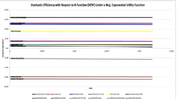
In 2004, Hardaker et al. developed a second method of ranking alternatives incorporating risk called stochastic efficiency with respect to a function (SERF). Like SDRF, SERF ranks risky alternatives over a specified range of risk preferences, in terms of certainty equivalences. Hardaker et al. According to Richardson (2014), SERF has the advantage of comparing multiple scenarios while SDRF can only compare pairwise combinations. SERF has two possible outcomes. When the certainty equivalent of an option is greater than the certainty equivalent of another option, that option with the greater certainty equivalent is preferred. The second option is that, when two options have an equal certainty equivalent, the decision maker will be indifferent between the two.
A final useful method of ranking risky alternatives is a stoplight chart ranking. This visual method of ranking evaluates probabilities of realizing favorable outcomes and displays them on a stacked bar chart. Outcomes that are deemed favorable are colored green, outcomes that are deemed unfavorable are colored red, and outcomes falling between the two thresholds, or cautionary results, are colored yellow. An
advantage of the stoplight ranking method is that it allows the decision maker to set their own threshold of ‘favorable’ and ‘unfavorable’, by selecting a lower cut-off value and an upper cut-off value. The idea of ranking scenarios based on probabilities was described by Richardson and Mapp (1976), and the stoplight method of presentation was presented by Richardson (2014).