Higher and More Stable Returns from Whole Cottonseed: An Examination of Utilization and Price Risk Management in Texas

HIGHER AND MORE STABLE RETURNS FROM WHOLE COTTONSEED: AN EXAMINATION OF UTILIZATION AND PRICE RISK MANAGEMENT IN TEXAS

A Thesis by

WESLEY SCOTT REGMUND

Submitted to the Office of Graduate and Professional Studies of Texas A&M University

in partial fulfillment of the requirements for the degree of MASTER OF SCIENCE

Chair of Committee, David P. Anderson Co-Chair of Committee, John R. C. Robinson Committee Member, John L. Park

Head of Department, C. Parr Rosson III

December 2016

Major Subject: Agricultural Economics

ii ABSTRACT

Price variability is a potential source of risk in the market for whole cottonseed. Conventional risk management practices for similar commodities consist of longer term storage, forward contracting, and hedging using futures markets as a means to combat unfavorable price movements. However, no futures market currently exists for whole cottonseed, limiting users and growers in their marketing planning and approaches for risk reduction. The purpose of this study is to examine cottonseed supply and usage patterns within Texas and to analyze the feasibility of price risk management strategies by cross hedging cash cottonseed with soybean and soybean meal futures.

Results from a survey disseminated to Texas cotton gins gave credibility to the idea that finding an alternative method to managing price risk would be economically beneficial. The relationship between cash and futures prices is significant enough to warrant further investigation and hedge ratios allowing for the proper risk coverage for a seller of seed are estimated. Additionally, a measurement of hedge effectiveness is considered and results in cross hedges using either soybean or soybean meal contracts that reasonably reduce risk when compared to an unhedged position. Practical testing from a seller’s perspective using historical data produced outcomes that showed that net effective prices from cross hedging are typically higher than unhedged cash prices over the considered time period. Though past performance is not an indicator of future

outcomes, this presents an additional potential outlet for cotton gins to market cottonseed aside from the traditional methods, and possibly improve their financial position and

iii

profitability. The strategies analyzed will conceivably allow growers, gins, oil mills, and livestock feeders to reduce price risk and uncertainty and aid in financial decisions.

iv

ACKNOWLEDGEMENTS

I would like to thank my committee chairs, Dr. David Anderson and Dr. John Robinson, and my committee member, Dr. John Park, for their guidance and support throughout the course of this research.

Thanks also go to my friends and colleagues and the department faculty and staff for making my time at Texas A&M University a great experience. I also want to extend my gratitude to the Texas Cotton Ginners’ Association, which provided insight and direction for developing the survey instrument, and to all the Texas cotton gin managers who were willing to participate in the study.

v

TABLE OF CONTENTS

Page

CHAPTER I INTRODUCTION……… 1

CHAPTER II REVIEW OF LITERATURE……….. 8

CHAPTER III METHODOLOGY……….. 12

Gin Survey……… 12

Cross Hedging Market Identification………... 13

Optimal Hedge Ratio Determination……… 15

Historical Simulation of Cross Hedging Strategies………..17

CHAPTER IV RESULTS……….21

Gin Survey……… 21

Cross Hedging Market Identification ... 28

Optimal Hedge Ratio Determination……… 33

Hedge Effectiveness………. 34

Historical Simulation of Cross Hedging Strategies………..36

CHAPTER V SUMMARY AND CONCLUSION……….. 45

REFERENCES………. 47

APPENDIX A SURVEY INSTRUMENT………... 49

APPENDIX B DRYLAND COTTON BUDGET……… 53

APPENDIX C IRRIGATED COTTON BUDGET……….. 55

vi

LIST OF FIGURES

Page

Figure 1: Map of Planted Acres in Texas in 2015 (USDA NASS 2015)………...1

Figure 2: 2015 Estimated Revenue for South Plains Extension District 2 (Texas A&M AgriLife Extension 2015)………..2

Figure 3: Cottonseed Usage from 1994-2015………...….4

Figure 4: 2015 Estimated Dryland Ginning Costs for South Plains Extension District 2 (Texas A&M AgriLife Extension 2015)………...5

Figure 5: Location of Gins from Survey Responses………...21

Figure 6: Cottonseed Sales by Purchaser, South Texas Region, 2014………...22

Figure 7: Cottonseed Sales by Purchaser, West Texas Region, 2014………...23

Figure 8: Cottonseed Sales by Purchaser, Cooperative, 2014………....24

Figure 9: Cottonseed Sales by Purchaser, Independent, 2014………...…….24

Figure 10: Percentage of Cottonseed Sales by Month, South Texas, 2014………...….26

Figure 11: Percentage of Cottonseed Sales by Month, West Texas, 2014………...…..26

Figure 12: Percentage of Cottonseed Sales by Month, Statewide, 2014…………...27

Figure 13: W. Texas Cottonseed Cash Price vs. Nearby Futures Prices………...…...29

Figure 14: W. Texas Cottonseed Cash Price vs. Nearby Soybean and Soybean Meal Futures Prices………..………...31

Figure 15: Average Effective Net Price from Cross Hedging Using Soybeans…...…..42

Figure 16: Average Effective Net Prices from Cross Hedging Using Soybean Meal………43

vii

LIST OF TABLES

Page Table 1: Descriptive Statistics of Price Series and Basis Series

June 2007—December 2015…………..………...31 Table 2: Price Level Correlation Coefficients between Cottonseed and Exchange

Traded Commodities………...…...32 Table 3: Estimated Regression Parameters………....33 Table 4: 4 Month Pre-Harvest Cross Hedging Example Using Soybean Futures…...38 Table 5: July Storage Cross Hedging Example Using Soybean Meal Futures………..39 Table 6: Average Effective Price September-December 2007-2015…….…………....40

1 CHAPTER I INTRODUCTION

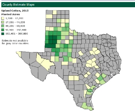
According the National Agricultural Statistics Service (USDA NASS), 4.5 million acres of upland cotton were harvested in the state of Texas in 2015, which produced 5.72 million bales. This places cotton as the leading cash crop in the largest producing state. Cotton is mostly grown in counties within the West Texas Panhandle and along the Gulf Coast as seen in Figure 1.

Figure 1: Map of Planted Acres in Texas in 2015 (USDA NASS 2015)

Generated from that harvest was 1.844 million tons of cottonseed valued at nearly $415 million, ranking it in the top seven crops grown within Texas in terms of

2

production value. Cottonseed is an important joint product of upland cotton production, where roughly 700 pounds of seed on average are produced from each 480-pound bale of cotton (Cotton Incorporated). The value of whole cottonseed is a significant factor in the overall economics of cotton production. Returns from whole cottonseed represent slightly below 20% of the estimated gross returns from total production in

Texas. Revenue estimates provided by the Texas A&M AgriLife Extension Service for 2015 in the South Plains District show this to be the case for both higher yielding irrigated acres and lower yielding dryland acres. Figure 2 shows the expected revenue table for a dryland producer in this region from the full example budget concerning costs and returns per acre, which can be found in Appendix B.

Figure 2: 2015 Estimated Dryland Revenue for South Plains Extension District 2 (Texas A&M AgriLife Extension 2015)

Four products that are derived from whole cottonseed are oil, meal, linters, and hulls. The oil and meal produced from crushing and further processing the kernel make up a large portion when determining the value of the overall seed. Meal is predominantly used for livestock feed, while the oil is almost entirely utilized in manufacturing salad dressings, cooking oils, and baking goods for human consumption. The linters, which are short fibers that cling to the seed, have some use in making paper currency and upholstery. However, they along with the hulls, which are the protective coating for the

3

kernel, mostly end up in livestock feed. Therefore, world markets for vegetable oils and feed ingredients have a substantial role in establishing cottonseed’s value (National Cottonseed Products Assoc.).

Whole cottonseed is a valuable ingredient in livestock rations, especially for dairy cattle. It is considered a complete supplement that offers a protein content of 23%, a fat (energy) content of 20%, and 24% crude fiber on a dry matter basis (Cotton

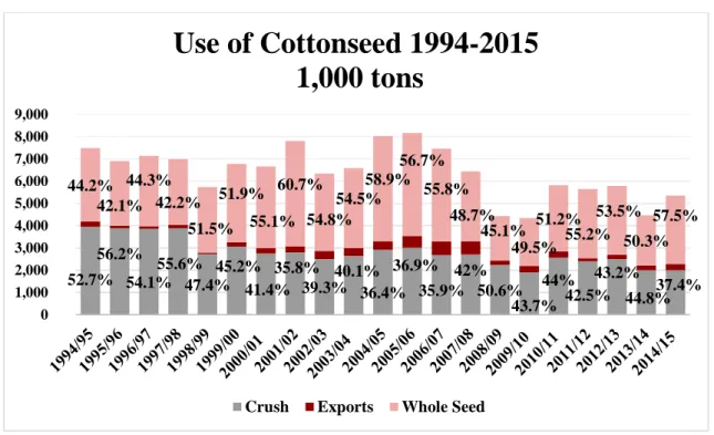
Incorporated). The high energy and protein stem from the kernel of the seed, while the fiber comes from short strands commonly referred to as linters that remain on the seed after the cotton lint is removed. Because of its use as a feedstuff, cottonseed competes with other ingredients such as corn, soybeans and soybean crush components, and other oilseeds. Cotton Incorporated describes one fourth of U.S. whole cottonseed as being sold directly from gins as livestock feed, and another quarter is distributed as livestock feed products after being processed by a cottonseed oil mill. Given the importance of the Texas livestock industry, it may be that the share of Texas whole cottonseed being fed to livestock is greater than the national average. Historically, a large portion of the seed was sent to mills and resulted in crush products. However, since the late 1990s a majority of seed has been kept whole mostly in the form of feed. Production and usage data provided by USDA NASS in Figure 3, estimates that in the 2014/15 marketing year roughly 58% of cottonseed remained whole compared to 37% being crushed and 5% being exported to world markets.

4

Figure 3: Cottonseed Usage from 1994-2015 (NASS, USDA 2015)

There is little available information on the seasonal marketing of Texas cottonseed. The value of Texas cottonseed has traditionally been applied to offset ginning costs and past swings in price occurred as a result of inadequate storage

capacities (Cotton Incorporated). Ginning expenses are typically the single largest cost for cotton producers and account for slightly below 20% of the total variable costs. This is exhibited in Figure 4, which is the variable cost table of a dryland operation in

Appendix B. Historical observations of Texas whole cottonseed price implies that most of the time the price will be within plus-or-minus $69 per ton around the average price of $290 per ton. This level of variation is enough to expose growers to occasional ginning cost increases.

52.7% 56.2% 54.1% 55.6% 47.4% 45.2% 41.4% 35.8% 39.3% 40.1% 36.4% 36.9% 35.9% 42% 50.6% 43.7% 44% 42.5% 43.2% 44.8%37.4% 44.2% 42.1% 44.3% 42.2% 51.5% 51.9% 55.1% 60.7% 54.8% 54.5% 58.9% 56.7% 55.8% 48.7% 45.1% 49.5% 51.2% 55.2% 53.5% 50.3% 57.5% 0 1,000 2,000 3,000 4,000 5,000 6,000 7,000 8,000 9,000

Use of Cottonseed 1994-2015

1,000 tons

5

Figure 4: 2015 Estimated Dryland Ginning Costs for South Plains Extension District 2 (Texas A&M AgriLife Extension 2015)

Stabilizing the value of whole cottonseed would have beneficial financial implications for Texas cotton producers. The significant decline in cotton lint prices in 2015 led to widespread financial losses for cotton producers. The 2014 Farm Bill eliminated cotton as a Title I commodity and implemented STAX, an insurance type program, instead of the ARC and PLC options used for other Title I commodities. A number of oilseed crops, primarily soybeans, have access to ARC and PLC. Cotton

6

producers viewed cottonseed as an oilseed crop and requested its inclusion in farm program support. However, this appeal came well after the passage of the farm bill and its implementation. The Secretary of Agriculture subsequently ruled that cottonseed is not designated as a covered oilseed, therefore keeping it ineligible for payments

provided by farm programs. This added uncertainty in managing price variation might also represent a significant risk to the financial position of gins, co-ops, livestock feeders, and other users.

Conventional risk management practices for other storable agricultural commodities consist of longer term storage, forward contracting, and using futures markets as a means to combat unfavorable price movements. However, special

considerations must be made for storing such products and no futures market currently exists for cottonseed. This limits users and growers in their marketing planning and risk reduction strategies. The purpose of this study is to identify and evaluate applicable cross hedging strategies for whole cottonseed in Texas. After an appropriate review of the literature (Chapter 2), this study involves the following: 1) collection of primary data on whole cottonseed utilization in Texas, 2) examination of commodities with

established futures markets to identify an appropriate cross hedging vehicle for West Texas whole cottonseed, 3) determination of optimal hedge ratios for selected cross hedging commodities, and 4) historical simulation and evaluation of applicable cross hedging strategies for whole cottonseed. The strategies analyzed will conceivably allow growers, gins, oil mills, and livestock feeders to reduce price risk and uncertainty and aid

7

in financial decisions. Although this study is primarily focused on markets within the state of Texas, the same methods can be used in other regions.

8 CHAPTER II

REVIEW OF LITERATURE

The agricultural economics literature does not generally contain many studies involving cottonseed, and those that do exist are mainly focused on examining its value in beef or dairy cattle feeding or uses of the oil or meal produced from further processing the seed. Coppock, Lanham, Horner (1987) and Myer (2009) discuss the high nutritional value of whole cottonseed in cattle feeding rations and how to maximize its benefits in the Southern states, where most of the nation’s cotton is grown. These researchers also address the issue of the toxic substance called gossypol, which is found when high levels of cottonseed are present in a ration. This toxin not only limits the amount of seed that can be fed to cattle, but also is a significant factor in hindering uses of whole cottonseed in non-ruminant and human consumption.

When addressing the reduction of price variability, hedging is a commonly used and effective risk management tool for agricultural producers and processors. This is typically accomplished through a direct hedge where one futures position offsets one cash position. However, in cases where physical commodities have no specific futures contract, such as cottonseed, Anderson and Danthine (1981) suggested that a cross hedge can be placed by taking a position in a related, although indirect, futures market. They also presented the concept that a correlation coefficient differing from zero indicates an appropriate cross hedging vehicle and that ratios of futures contracts can give optimal coverage for one’s cash position.

9

Following the path of Anderson and Danthine, Blake and Catlett (1984)

examined corn futures contracts as a means to hedge against price variations in United States and New Mexico spot alfalfa hay markets. After finding sufficient correlation between prices, they used multiple regression techniques to determine the optimal contract months for both pre-harvest and storage based hedges and the optimal ratio of coverage based on the Mid-America Exchange’s 1,000-bushel corn contract. Simulated routine cross hedges were performed using previous years’ data and showed that gross return per ton of hay increased compared to a non-hedged scenario.

Likewise, while evaluating the possibility of cross hedging rice bran and millfeed, Elam, Miller, and Holder (1986) discovered that a simple hedge using solely corn futures provided less risk in divergent net and target prices than without a hedge in place. They also discovered that risk associated with cross hedging using corn futures was not significantly different from when other futures contracts were included to implement a multiple cross hedging strategy.

In order to gain a better understanding of how effective these hedging strategies were for various products depending on the type of hedge being considered, Witt, Schroeder, and Hayenga (1987) suggested that the technique to properly estimate the hedge ratio varies. For a purely anticipatory hedge where the current cash price is irrelevant; the hedge ratio can appropriately be found by price level regression. If the current cash price is relevant, such as with storable goods, a price change model is more appropriate.

10

When determining how to best calculate the appropriate amount of the cash position to hedge in order to minimize the variance of terminal wealth, Lence, Kimle, and Hayenga (1993) examined a dynamic minimum variance hedge in their study that allows for an agent to adjust the positon of both the cash and futures in the hedge. Their estimations of a corn storage problem found that this dynamic hedge ratio is more practical and operational than other dynamic models, but gains in hedge effectiveness when compared to a simpler static minimum variance hedge ratio were negligible.

With grain by-products gaining prevalence within livestock feeding rations, Coffey, Anderson, and Parcell (2000) examined the possibilities of cross hedging corn gluten feed (CGF), hominy, and distiller’s dried grain (DDG) using corn futures and soybean meal futures as hedging vehicles. Their research concluded that while there was some correlation in price levels between the futures contracts and non-exchange traded products, the reduction in price risk did not outweigh the risk introduced by the hedge. Therefore, it is difficult to use cross hedging as a means to reduce risk associated with each by-product.

In similar fashion, Dahlgran (2000) examined cross hedging opportunities for outputs produced by the cottonseed milling process, such as meal, oil, and hulls. He discovered that a combination of contracts from various exchanges can be used to implement a sufficient hedge for the cottonseed “crush”. However, while this study was statistically significant in reducing risk, in application this example is uneconomical due

11

the cost and time associated with managing large positions in multiple contracts and exchanges.

Adding to the work of Dahlgran, Rahman, Turner, and Costa (2001) explored the feasibility of using soybean meal futures as a cross hedging vehicle for cash cottonseed meal. They found that cash cottonseed meal prices and soybean meal futures prices show a direct price movement relationship. They then provided examples of cross hedging using estimated hedge ratios and concluded that hedged net realized prices were generally higher than cash prices.

A common method for evaluating hedge effectiveness in all previous work was a comparison of R² values. Sanders and Manfredo (2004) claimed this is done with no attempt to determine if the results are statistically significant. They proposed a

methodology which determined whether or not the improved hedging performance of one contract compared to another is more meaningful. By using OLS regression of changes in cash prices on changes in futures prices, the residual basis risk can be determined. The correlation of basis risk between different contracts was then used to calculate the significance and weight given to each contract in reducing risk. They then illustrated this method by comparing two competing futures markets, choosing multiple cross hedges, and evaluating a proposed futures contract.

12 CHAPTER III METHODOLGY

Gin Survey

Because whole cottonseed market distribution information is not widely available, an on-line survey was created and disseminated to cotton gins throughout Texas. The purpose of the survey was to gain a better understanding of distribution and utilization patterns, and assess the risks associated with buying and selling cottonseed for gins, growers, and livestock feeders.

While developing the survey instrument, input was sought from members of the Texas Cotton Ginners’ Association. Initial versions were reviewed by the organization, and their feedback helped improve the direction and clarity of this study. The survey questions were modified to increase the likelihood of appropriate and useful responses. The survey instrument, which can be found in Appendix A, was targeted towards both cooperative and independently owned cotton gins across Texas. The final questionnaire was created using Qualtrics, a survey software that allows for online data collection. It was then distributed via email by the ginners’ association, which encouraged gins to participate in the study. The survey and a reminder was sent again 19 days after the original circulation to prompt additional responses. Responses were recorded within the Qualtrics system and were converted into an Excel file where they were aggregated and formatted for easier viewing. All respondents offered the location of their gins and its

13

governing structure, with a lone gin electing to not complete the remainder of the questions.

Cross Hedging Market Identification

With no current contract available for trade on any widely used commodities exchange, various grain and oilseed futures contracts were considered as candidates for cross hedging cottonseed cash prices at the gin or oil mill level. Possible cross hedging contracts evaluated included soybeans, soybean meal, soybean oil, and corn, all of which are traded at the Chicago Board of Trade, and act as substitutes for cottonseed as protein in livestock rations. Additionally, the canola contract offered by the Winnipeg

Commodity Exchange was considered as well as the cotton contract on the New York Mercantile Exchange. In order for cottonseed to be hedged effectively, there needs to be an adequate correlation between the cash and futures price series.

West Texas whole cottonseed price information came from Feed Ingredient Weekly published by Informa Economics and is comprised of weekly average prices in this region. Data were unavailable for a few weeks throughout the study period and this was corrected by averaging the prices of the previous and following week. The weekly average of the nearby futures contract settlement price for each examined commodity were provided by the Commodity Research Bureau beginning in June 2007 through the end of 2015. Each weekly average futures series was rolled to the next nearest contract one month prior to expiration to account for decreases in liquidity and trading volume.

14

This futures price information was then converted from its contract price per unit into United States dollars per ton ($/ton), the common price quotation for West Texas whole cottonseed. Correlations between the weekly cottonseed cash price and weekly near month futures prices of the aforementioned contracts were calculated using Microsoft Excel for the price level, price changes, and percent changes in price. Witt, Schroeder, and Hayenga (1986) determined that price change models are more appropriate for storable goods since the current price is relevant. While whole cottonseed can be considered a storable commodity, from a practical standpoint it is more perishable than other feed grains and has more limited and unique storage capabilities due to its bulky nature and tendency to retain moisture. Anecdotal evidence, which surfaced while developing the survey, suggested that only 20% of cooperative owned cotton gins in Texas had storage available for seed. Also, as a feedstuff, whole cottonseed is not

typically sold a great deal in advance. This suggests a more anticipatory hedging point of view may be necessary. In addition, many observed prices for cottonseed are similar from week to week. This causes numerous values of zero to occur from price changes suggesting that using price level data is most appropriate in this scenario as previous works propose, (Parcell, et al. (2008), and Brinker, et al. (2009)). Likewise, Myers and Thompson (1989) found that coefficients were only marginally better when first differences were used. The correlation coefficients were calculated using the complete weekly price series from June 2007 through December 2015. Shorter time periods were also considered as suggested by Costa and Turner (2003) as well as lagged prices to account for autocorrelation; however, increases in correlation using these methods were

15

varied and not significantly improved. Dickey-Fuller tests found futures prices to be stationary. Once proper correlation was established, basis risk introduced by the proposed hedge instruments was assessed. The basis is defined as the cash cottonseed price minus the price of the specified futures contract at a given time. The standard deviation of this basis series, or basis risk, can be compared to the standard deviation of the price series which forms the general price risk. The commodities were evaluated and contracts that showed less variation of the basis compared to overall price variation received further consideration in the study since this does not create greater total risk when a hedge is put in place.

Optimal Hedge Ratio Determination

A recurring issue for hedgers and traders is how to best select the appropriate number of contracts needed within the futures position to sufficiently cover one’s spot, or cash, position. Since a cottonseed contract does not exist and alternative commodities involve different factors that affect price movement, a perfect hedge cannot be achieved. The traditional benchmark in the hedging literature to estimate the optimal hedge ratio is to use the slope coefficient from a simple regression either on price levels or price changes. This is a static ratio of the futures position relative to the cash position to be hedged that minimizes the variance in total value for a risk adverse user. The Ordinary Least Squares (OLS) regression model for cash cottonseed and soybean meal futures prices can be shown as:

16

where 𝑊𝑇𝐶_𝑆 is the weekly West Texas cottonseed spot price, 𝑆𝐵𝑀_𝐹 is the weekly average soybean meal futures settlement price, and 𝜖 is simply the error term. The intercept term, 𝛽₀, represents the average difference between the cash cottonseed price and the soybean meal futures price. The slope coefficient or the optimal hedge ratio, 𝛽₁, indicates the typical cash price change associated with a one dollar price change in the futures. This method has been criticized for not recognizing time-varying distributions or cointegration between prices. It also is seen as imposing unrealistic restrictions on decision makers as it implies that neither the cash position nor the futures position can be revised or adjusted between the time the hedge is placed and the time it is lifted. Recent studies using time-varying and dynamic models to allow for the optimal hedge ratio to change over time have shown differences from that of static models; however, as shown by Lence, Kimle, and Hayenga (1993), McNew and Fackler (1994), as well as others, the gains in hedge effectiveness when compared to a static variance minimizing ratio are often insignificant. General acceptance of the OLS established ratio has occurred because it is relatively simple to empirically estimate and offers an easy to understand and practical tool while still providing reasonably accurate estimates.

Using this ratio, the equation to calculate the necessary number of contracts to offset a given amount of cottonseed to be hedged can be written as,

17

where 𝑁_𝐹 is the number of futures contracts, 𝑄_𝑐𝑠 is the amount of cottonseed (in tons) to be hedged, 𝑄𝐹 is the quantity associated with one futures contract converted into

tons for this scenario, and ℎ∗ represents the optimal hedge ratio.

Historical Simulation of Cross Hedging Strategies

After estimating the ideal number of contracts, empirical tests simulating cross hedging strategies were conducted to analyze returns by a cotton gin in both hedged and unhedged scenarios. Historical evaluation for finding net realized or effective prices for cross hedged commodities has been implemented in numerous studies previously conducted by Blake and Catlett (1984), Rahman, Turner, and Costa (2001), Parcell (2008), and many others. This practical application based on historical data is an

effective method for assessing the performance of a hedging strategy and the likelihood of improved returns for the user.

Simulated strategies in this study were explored from the viewpoint of a cotton gin or a seller of physical seed. Since the Texas cotton harvest begins in late August, gins naturally start receiving cottonseed from the ginning process at this time and sales of the seed to either oil mills or livestock feeders continues mostly from then through the end of December. Gins can employ either a pre-harvest based cross hedge or one that takes the limited time of storage into account. A pre-harvest cross hedge involves taking a short position in the futures market before the cotton harvest and then lifting that position as possession of the cottonseed occurs and selling takes place. To remove the hedge, the gin manger must buy back an equal number of future contracts to offset the

18

short position. Alternatively, in the event of storing and holding cottonseed before the sale date, a short position is taken in the nearest futures delivery month when the seed arrives and the hedge is maintained until the time of sale arises. In this situation, if the cottonseed remains in storage when the futures contract matures, the cross hedge is lifted and simply rolled forward into the next delivery month as necessary.

Both scenarios were tested using soybean and soybean meal contracts. The pre-harvest cross hedge was executed by placing the hedge four months prior to the expected sale date and then lifting the short position in the futures market once the physical seed was sold during the September through December time period. Four months prior to harvest was chosen as the time length because the gin is likely aware of the amount of cotton acres planted and can reasonably estimate the expected production and cottonseed volume. Analysis using this approach involved changing the date the hedge was

implemented as well as the date when spot market sales were performed so that they remain four months apart. Similarly, a cross hedge was assessed while taking storage into account by placing the hedge in the nearby futures on the first week of July and lifting it at the time of sale between the first week of September through the last week of December. In this scenario, the date the hedge was applied remained constant as the first week July, while the selling of cottonseed changed by a week over the four-month time period. Employing the hedge at this time allows the gin to assess their storage

capabilities and cotton yields more accurately just before harvest while still being able to protect against falling prices once possession of the seed takes place.

19

To calculate the effective net price received by the gin, the revenue from the sale of the cottonseed was added to any gain or loss associated with the futures transaction to determine the total revenue. This value divided by the amount of cottonseed sold results in the realized price received by the gin. This can be shown as:

Revenue from Cottonseed Spot Sale:

[3] 𝑅𝐶𝑆 = 𝑃𝐶𝑆 × 𝑄𝐶𝑆

where cottonseed revenue, 𝑅_𝐶𝑆, is equal to the price of cottonseed at the time of sale in the cash market, 𝑃_𝐶𝑆, multiplied by the amount of cottonseed sold in tons, 𝑄_𝐶𝑆.

Revenue from Futures Transaction:

[4] 𝑅_𝐹 = (𝐹𝑃₀− 𝐹𝑃₁) × 𝑁_𝐹× 𝑄_𝐹

where 𝐹𝑃0 represents the initial price of the futures contract when the short

position is executed. 𝐹𝑃₁ denotes the futures price when the hedge is lifted by taking a long position in the futures market at the time the physical cottonseed is sold. 𝑁_𝐹 is the number of contracts needed to cover the amount of cottonseed using the optimal hedge ratio, and 𝑄_𝐹 is the size of the futures contract in tons.

Effective Net Price:

[5] 𝐸𝑁𝑃 = (𝑅𝐶𝑆_𝑄+ 𝑅𝐹)

20

as stated previously, the combined revenue from selling cottonseed in the spot market, 𝑅_𝐶𝑆, and the profit or loss from the futures transaction, 𝑅_𝐹, determines the effective net price once it is divided by the quantity of cottonseed sold in tons, 𝑄_𝐶𝑆.

A cross hedge using this method is deemed successful and effective when a gain in the futures market occurs due to declining prices and concludes with a calculated net realized price that is greater than the cash price of unhedged whole cottonseed.

21 CHAPTER IV

RESULTS

Gin Survey

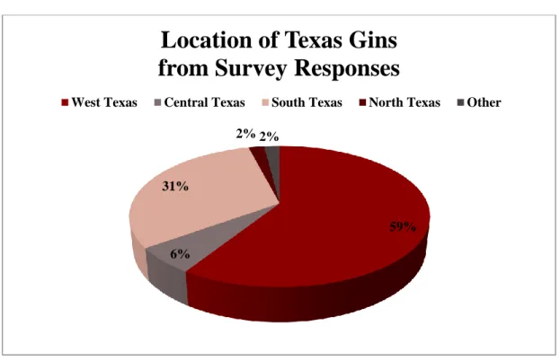
Of the 214 active gins surveyed across the state, 49 replied to questions about the location and governing structure of the gin, how much cottonseed the gin sold in 2014, the type of purchaser and method of sale, the time of year in which the seed is typically sold, and any price risk management strategies the gin may put into practice. Naturally, a large portion of the responding gins were located in the Panhandle and West Texas, as well as along the Gulf Coast in the southern part of the state. The geographical representation of responding gins can be seen in Figure 5.

Figure 5: Location of Gins from Survey Responses

59% 6%

31%

2% 2%

Location of Texas Gins

from Survey Responses

22

Gins, consisting of 59% with cooperative ownership and 41% independently owned distributed an average of approximately 12,000 tons of cottonseed per gin during 2014 to various users such as oil mills, dairies, and feedlots depending on their location. The ratio of cooperative and independent gins and the amount of seed sold per gin was similar in all regions. Figure 6 shows the percentage of seed sold to the different users in the South Texas region. A majority of the seed sold in this area goes to the local

cooperative oil mill, Valley Cooperative (VALCO), and a significant portion to the Archer Daniels Midland (ADM) oil mill.

Figure 6: Cottonseed Sales by Purchaser, South Texas Region, 2014

Likewise, the largest amount of seed in the West Texas area is sold to the regional cooperative oil mill, PYCO Industries (PYCO), exhibited in Figure 7. Dairies purchased larger quantities of whole seed in this area given cottonseed’s valuable impact

17.97% 55.70% 0.34% 4.64% 1.59% 12.95% 6.81% 0% 10% 20% 30% 40% 50% 60% 1

Cottonseed Sales by Purchaser

South Texas

2014

23

on milk quality and that a majority of the dairy production resides in this part of the state.

Figure 7: Cottonseed Sales by Purchaser, West Texas Region, 2014

Examining the purchasers of seed when comparing the governing structure of the gins showed different tendencies as well (Figures 8 & 9). Gins that operate as

cooperatives were, perhaps unsurprisingly, more likely to sell their seed to the primary cooperative oil mill in the region, VALCO in the South and PYCO in the West.

Alternatively, independently owned gins sold larger portions to other oil mills in the area, outside brokers, or directly as feed to dairies.

6.36% 44.26% 0.98% 1.09% 1.42% 11.39% 28.02% 6.49% 0% 10% 20% 30% 40% 50% 1

Cottonseed Sales by Purchaser

West Texas

2014

Oil Mill: ADM Oil Mill: PYCO Oil Mill: Other Feed Mill

24

Figure 8: Cottonseed Sales by Purchaser, Cooperative, 2014

Figure 9: Cottonseed Sales by Purchaser, Independent, 2014 6.95% 61.62% 1.29% 2.95% 2.24% 16.94% 7.89% 0% 10% 20% 30% 40% 50% 60% 70%

Cottonseed Sales by Purchaser

Cooperative

2014

Oil Mill: ADM Regional Oil Mill Oil Mill: Other Feedlot Dairy Broker Other

21.04% 12.80% 1.83% 2.02% 19.30% 39.59% 2.93% 0% 10% 20% 30% 40% 50% 60%

Cottonseed Sales by Purchaser

Independent

2014

25

Survey participants were given the option to comment on which brokers

purchased their seed or where the seed was sold if “Other” was selected. In most cases, the “Other” response resulted in the seed being sold as feed to local ranchers or to

farmers to use for future planting. Though it appears slightly more seed in these areas are being sent to oil mills compared to amounts suggested by Cotton Incorporated and the National Cottonseed Products Association (NCPA), the overall survey results on the buyers of whole cottonseed are similar to the usage data provided by USDA NASS.

The time of year when cottonseed sales took place also varied somewhat by region. Since planting and harvest of cotton occurs earlier in the southern portion of the state compared to the Texas Panhandle this was an expected result. This was relayed in timing of sales as southern gins began in August and were mostly complete by

December, represented in Figure 10. Northern gins, showcased in Figure 11, started selling more significant amounts in October, with November and December being the main months. Roughly 82% of all statewide seed was sold beginning in August until December, as seen in Figure 12.

26

Figure 10: Percentage of Cottonseed Sales by Month, South Texas, 2014

Figure 11: Percentage of Cottonseed Sales by Month, West Texas, 2014 0 10 20 30 40 50

Jan Feb Mar Apr May Jun Jul Aug Sep Oct Nov Dec

1.00 _{0.33 0.33 1.00 1.00 0.33 1.00} 27.60 42.07 17.87 6.87 1.93 %

Percentage of Cottonseed Sales by Month

South Texas 2014

Jan Feb Mar Apr May Jun Jul Aug Sep Oct Nov Dec

11.45

2.69 1.97 0.90 0.82 0.37 0.33 0.09 0.52

12.01

31.08 31.91

%

Percentage of Cottonseed Sales by Month

West Texas 2014

27

Figure 12: Percentage of Cottonseed Sales by Month, Statewide, 2014

Many respondents noted that there is a significant risk of fluctuating prices of cottonseed which influences their financial position. Storage of seed and forward

contracting were methods described to help mitigate this risk and take advantage of more favorable prices. Cross hedging was mentioned in discussions with gin members as a means to manage price volatility, but this strategy is not typically implemented. Comments received within the survey that stated that down-side price risk was not a major concern for some gins because oil mills bought their seed at contracted prices. Oil mills help shoulder the threat of changing prices with these common agreements.

Additionally, many remarks mentioned that producers of cotton face financial risk because the value of the cottonseed generally pays for the cost of ginning their cotton. A

0 5 10 15 20 25

Jan Feb Mar Apr May Jun Jul Aug Sep Oct Nov Dec

7.42 1.73 1.29 0.86 0.81 0.33 0.51 8.68 14.50 14.21 23.03 21.42 %

Percentage of Cottonseed Sales by Month

Statewide 2014

28

producer may receive a rebate if the price of cottonseed is greater than ginning costs; however, if the cost is greater, then the farmer must pay the difference. The results of the ginner survey show there has been a very limited study or application of hedging

strategies for whole cottonseed,andgave credibility to the idea that finding an

alternative method to manage price risk would be economically beneficial for not only gins in Texas, but for producers and users of cottonseed as well.

Cross Hedging Market Identification

Figure 13 shows the weekly average historical price series for West Texas cash cottonseed (W. Texas), and the near month weekly average futures contract prices for soybeans (SB), soybean meal (SM), soybean oil (SO), corn (C), and canola (CA). This visual representation indicates it is likely that there is considerable correlation between cash cottonseed prices and the prices of the exchange-traded commodities.

29

Figure 13: W. Texas Cottonseed Cash Price vs. Nearby Futures Prices

There was substantial volatility in these prices over the considered time period. A major boom in 2007 through 2008 led to prices increasing across almost all commodities to rarely seen before levels. This was driven by a combination of surprisingly tight supplies, growth in emerging countries, low interest rates, and a thriving biofuel industry subsidized by governments (Carter, Rausser, and Smith 2011). United States cotton prices nearly tripled from the middle of 2010 through the beginning of 2011 after the world’s largest and fourth largest producing countries, China and Pakistan respectively, experienced severe flooding that greatly reduced their yields. This combined with India, the world’s second largest producer, banning the export of cotton and strong global demand led to the dramatic price increase (Cancryn and Cui 2010). Also a significant drought during the summer of 2012 in the largest corn and soybean producing states in

$0 $200 $400 $600 $800 $1,000 $1,200 $1,400

Jun-07 Mar-08 Jan-09 Nov-09 Sep-10 Jul-11 May-12Mar-13 Dec-13 Oct-14 Aug-15

$

/t

o

n

W. Texas Cottonseed Cash Price vs. Nearby Futures Prices $/ton

June 2007 - December 2015

30

the Midwest United States caused prices for those crops to reach historical highs. These events had substantial impacts on the prices of crops and increased their range of movement.

Summary statistics providing the average and standard deviations of these prices can be seen in Table 1, which offers further insight into the comparison of movement and volatility of the price series. Possible explanations for the varying degrees of fluctuations in price could be differences in demand and use for these products after processing or the weather patterns in regions where the crops are typically grown. Corn is used in the manufacturing of ethanol which is a component of gasoline. For example, corn prices became more susceptible to changes in demand for fuel when government regulation of ethanol mandated its inclusion in gasoline. Additionally, canola is grown in regions, such as the Pacific Northwest, that experience less extreme weather conditions compared to the areas where cotton and cottonseed are produced leading to more

moderate changes in price from year to year. Furthermore, other crops, such as soybeans, are eligible to receive government support from farm programs and are more easily stored throughout the year leading to a more consistent supply and more stable prices.

31

Table 1: Descriptive Statistics of Price Series and Basis Series June 2007—December 2015 ($/ton) Cottonseed Soybean Soybean Meal Soybean Oil Corn Canola Cotton

Price Series Mean 292.89 396.47 353.96 873.81 178.34 585.33 1,611.56 St. Dev. 69.11 75.16 67.47 192.79 50.66 82.72 584.28 Price Risk Basis Series Mean (103.57) (61.07) (580.59) 114.55 (291.82) (1,318.34) St. Dev. 58.92* 53.48* 178.91 58.81 74.45 575.06 Basis Risk Note: The basis series is composed of the weekly cash cottonseed prices minus the futures prices from June 2007 to December 2015. * Indicates that basis risk is less than overall price risk of the commodity and lower than price deviations of cash cottonseed.

Soybeans and soybean meal appear to be most aligned with cottonseed price movement as shown in Figure 14 and Table 2.

Figure 14: W. Texas Cottonseed Cash Price vs. Nearby Soybean and Soybean Meal Futures Prices

$100 $200 $300 $400 $500 $600

Jun-07 Apr-08 Jan-09 Nov-09 Sep-10 Jul-11 May-12Mar-13 Jan-14 Oct-14 Aug-15

$

/to

n

W. Texas Cottonseed Cash Price vs. Nearby Soybean & Soybean Meal Futures Prices

$/ton

June 2007 - December 2015

32

Table 2: Price Level Correlation Coefficients between Cottonseed and Exchange Traded Commodities

Soybean Soybean Meal Soybean Oil Corn Canola Cotton

Cottonseed 0.67 0.69 0.37 0.55 0.52 0.19

Although a standard minimum correlation coefficient needed for effective

hedging is not established in previous works, values significantly differing from zero are deemed to be relevant (Anderson & Danthine 1981). The correlation between the cash cottonseed price and futures prices in this instance is slightly below the typical

coefficient values found by former studies examining cross hedging. Though most of these crops have a significant and similar role in the livestock feeding industry,

differences in price movement may be explained, as previously mentioned, by demand factors further along the production line or supply issues. Most notably, cotton has the lowest correlation coefficient suggesting that determinants of supply, such as harvested cotton acres, have less of an impact than demand influences associated with oilseed markets. Only soybean, soybean meal, corn, and canola futures have a correlation with whole cottonseed prices that exceeds 0.5 (Table 2). Further, Coffey Anderson, and Parcell (2000) show that assessing basis risk can also help in determining the

relationship needed for an effective hedge. As seen in Table 1, the basis risk associated with these contracts, aside from corn, is less than the price risk, warranting their

inclusion and additional exploration of cross hedging cottonseed. Further examination focused on soybean and soybean meal contracts, as they exhibited the highest correlation with cottonseed price (Table 2), have a lower basis risk compared to their price risk

33

(Table 1), and do not appear to introduce greater amounts of risk when a hedge is put in place.

When further assessing these two contracts, measuring the correlation of basis risk can help determine if a composite hedge provides greater risk reduction or if a single contract is an appropriate tool. Drawing on the principles suggested by Sanders and Manfredo (2004), the relatively high correlation of basis risk between soybean and soybean meal advises against the use of a combination of these contracts since no further benefits of diversification are included with the additional commodity.

Optimal Hedge Ratio Determination

Table 3: Estimated Regression Parameters1

Soybean Meal Soybean Intercept 42.12 49.66 Slope 0.709 0.614 R-Square 0.48 0.45 F-Ratio 412.25 361.10 Prob(F) 0.00 0.00 S.E. 0.035 0.032 T-Test 20.30 19.00

1 _{Durbin-Watson tests result in low values of 0.066 for soybeans and 0.086 for soybean meal indicating}

positive autocorrelation of their residuals is present. Though the estimators remain unbiased and

consistent, they are less efficient and the standard errors are likely smaller than their true values (Pindyck and Rubinfeld 1991). However, regressions using lagged variables to account for autocorrelation resulted in trivial differences in statistical values. Likewise, estimating with Generalized Least Squares (GLS) techniques produced the same values as OLS estimation. These results are similar to those found by Atanlogun, Edwin, and Afolabi (2014).

34

Shown in Table 3, slope coefficients produced for soybean and soybean meal contracts regressed on cash cottonseed at the price level are 0.614 and 0.709,

respectively. As previously mentioned, these values represent the optimal hedge ratio and indicate an average change in cash price when a dollar change in the price of futures occurs. If a gin needs to hedge 1,000 tons of cottonseed, then selling four soybean futures contracts (1,000/150 × 0.614 = 4.09) is needed to appropriately hedge the selling of the seed. A single soybean contract consists of 5,000 bushels or 150 tons. Since trading fractional contracts is not possible, rounding to the nearest integer is required when calculating the number of contracts. Similarly, if a seller were using the soybean meal contract, which equals 100 tons, as a cross hedging tool, then selling seven futures contracts becomes the requirement (1,000/100 × 0.709 = 7.09).

Hedge Effectiveness

In this case, the R² levels for soybean and soybean meal, seen in Table 3, are below the 80% explanatory value recommended by some previous studies of cross hedging effectiveness. However, it seems unreasonable to expect one competing commodity to have such a profound impact on cottonseed price movement given the wide ranging and differing factors that affect the crops. Additionally, as Sanders and Manfredo (2004) found, many of the previous studies that considered the high R² value as the standard for determining hedge effectiveness did so without defining the statistical significance of this value.

35

Wilson (1989) and Srinivasan (2011) concluded that a measure of hedge performance can be used to determine how well the spot price risk is reduced when a hedge is introduced. To do this, the variance from an optimally hedged portfolio is compared to the variance from an unhedged portfolio. The variances are simply:

[6] 𝑉𝐴𝑅𝑈𝑁𝐻𝐸𝐷𝐺𝐸𝐷 = 𝜎𝑆2

[7] 𝑉𝐴𝑅_{𝐻𝐸𝐷𝐺𝐸𝐷} = 𝜎_𝑠2(1 − 𝜌2)

where 𝜎_𝑠 is the standard deviation of the spot price and 𝜌 is the correlation coefficient between cash and futures prices. From this, the hedging effectiveness (HE) can be measured as the percentage reduction in variance that a hedged position creates contrasted with the variation from an unhedged position. This reduction can be

calculated as:

[8] 𝐻𝐸 = 1 −_𝑉𝐴𝑅𝑉𝐴𝑅𝐻𝐸𝐷𝐺𝐸𝐷

𝑈𝑁𝐻𝐸𝐷𝐺𝐸𝐷

The value produced from this equation can be interpreted as the average decrease in cash price risk that is realized when hedging takes place. A hedge that completely eliminates risks results in 𝐻𝐸 = 1, and implies a 100% reduction in variation.

Alternatively, risk reduction approaches 0% as HE falls to zero. The corresponding HE value using soybeans as hedging tool is 0.45. Applying a soybean meal cross hedge has a value of 0.48, indicating that either option is reasonably effective at reducing risk when compared to an unhedged situation.

36

Historical Simulation of Cross Hedging Strategies

In the first scenario examined, it is assumed that in the first week of May a cotton gin is aware of estimated cotton production from planted acres and can reasonably assess the amount of cottonseed as well. The gin manager anticipates the need to sell

cottonseed in the first week of September, four months away. Because the price of cottonseed might be lower at that time due to increasing supplies at harvest, the gin manager protects against downside risk by currently selling the appropriate number of contracts using either soybean or soybean meal futures. If the futures price declines, a gain is made on the short position and offsets a decline the cash price of cottonseed. On the other hand, a loss is incurred if the futures price rises. Once the gin takes possession and sells the seed in the spot market on the first week of September, the manager buys back the same number of futures contracts to lift the hedge. The loss or gain on the futures transaction can then be added to the value of the cottonseed sold and a net effective price received by the gin can be determined. A successful cross hedge is evaluated by its ability to capture gains from falling prices while minimizing variation and results in an effective net price that is greater than the unhedged cottonseed cash price.

For example, on the first week of May in 2014 the price of cottonseed in the West Texas cash market was $430 per ton. With the need to sell 1,000 tons of cottonseed at what the gin manager foresees as a possibly lower price at harvest, the manager sells four soybean future contracts at the Chicago Board of Trade which is currently trading at

37

$14.65 per bushel or $488.37 per ton. On the first week of September, the gin sells its new crop cottonseed at the now traded cash price of $287.50 per ton for total revenue of $287,500. Although the gin did not have ownership of the seed back in May, this

represents a $142.50 per ton decline in the spot price. At the same time, the manager lifts the hedge by buying four soybean futures contracts for $339.73 per ton. The futures transaction results in a gain of $148.64 per ton per contract, not including commission on trades, or a total payoff of $89,191($148.64 × 150 × 4). The total return of

$376,691($287,500 + $89,191) results in a net realized price the gin receives of $376.69 per ton. This net price is $89.19 per ton greater than what the gin would have collected by selling unhedged seed in the spot market. This example is shown in Table 4. The same calculations were made every week until the last week of December with the futures position taken four months before the sale date and lifted when the physical cottonseed was marketed. This strategy resulted in an effective net price received due to cross hedging that was greater than the unhedged cash price 69% of the time, over the same months in 2007 through 2015, with the average effective price being $289.36 per ton compared to $271.03 per ton in a no hedge scenario.

38

Table 4: 4 Month Pre-Harvest Cross Hedging Example Using Soybean Futures

Time Cash Futures

First week of May 2014

(Four Months Prior to Sale Date)

$430/ton Sell 4 soybean futures contracts @ $488.37/ton

First week of September 2014 Sell 1,000 tons of

cottonseed @ $287.50/ton

Buy 4 soybean futures contracts @ $339.73/ton Gain = $148.64/ton Revenue from selling cash cottonseed = $287.50 × 1,000 = $287,500

Profit from futures transaction = $148.64 × 150 × 4 = $89,191 Total revenue = $287,500 + 89,191 = $376,691

Net effective price = $376,691 ÷ 1,000 = $376.69/ton

Another approach was tested using a storage-like cross hedge that begins with the seller of seed taking a short position in the futures market on the first week of July regardless of the expected selling date. July was chosen as the naïve month to place the hedge because around this time a more accurate assessment of storage capacity and cotton yields leading up to harvest can be made. It also exhibited the highest and most frequent profit from the futures transaction of all months observed. The gin manager will then lift the hedge whenever the spot sale occurs. In this example, cottonseed is priced at $327.50 per ton and nearby soybean meal futures are trading at $350.93 per ton on the first week of July in 2015. Shorting seven soybean meal contracts is necessary for the gin to protect against a decline in price for 1,000 tons of cottonseed, as mentioned earlier using the optimal hedge ratio. As ginning begins and new crop cottonseed arrives in the warehouse, the gin manager decides to store the seed until the last week of December with the hope that cash prices will increase later in to or after harvest. Unfortunately, on

39

the last week of December when the physical cottonseed is sold, the spot price has fallen to $265.50 per ton; however, the soybean meal futures price has also declined by $76.60 per ton and is trading at $274.33 per ton. Once the futures position is reversed and the hedge is lifted, the transaction has a subsequent profit of $53,620 ($76.60 × 100 × 7), excluding the cost of commission. The cottonseed is sold to an oil mill or livestock feeder at this time for a total of $265,500 ($265.5 × 1,000). This combined with the gain in the futures results in a total return of $319,120 or an effective price of $319.12 per ton received by the gin, which exceeds the unhedged cash price by $53.62 per ton. These calculations can be seen in Table 5. Placing the hedge using soybean meal futures on the first week of July and lifting the position every week from the first week of September until the last week of December produced a higher realized price relative to an unhedged price by an average of $24.62 per ton. The better price experienced by the gin was a 67% occurrence from 2007 to 2015 with an average value of $295.65 per ton.

Table 5: July Storage Cross Hedging Example Using Soybean Meal Futures

Time Cash Futures

First week of July 2015 $327.50/ton Sell 7 soybean meal futures contract @ $350.93/ton Last week of December 2015 Sell 1,000 tons of

cottonseed @ $265.50/ton

Buy 7 soybean meal futures contracts @ $274.33/ton Gain = $76.60/ton Revenue from selling cash cottonseed = $265.50 × 1,000 = $265,500

Profit from futures transaction = $76.60 × 100 × 7 = $53,620 Total revenue = $265,500 + 53,620 = $319,120

40

The same test procedures were implemented for the pre-harvest scenario using soybean meal futures as the cross hedging vehicle and taking a short position four months prior to selling cottonseed. Additionally, soybean futures were assessed while taking storage into account by placing the hedge on the first week of July and lifting it at the time of sale beginning on the first week of September through the last week of December. Cash and effective net prices for the four different hedging scenarios were averaged over the 2007 to 2015 sample period and are reported in Table 6. The storage-like July placed hedge using soybean futures as the tool for cross hedging provided the highest returns and most consistent results over this time period.

Table 6. Average Effective Price September-December 2007-2015

Cash Cottonseed Soybean July Hedge Soybean 4 Mo. Hedge Soybean Meal July Hedge Soybean Meal 4 Mo. Hedge Average Net Price

($/ton) $271.03 $296.60 $289.36 $295.65 $289.06 % of time Hedged

Net Price > Cash Price

74% 69% 67% 63%

Avg. Amount Over

Cash Price $25.58 $18.81 $24.62 $18.51

Average Gain Over

Unhedged Price $50.14 $44.09 $51.44 $46.31

Max. Gain Over

Unhedged Price $161.94 $143.11 $135.29 $165.65

Average Loss Below

Unhedged Price $ (37.50) $ (36.49) $ (26.54) $ (29.65) Max. Loss Below

Unhedged Price $ (85.70) $ (73.33) $ (67.80) $ (77.05)

The effective net prices were averaged for both cross hedged scenarios and the unhedged approach concerning the different weeks examined between the first week of September and the end of December over the 2007 through 2015 sample period. The

41

differences between the strategies can been seen in Figure 15 for the hedges using the soybean contract and Figure 16 where soybean meal was the hedging vehicle. The prices over the observed weeks indicated that the storage-like hedge in July using either the soybean contract or the soybean meal contract will on average result in an effective net price that is greater than the effective net price found for both the unhedged scenario and the approach where the cross hedge is executed four months prior to selling in the cash market. As noted previously, there is the possibility of experiencing a loss, or a lower effective net price, as a consequence of hedging. This takes place in instances where price movement between futures and cash markets become dissimilar. Though these occurrences were observed less frequently with lower magnitudes using this historical data, the average and maximum amounts when hedged prices were lower than unhedged prices are reported in Table 6. The average and maximum values for gains when the hedged prices were higher being also represented. The threat of losses is notable from a financial risk standpoint because they signify occasions when margin requirements must

42

be met by the hedging gins. This has the ability to reduce operating funds and becomes a cash flow issue if the losses from short positions stretch over lengthy periods of time.

Figure 15: Average Effective Net Price from Cross Hedging Using Soybeans $240 $250 $260 $270 $280 $290 $300 $310 $320 $330

Sept. Oct. Nov. Dec.

$

/t

o

n

Average Effective Net Price Soybean Hedges September - December

2007-2015

43

Figure 16: Average Effective Net Prices from Cross Hedging Using Soybean Meal

Outlying years in 2007 and 2010 produced no weeks in which any hedges were profitable. This is presumably the result of highly uncharacteristic and unexpected movement in prices due worldwide factors mentioned earlier. Divergence of prices may also be affected by speculative forces in the futures markets. Additionally, the cost of trading in the form of brokerage commissions and margin requirements were taken into consideration; however, the varying amounts for these costs and their lack of any significant influence on the ultimate outcome resulted in their exclusion during calculations. Total commission costs would vary slightly between the scenarios as different hedging lengths were used requiring the need to roll contracts into the proper delivery month and different quantities of contracts were bought and sold depending on the cross hedging vehicle chosen. There would also be different margin requirements

$240 $250 $260 $270 $280 $290 $300 $310 $320 $330

Sept. Oct. Nov. Dec.

$

/t

o

n

Average Effective Net Price Soybean Meal Hedges September - December

2007-2015

44

associated with the separate exchange-traded commodities. When selecting the

appropriate strategy, if a hedger is not merely seeking the highest return but is concerned with cash flow and liquidity then these factors are important and will need to be

accounted for.

The conclusions of these strategies should be considered within the observed time period. These findings are representative of the historical data, and although past performance is not an indicator of future outcomes, the overall results tend to support that on average the probability of more consistent and higher gains outweigh the less frequent and less severe threat of lower realized prices through hedging concerning this time window.

45 CHAPTER V

SUMMARY AND CONCLUSION

Opportunities for research to build upon this study exist as it assumed that there are factors affecting cottonseed that do not necessarily have an impact on soybean or soybean meal prices. Outside influences such as government intervention in the form of farm program supports, demand for goods of processed commodities, and available global supply of competing crops have an effect on these prices. Protein and dairy markets may also have a growing impact on whole cottonseed price movement due to its increasing use as an ingredient in cattle feeding. Additionally, supply determinants may need further examination with respect to their effect on price movement of cottonseed. The dramatic increase in the price of cotton and its subsequent decline most likely had a substantial impact on the lack of correlation as cottonseed prices did not follow suit. However, as cotton prices are recently more stable, the variation between the prices has become more similar. This may require additional consideration to cotton as a cross hedging tool in the future.

Alternative hedging approaches should also be considered in future work.

Different hedging horizons and lengths can be explored and dynamic time-varying hedge ratios can be implemented for possibly more effective hedges. A gin also has the option of selling its cottonseed in the cash market and taking a long position in the futures market thereafter. This would allow the gin to take advantage of rising prices that were missed due to no longer having possession of the seed. When gins engage in forward

46

contracts with oil mills, this different kind of risk is introduced and can be managed by implementing this strategy. Hedges using options is also a common method that can be investigated. These derivatives may offer improved price risk reduction but have different cash flow considerations to take into account. Furthermore, using the same approaches with out-of-sample data or simulating future values would also aid in determining the effectiveness of these methods and could better forecast possible outcomes.

The main objective of this study was to examine cottonseed supply and usage patterns within Texas and to analyze the feasibility of price risk management strategies by cross hedging cash cottonseed with soybean and soybean meal futures. The

relationship between cash and futures prices were deemed to be significant enough to warrant further investigation and hedge ratios allowing for the proper risk coverage for a seller of seed were estimated. Additionally, a measurement of hedge effectiveness was considered and resulted in cross hedges using either soybean or soybean meal contracts providing reasonable amounts of risk reduction when compared to an unhedged position. Practical testing from a seller’s perspective using historical data produced outcomes that showed that effective net prices from cross hedging were typically higher than unhedged cash prices over the considered time period. The results of this study are based on and reflect the selected stretch of time; however, these strategies present an additional potential outlet for cotton gins to market cottonseed aside from the traditional methods, and possibly improve their financial position and profitability.

47 REFERENCES

Anderson, R. W., and J. P. Danthine. 1981. "Cross Hedging." The Journal of Political Economy 89 (6): 1182-1196.

Atanlogun, S. K., O. A. Edwin, and Y. O. Afolabi. 2014. “On Comparative Modeling of GLS and OLS Estimating Techniques.” International Journal of Scientific & Technology Research 3 (1): 125-128.

Blake, M. L., and L. Catlett. 1984. "Cross Hedging Hay Using Corn Futures: An Empirical Test." Western Journal of Agricultural Economics 9 (1): 127-134. Brinker, A. J., et al. 2009. "Cross-Hedging Distillers Dried Grains Using Corn and

Soybean Meal Futures Contracts." Journal of Agribusiness 27 (1/2): 1-15. Cancryn, A. and C. Cui. 2010, October 16 "Flashback to 1870 as Cotton Hits Peaks."

Wall Street Journal.

Carter, C. A., G. C. Rausser, and A. Smith 2011. “Commodity Booms and Busts.”

Annual Review of Resource Economics 3:87-118.

Coffey, B. K., J. D. Anderson, and J. L. Parcell. 2000. "Optimal Hedging Ratios and Hedging Risk for Grain By-Products." Presented paper at AAEA Annual Meeting, Tampa Bay, FL, July.

Coppock, C. E., J. K. Lanham, and J. L. Horner. 1987. "A Review of the Nutritive Value and Utilization of Whole Cottonseed, Cottonseed Meal and Associated By-Products by Dairy Cattle." Animal Feed Science and Technology 18 (2): 89-129. Costa, E. F., and S. C. Turner. 2003. "Price Risk Management for Peanut Meal." Journal

of International Food & Agribusiness Marketing 13 (2-3): 99-109. Cotton Incorporated.

http://www.cottoninc.com/fiber/AgriculturalDisciplines/Cottonseed/Whole-Cottonseed-Super-Feed/. Accessed December 2015.

Dahlgran, R. A. 2000. "Cross‐Hedging the Cottonseed Crush: A Case Study."

Agribusiness 16 (2): 141-158.

Elam, E. W., S. E. Miller, and S. H. Holder. 1986 "Simple and Multiple Cross-Hedging of Rice Bran." Southern Journal of Agricultural Economics 18 (1): 123-128.