S. Jain, R. R. Creasey, J. Himmelspach, K. P. White, and M. Fu, eds.
LARGE-SCALE RANKING AND SELECTION USING CLOUD COMPUTING
Jun Luo L. Jeff Hong
Department of Industrial Engineering and Logistics Management The Hong Kong University of Science and Technology
Hong Kong, China
ABSTRACT
Ranking-and-selection (R&S) procedures are often used to select the best configuration from a set of alternatives, and the set typically has fewer than 500 alternatives. However, there are many R&S or simulation optimization problems having thousands to tens of thousands alternatives. In this paper we discuss how to solve these problems using cloud computing. In particular, we discuss how cloud computing changes the paradigm that is currently used to design R&S procedures, and show a specific procedure that works efficiently under cloud computing. We demonstrate the practical usefulness of our procedure on a simulation optimization problem with more than 2000 feasible solutions using a small-scale cloud of CPUs created by us.
1 INTRODUCTION
Over the past half century, many ranking-and-selection (R&S) procedures have been developed to select the best system from a set of finite alternatives, where “best” is defined by either the maximum or the minimum of the expected performances. In some practical problems, the number of alternatives can be relatively large.
For instance, the(s,S) inventory problem of Koenig and Law (1985) has 2901 feasible solutions and the
three-stage buffer allocation problem of Buzacott and Shanthikumar (1993) has 21660 feasible solutions. These large-scale problems, whose feasible region contains large number of heterogeneous solutions, are widely studied but rarely practically solvable under the R&S framework. Nelson et al. (2001) proposed the NSGS procedure, which can handle hundreds of alternatives (e.g., the experiment results of 500 systems were reported in their paper). However, for the problems with more than 1000 alternatives, R&S procedures are rarely used. One reason is that simulation experiments themselves are often time-consuming, and R&S procedures typically require multiple replications of the experiments from all alternative systems. Therefore, the lack of enough computing power is often a limitation of applying R&S procedures to solve large-scale R&S problems. Even though there exist high-performance computing technologies, e.g., servers with multiple processors and computer farms with clusters of computers, for typical simulation practitioners who may need this level of computing power only occasionally, these technologies are too expensive to use. One popular way is to treat large-scale R&S problems as optimization via simulation (OvS) problems and apply OvS algorithms to find the best system. However, many of the R&S problems lack of problem structures, e.g., convexity, which make them difficult to solve as an optimization problem. To achieve global convergence, OvS algorithms still need to simulate all systems, which make them very similar to R&S procedures.
Recently, cloud computing which provides computational powers on demand via a network, has gained a lot of popularity among users who need to efficiently handle surges of demand for computing power. There are several differences between a computer farm and a cloud platform. First, it is much more expensive to construct and maintain a local cluster than to purchase the service in cloud. Users may need to find a place to locate these equipments and hire technicians to manage the cluster; while clients only have to pay for
the service when using cloud computing, without actually possessing the software or hardware. Second, it is much easier to scale the computing power in the cloud platform than in the local cluster. The scale of computational resources is flexible on users’ demand, e.g., users who have a sudden surge demand need not to purchase additional equipments as running on a cluster. Last but not least, the cloud platform itself is programmable.
Now that cloud computing tends to be available, we would like to ask whether there is any existing R&S procedure to be applicable into the cloud framework. In order to answer this question, we introduce the basic properties of cloud computing. Kim and Nelson (2006a) summarized the sequential nature of simulating on a single processor that data are generated sequentially on one processor. Cloud computing provides us a large number of processors which can work in parallel and the sequential nature still holds for each of them. Then, we intend to take the advantages of both parallel and sequential properties of cloud computing. Kim and Nelson (2006a) also mentioned that it is much more attractive to choose multi-stage
procedures (parallel in each stage) in the study ofknew blood pressure medications because that a course for
one subject may take a long time and it seems not reasonable to do medical test one by one. Another proper example of using multi-stage procedures is seed selection in agriculture. The growth cycle of the crops, e.g., paddy, is more than two months, which makes agriculturalist cultivate varied seeds simultaneously rather than sequentially. Meanwhile, sequential procedures can outperform multi-stage procedures sometimes, for instance, Hong (2006) showed that KN procedure of Kim and Nelson (2001), a fully sequential procedure, often requires a smaller sample size to select the best system than Rinott’s procedure, a two-stage procedure, when the systems are not in the slippage configuration (SC) where the difference between the best system
and all others are equal to δ, provided the same guaranteed probability of correct selection (PCS). Here,
δ >0 is the practically significant difference in an indifference-zone (IZ) approach. Because that the KN
procedure takes the information of the true mean differences between two systems into consideration, which can accelerate the elimination of clearly inferior systems. Therefore, we will use the Master/Slave structure to design a procedure that allow one processor handling one system and run all systems in parallel. Note that one processor can process more than one system to reduce the cost of requiring a processor as well as the communications between processors, which will be explained more after introducing the Master/Slave structure. Another property of cloud computing is asynchronization between different processors, which leads to various sample sizes of different systems. The asynchronization may be caused by their distinct configurations of processors, or the delayed/lost packages due to either network environments or transport protocols. Then, most of the existing algorithms, such as the well-known KN procedure, which require equal sample size are not suitable for the cloud framework. Fortunately, the procedure in Hong (2006) allows unequal sample sizes.
The rest of this paper is organized as follows: more introduction to cloud computing and Master/Slave structure will be presented in Section 2. In section 3, we propose a new algorithm based on the constructed
Brownian motion in Hong (2006). Numerical results of the(s,S)inventory example are reported in Section
4, followed by conclusions and future works in Section 5.
2 CLOUD COMPUTING AND MASTER/SLAVE STRUCTURE 2.1 Cloud Computing
For simulation experimenters, an intuitive understanding of cloud computing can be illustrated as that there are considerable nodes or processors on the Internet available to run simulation experiments. The concept of cloud computing can be dated back to 1980s, or even earlier. Bechtolsheim, one of the four founders of Sun Microsystems, concluded that cloud computing is the fifth generation of computing after mainframe, personal computer, client-server computing, and the web, and can be regarded as the biggest thing since the web during his talk in Stanford University after joining Arista Networks, a startup in the cloud computing space (Bechtolsheim 2008). Cloud computing offers an entirely new way of looking at IT infrastructure (see the white paper by Sun 2009). From a hardware point of view, cloud computing provides
seemingly never ending computing resources available on demand, thereby eliminating the extra budget for hardware which may only be used in a short period. It is generally difficult to give a precise definition of cloud computing. According to Mell and Grance (2009), cloud computing is a model for enabling ubiquitous, convenient, on-demand network access to a shared pool of configurable computing resources, e.g., networks, servers, storage, applications, and services, that can be rapidly provisioned and released with minimal management effort or service provider interaction. Users or clients can submit a task to the service provider while the user’s computer may contain very little software, perhaps a minimal operating system and a web browser only, serving as little more than a display terminal connected to the Internet. In general, the cloud computing implies a service-oriented architecture, providing inherent flexibility and reducing total cost of ownership.
There are more and more accessible commercial cloud computing services, such as Google App Engine (GAE), Microsoft’s Azure and Amazon EC2, which are intrinsically different on the basis of the abstraction levels they provide. GAE is the forerunning platform established by Google under the guide of three magnificent works: MapReduce, BigTable and Google File System (GFS), appeared in Dean and Ghemawat (2004), Chang et al. (2006) and Ghemawat, Gobioff, and Leung (2003), respectively. GAE is designed for web-based utilizations that power Google applications, such as its web-based email service, Gmail, and the products in Chrome web store. Azure platform enables users to build applications that are developed using .NET libraries in Microsoft data-centers. While Amazon EC2 offers an infrastructure cloud, where users can build their own cloud platforms or use the existing software, e.g., Parallel Computing Toolbox in Matlab and Hadoop MapReduce by Apache. Matlab typically charges for using Matlab parallel computing tools on Amazon EC2 by users’ usage and the software licenses. In addition, the limited number of available software licenses may restrict users’ ability to scale application (see MathWorks (2008) for more application guidelines). This is the major concern why we do not use Matlab parallel tools in our numerical experiments. However, Matlab is a very powerful software used by many scholars for various purposes in different areas, for instance, CVX is a widely-used package in Matlab for solving convex optimization problems. To manipulate parallel tools in Matlab will facilitate future researches in large-scale OvS problems. On the other hand, Hadoop MapReduce, a free and open source provided by Apache, together with HBase and Hadoop Distributed File System (HDFS), can be considered as another GAE since most of its key technologies were developed after Google released the three original papers mentioned above, Dean and Ghemawat (2004), Chang et al. (2006) and Ghemawat, Gobioff, and Leung (2003). However, the MapReduce function does not fit our purpose, since Reduce functions only start to work after Map functions finish their tasks. While, we hope the “Map” and “Reduce” parts can work
simultaneously. Readers may refer to Dean and Ghemawat (2004) andHadoop MapReduce(Apache 2011)
for a comprehensive introduction to the MapReduce structure. In this paper, we use another basic structure called Master/Slave structure, a communication model which caters for our original idea, to design a procedure and will apply our algorithm based on this structure on Amazon EC2 with 100 instances. For the future study, we can develop other procedures suitable for MapReduce structure with loop statements and compare their performances on both GAE and Amazon EC2.
2.2 Master/Slave Structure
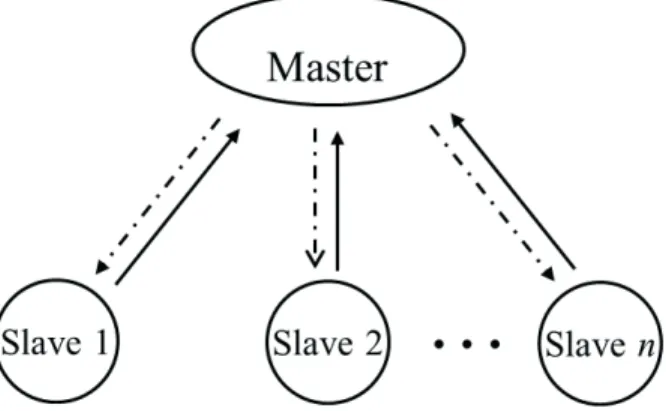
Master/Slave, an easy-to-implement structure, consists of two functions: a single Master and multiple Slaves (see Figure 1). The Master is responsible for decomposing the problem into small tasks, distributing these tasks among a farm of Slaves, as well as for gathering the partial results in order to produce the final result of the computation. The Slaves execute in a very simple cycle: get a message with the task from the Master, process the task, and send the result to the Master. Usually, the communication takes place only between Master and Slaves, which is a property desired in our problem because we assume the independence between alternatives.
Master/Slave structure may either use static load-balancing or dynamic load-balancing. In the first case, the distribution of tasks is pre-specified at the beginning of computing, which allows the Master to
participate in the computation after each Slave has been allocated a fraction of the work. The allocation of tasks can be done once or in a cyclic way. The other way is to use a dynamically load-balanced system, which can be more suitable when the number of tasks exceeds the number available processors or when the execution times are not predictable, or when the problem itself is unbalanced. In this paper, we use the dynamic load-balancing in our procedure. An important feature of dynamic load-balancing is the ability of the application to adapt itself to changing conditions of the cloud platform, not only the load of each processor, but also a possible reconfiguration of available resources. Due to this characteristic, this paradigm can respond quite well to the failure of some Slaves, which simplifies the creation of robust applications that are capable of processing the entire work with the loss of some Slaves. Readers are referred to Silvay and Buyya (1999) for more detailed discussion on Master/Slave structure, as well as some other structures.
3 FRAMEWORK CONSTRUCTION
With the properties of cloud computing and Master/Slave, we can easily construct at least two simply doable procedures. In the first procedure, Master assigns one system to one Slave or multiple systems to one Slave or one system to serval Slaves, depending on the numbers of both available Slaves and systems. In our problem, Slaves will request their own sublist containing the task specified by Master, generate samples and transfer them to Master; Master is in charge of comparison work between systems, making a decision to eliminate systems and also creating a new list. Then the idle Slaves will randomly switch to handle a nonempty sublist. In the second procedure, Master always creates a common list consisting of all survival systems and Slaves simulate all systems contained in the common list. On each Slave, whose behavior is similar to a single processor, one could apply different sampling rules to allocate the samples, e.g., the KN procedure Kim and Nelson (2006b), or the known-variance and unknown-variance procedures in Hong (2006), or simply iterating all survival systems. However, the extra cost of switching will occur when using this allocation scheme. Hong and Nelson (2005) observed this phenomena and discussed the tradeoff between sampling and switching and then attempted to minimize the total computational cost. If the switching cost is not significant, this scheme could work well. However, to avoid this unnecessary cost, hereafter we focus on the first scheme, as shown in Figure 1 and 2, where Slaves submit their results ceaselessly to Master and Master sends back the updated information, i.e., the list of survival systems, every once in a while.
Figure 1: The general Master/Slave structure. Slaves request tasks from Master and send outputs back to Master. There is no communication between Slaves.
3.1 Construction of Brownian Motion
In this subsection, we reconstruct the corresponding Brownian motions with drifts, as in Hong (2006) and design a doable, but possibly not optimal algorithm.
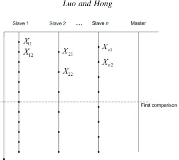
Figure 2: Generating independent samples from each Slave. Master is in charge of comparison, elimination and reallocation.
In practice, we do not care about the exact number of Slaves. The number can be greater or smaller than the number of systems, and can even change during the process because of traffic jam in the network
or failure of some nodes. For notational simplicity, we suppose there arekSlaves handlingksystems in the
beginning, e.g., Slaveisimulates samples from systemi, which follows normal distribution with mean µi
and varianceσi2,i=1, . . . ,k. If the number of Slaves exceeds the number of systems, we can simply allow
two or more Slaves to generate independent samples for one single system. If the number of Slaves is less than that of the systems, we can allocate several systems to one Slave at first. As the elimination procedure continues, the number of systems will decrease gradually, and eventually we will enter in the previous case where the released Slaves help the remaining systems. We assume that the difference between means
of the best and second best systems is greater than or equal to δ and the varianceσi2 may or may not be
equal or known for all i=1,2, . . . ,k. We aim to design an algorithm to select the best system which is
guaranteed to have the largest mean among thek systems with a probability at least 1−α. LetXi`denote
the`th sample from systemiand we require thatXi` are mutually independent, which implies that we do
not use common random numbers. The sample mean of systemiis thenXi(n) =∑n`=1Xi`/n. Lettdenote
the time point andni(t)denote the sample size of system iat timet. It is highly possible thatni(t)6=nj(t)
fori6=jdue to the asynchronous property. Generally, we want to compare the means of two systems, say
iand j, under the conditions of both unequal sample sizes and unequal variances.
Let{B∆(t),t≥0}be a Brownian motion process with a constant drift ∆, having the distribution of
B∆(t) =B(t) +∆t, t≥0,
whereB(t)is a standard Brownian motion process, see Karlin and Taylor (1975) for a rigorous definition
of Brownian motion process with drift. Let
Z(m,n) = " σi2 m + σ2j n #−1 Xi(m)−Xj(n). (1)
Hong (2006) provided a general framework of approaching Z(m,n) by B∆(t), which is stated in the
following lemma.
Lemma 1 For any sequence of pairs(m,n)of positive integers that is non-decreasing in each coordinate,
the random sequencesZ(m,n)andBµi−µj([σ
2
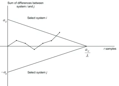
Using this result, we can determine a triangular continuation region to design IZ selection procedures
when variancesσi2 are either known or unknown (see Figure 3).
Figure 3: Triangular continuation region. Selection of system ior jas best depends on whether the sum
of differences exits the region from the top or bottom.
3.2 The Procedure
We first introduce the procedure for the known-variances case. Even though this is usually an unrealistic case, we consider it because it can help us illustrate the key idea in an easier way. The case of unknown-variances will be discussed immediately after that. The procedure is designed as follows,
Setup: Select confidence level 1/k<1−α<1, IZ parameterδ >0. Letλ such that 0<λ <δ (λ=δ/2 is used in our procedure) and
a=−1 δ ln h 2−2(1−α)1/(k−1) i . (2)
Note thatλ andadefine the triangular continuation region (see Figure 3, where ai j=a).
Initialization: LetI=∪N
i=1Ii={1,2, . . . ,N}be the set of systems still in contention, whereIi={i}be the
sublist containing systemi. Master assigns listIi to Slavei.
Screening: Slaveistarts to take samples for the given system in list Ii and submits the sample Xi` once
the`th sample is obtained,`=1,2, . . ., as well as update number of samplesni=`to the Master. Master calculates τi j(t) = " σi2 ni(t)+ σ2j nj(t) #−1 (3) and
Zi j(τi j(t)) =τi j(t)[Xi(ni(t))−Xj(nj(t))]. (4)
Systemiwill be eliminated if
for some j∈I\ {i}, whereA\B={x:x∈Aandx∈/B}. Update listI. If sublistIi is empty, randomly let Ii=Ij for some nonempty subsetIj.
Stopping Rule: If|I|=1, then stop and select the system whose index is in I as the best. Otherwise, go toScreening.
Remarks:
I. In theInitializationstep, the sublistIi may have several elements in the beginning in the case that
we have more systems than the available Slaves.
II. In theScreeningstep, ifIiis empty, an improved way is to assign the listIj who contains the system
temporarily with largest sample mean toIi. This rule will lower the frequency of reassigning the
empty list in the future.
III. In theScreeningstep, in order to reduce the communication time between Slaves and Master, we
can require the Slaves to submit batch samples instead of single sample once a time. Because the samples are generated in parallel, it is no longer efficient if we compare with all other systems when one sample is obtained, which definitely makes Master overloaded. Therefore, we may specify the frequency to require Master to do comparison and elimination. Note that the frequency depends on the problem itself.
In most cases the variances of the systems are not known in advance. One way to solve this problem is to modify the former procedure by using two or more stages, with the first stage estimating the variances. If the procedures in the subsequent stages depend only on the first-stage sample variances, Stein (1945) showed that the overall sample means are independent of the first-stage variances. Providing this property, we develop an algorithm for the unknown-variances case.
Setup: Select confidence level 1/k<1−α <1, IZ parameter δ >0, and the first-stage sample size
n0=d5 log2(k)e, where dxe=min{m:m≥x andmis an integer}. Let λ=δ/2 and abe the solution to
the equation E 1 2exp − aδ n0−1 Ψ =1−(1−α)1/(k−1), (6)
whereΨis a random variable whose density function is
fΨ(x) =2[1−Fχn2 0−1
(x)]fχ2
n0−1(x), (7)
and Fχ2
n0−1 and fχn20−1 are the distribution function and density function of a χ
2 distribution with n
0−1 degrees of freedom.
Initialization: Take n0 samplesXi`, `=1, . . . ,n0, from each system i=1,2, . . . ,k. For alli=1,2, . . . ,k, calculate S2i = 1 n0−1 n0
∑
`=1 (Xi`−Xi(n0))2, (8)the first-stage sample variance of system i. Let I =∪k
i=1Ii ={1,2, . . . ,k} be the set of systems still in
contention, where Ii=ibe the sublist containing systemi. Master assigns each Slave ithe list Ii.
Screening: Slave istarts to take samples for the given system in list iand submits the sample Xi` once
the`th sample is obtained,`=1,2, . . ., as well as update number of samplesni=`to the Master. Master calculates τi j(t) = " Si2 ni(t)+ S2j nj(t) #−1 (9)
and
Yi j(τi j(t)) =τi j(t)[Xi(ni(t))−Xj(nj(t))]. (10)
Systemiwill be eliminated if
Yi j(τi j(t))<min{0,−a+λ τi j(t)} (11)
for some j∈I\ {i}. Update listI. If sublistIi is empty, randomly letIi=Ij for some nonempty subset Ij.
Stopping Rule: If|I|=1, then stop and select the system whose index is in I as the best. Otherwise, go toScreening.
Now we state the key theorem in this paper without proofs. One can refer to Hong (2006) for the statistical validity. Without loss of generality, suppose that the true means of the systems are indexed so thatµk≥µk−1≥. . .≥µ1 andµk−µk−1≥δ.
Theorem 1 Suppose thatXi`,`=1,2, . . ., are i.i.d. normally distributed and thatXipandXjqare independent
fori6= jand any positive integers pandq. Then the unknown-variances procedure selects systemk with
probability at least 1−α.
4 AN ILLUSTRATIVE EXAMPLE
In a classic(s,S)inventory problem (Koenig and Law 1985), the level of inventory of some discrete unit
is periodically reviewed. If the inventory position (units in inventory plus units on order minus units
backordered) at a review is belows units, then an order is placed to bring the inventory position up to S
units; otherwise, no order is placed. The setup cost for placing an order is 32 and ordering cost, holding cost and backordering cost are 3, 1 and 5 per unit, respectively. Demand per period is Poisson with mean
25. The goal is to selects andS such that the steady-state expected inventory cost per review period is
minimized. Therefore, we need to define the best system as minimum expected value instead of maximum
expected value. The constraints ons andSareS−s≥0, 20≤s≤80, 40≤S≤100, and s,S are positive
integers. The number of feasible solutions is 2901. The optimal inventory policy is(20,53)with expected
cost/period of 111.1265. To reduce the initial-condition bias, the average cost per period in each replication is computed after the first 100 review periods and averaged over the subsequent 30 periods.
Because the set of feasible solutions is relatively large, this inventory problem is usually considered as an OvS problem, see Hong and Nelson (2006) and Pichitlamken, Nelson, and Hong (2006) for various optimization-via-simulation algorithms. Under the cloud framework, we can simulate all 2901 systems and select the best one in around one hour on the local small cluster.
4.1 Implementation of the Master/Slave Structure on a Small Cluster
We construct a small scaled cluster of 7 computers with 14 processors and test our algorithm with Master/Slave structure on this cluster. Each computer is installed with Ubuntu 10.04 system, a Linux-based operating system. In addition, we install Openssh package to function the remote control and the necessary Java package to run the experiments. While the local cluster is relatively small, the basic principle and functionality are essentially the same as launching a large scale of instances equipped the same operating system and softwares in Amazon EC2.
Although one can launch as many Slaves as he desires, we suggest to launch one or two Slaves for one processor according to configurations of the computers. In our setting, we have one Master and 14 Slaves on the local cluster, which is far away from the number of systems. We consider each feasible
solution(s,S)as a system and label them with 1,2, . . . ,2091. Then, we simply partition 2901 systems into
14 groups, with the first 13 groups having 210 members and the last one having 171 members, and assign each group to one Slave at the beginning.
4.2 Numerical Results
Apparently,I={1,2, . . . ,2901}=∪14
i=1Ii, whereIi={1+210(i−1),2+210(i−1), . . . ,210+210(i−1)} fori=1,2, . . . ,13 andI14={2731,2731, . . . ,2901}. We set the probability significance levelα=0.05, IZ
parameter δ =0.01 and the first stage sample sizen0=d5 log2(2901)e=58. Since we consider the best
as the minimum expected value, the elimination criterion in Eq. (11) will be modified to
Yi j(τi j(t))>max{0,a−λ τi j(t)} (12)
for some j∈I\ {i}, then Systemiwill be eliminated.
We run the algorithm for 100 replications and find that the best system (s∗,S∗) = (20,53) is always
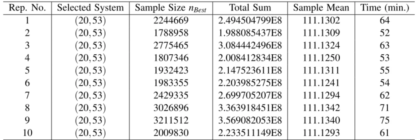
selected with various total sample sizes. Here we report the results for the first 10 replications in Table 1. Table 1: The First 10 Replications.
Rep. No. Selected System Sample SizenBest Total Sum Sample Mean Time (min.)
1 (20,53) 2244669 2.494504799E8 111.1302 64 2 (20,53) 1788958 1.988085437E8 111.1309 52 3 (20,53) 2775465 3.084442496E8 111.1324 63 4 (20,53) 1807346 2.008412834E8 111.1250 53 5 (20,53) 1932423 2.147523611E8 111.1311 55 6 (20,53) 1983355 2.203985275E8 111.1241 54 7 (20,53) 2429335 2.699705207E8 111.1294 62 8 (20,53) 3026896 3.363918451E8 111.1342 71 9 (20,53) 3211512 3.569082053E8 111.1340 75 10 (20,53) 2009830 2.233511149E8 111.1293 61
From Table 1, we find that our procedure works well on the small cluster, since it selected the best system 100 times in 100 replications. The samples sizes, as well as simulation times, are quite different, but the sample means are all close to the true mean 111.1265. By monitoring our algorithm, we note that it takes a relatively long time to eliminate one of the last two systems using the algorithm, which encourages us in the future to determine a more efficient sample rule when only several systems are left.
5 CONCLUSIONS AND FUTURE STUDY
In this paper, we develop a simple algorithm for IZ approach and use this approach to solve the classic inventory problem completely. Note that currently our numerical experiments are conducted on our small cluster. In the following step, we will implement our algorithm on Amazon EC2 cloud platform. We believe our study on the implementation of cloud computing will impact the development of computer-based simulation of R&S procedures and optimization via simulation problems.
There are some potential research directions. First, the Master/Slave structure can achieve high computational speedups and scalability. However, the centralized control of the Master could be a bottleneck when there are a large number of Slaves. Thus, it is possible to enhance the scalability of this structure by extending the single Master to multiple Masters, each of them controlling a different group of Slaves. Moreover, we can test other structures, such as the existing MapReduce structure. Second, when the computational budget is no longer a limitation, the sample size can be as large as possible, then it is reasonable and attractive to use all the information of the sample variance rather than only taking the
first-stage sample variance. To study the asymptotic validity as the number of systemskgoes to infinity is
also appealing and challenging. Third, there are another type of procedures developed from a Bayesian point of view which we do not consider in this paper, however, we believe it is worth restudying these problems since the computational budget is no longer the critical concern or limitation in designing algorithms on the cloud.
ACKNOWLEDGMENTS
This research is partially supported by the Hong Kong Research Grants Council under grants GRF 613410 and N HKUST 626/10.
REFERENCES
Apache 2011, 05. Accessed Oct. 16, 2011.,http://hadoop.apache.org/mapreduce/.
Andy Bechtolsheim 2008, December. “Cloud Computing”. Accessed Oct. 16, 2011., http://netseminar.
stanford.edu/seminars/Cloud.pdf. Seminar Material.
Buzacott, J. A., and J. G. Shanthikumar. 1993.Stochastic Models of Manufacturing Systems. Prentice Hall.
Chang, F., J. Dean, S. Ghemawat, W. C. Hsieh, D. A. Wallach, M. Burrows, T. Chandra, A. Fikes, and R. E.
Gruber. 2006. “Bigtable: a distributed storage system for structured data”. InOSDI’06: Proceedings of
the 7th Symposium on Operating System Design and Implementation, Volume 7, 205–218: USENIX Association.
Dean, J., and S. Ghemawat. 2004. “MapReduce: simplified data processing on large clusters”. InOSDI’04:
Proceedings of 6th Symposium on Operating System Design and Implementation, 137–150: USENIX Association.
Ghemawat, S., H. Gobioff, and S.-T. Leung. 2003. “The Google file system”. InSOSP’03 Proceedings of
the 19th ACM Symposium on Operating Systems Principles, Volume 37, 29–43: ACM.
Hong, J. L., and B. L. Nelson. 2005. “The tradeoff between sampling and switching : new sequential
procedures for indifference-zone selection”.IIE Transactions 37:623–634.
Hong, L. J. 2006. “Fully sequential indifference-zone selection procedures with variance-dependent
sam-pling”.Naval Research Logistics53:464–476.
Hong, L. J., and B. L. Nelson. 2006. “Discrete optimization via simulation using COMPASS”.Operations
Research54:115–129.
Karlin, S., and H. Taylor. 1975.A First Course in Stochastic Processes, Second Edition. Elsevier.
Kim, S.-H., and B. L. Nelson. 2001. “A fully sequential procedure for indifference-zone selection in
simulation”. ACM Transactions on Modeling and Computer Simulation11:251–273.
Kim, S.-H., and B. L. Nelson. 2006a.Elsevier Handbooks in Operations Research and Management Science:
Simulation, Chapter 17. Selecting the best system, 501–534. Elsevier.
Kim, S.-H., and B. L. Nelson. 2006b. “On the asymptotic validity of fully sequential selection procedures
for steay-state simulation”.Operations Research54:475–488.
Koenig, L. W., and A. M. Law. 1985. “A procedure for selecting a subset of sizemcontaining the l best
ofk independent normal populations, with applications to simulation”.Communications in Statistics:
Simulation and Computation 14:719–734.
MathWorks 2008. “Parallel Computing with MATLAB on Amazon Elastic Compute Cloud (EC2)”. Accessed
Oct. 16, 2011.,http://www.mathworks.com/programs/techkits/ec2 paper.html.
Mell, P., and T. Grance. 2009. “The NIST definition of could computing”.National Institute of Standards
Technology 53:50.
Nelson, B. L., J. Swann, D. Goldsman, and W. Song. 2001. “Simple procedures for selecting the best
simulated system when the number of alternatives is large”. Operations Research49:950–963.
Pichitlamken, J., B. L. Nelson, and L. J. Hong. 2006. “A Sequential Procedure for Neighborhood
Selection-of-the-best in Optimization via Simulation”.European Journal of Operational Research173:283–298.
Silvay, L. M. E., and R. Buyya. 1999.High Performance Cluster Computing: Programming and Applications,
Chapter Parallel programming models and paradigms, 4–27. Prentice Hall.
Stein, C. 1945. “A two-sample test for a linear hypothesis whose power is independent of the variance”. The Annals of Mathematical Statistics16:243–258.
Sun 2009, June. “Introduction to cloud computing architecture, 1st Edition”. Technical report, Sun Mi-crosystems, Inc. White Paper.
AUTHOR BIOGRAPHIES
L. JEFF HONG is a professor in the Department of Industrial Engineering and Logistics Management at the Hong Kong University of Science and Technology (HKUST). His research interests include Monte Carlo method, financial engineering and risk management, and stochastic optimization. He is currently an
associate editor for Operations Research, Naval Research LogisticsandACM Transactions on Modeling
and Computer Simulation. His email address is [email protected].
JUN LUO is a Ph.D. student in the Department of Industrial Engineering and Logistics Management at