PURDUE UNIVERSITY GRADUATE SCHOOL Thesis/Dissertation Acceptance
This is to certify that the thesis/dissertation prepared By Parisa Ghane
Entitled
SILENT SPEECH RECOGNITION IN EEG-BASED BRAIN COMPUTER INTERFACE
For the degree of Master of Science in Electrical and Computer Engineering Is approved by the final examining committee:
Lingxi Li Chair
Andres Tovar Lauren Christopher
To the best of my knowledge and as understood by the student in the Thesis/Dissertation Agreement, Publication Delay, and Certification Disclaimer (Graduate School Form 32), this thesis/dissertation adheres to the provisions of Purdue University’s “Policy of Integrity in Research” and the use of copyright material.
Approved by Major Professor(s): Lingxi Li
Approved by: Brian King 12/2/2015
BRAIN COMPUTER INTERFACE
A Thesis
Submitted to the Faculty of
Purdue University by
Parisa Ghane
In Partial Fulfillment of the Requirements for the Degree
of
Master of Science in Electrical and Computer Engineering
December 2015 Purdue University Indianapolis, Indiana
To my parents whose words of encouragement and push for tenacity ring in my ears and my siblings who have never left my side.
ACKNOWLEDGMENTS
First and foremost, I would like to express my deepest appreciation to my advi-sor, professor Lingxi Li, and co-adviadvi-sor, professor Andres Tovar, for their guidance, encouragement, support, and most of all patience throughout this work. Thank you for providing machines, tools, and study spots to make this research an appealing experience for me. I am also grateful to professor Lauren Christopher for accepting being my Committee member and giving me guidance to do better in this work.
In addition, I wish to thank many faculty and staff members at IUPUI for their helps during my master studies and contributions to my thesis work. Special thanks to professor Brian King for all supports, advices, discussions, inspirations, initiations, motivations, encouragements, and many more that I can not express in words. I would also like to thank Mrs. Sherrie Tucker for her friendly instructions and guides in the department of electrical and computer engineering. In addition, I would like to acknowledge assistance of professor Paul Salama for helping me understanding some new concepts.
Last but not least, I would like to take this opportunity to thank all the people who provided resources, and datasets to make this work easier for me. Thank you all IUPUI library staff and in particular engineering and technology librarian, Mrs. May Jafari, for spending years to collect this strong and rich library database, which has given me access to a wide range of books, journals, and papers throughout this research. Furthermore, I would like to thank Dr. Luis Carlos Sarmiento Vela for conducting the electroencephalographic experiments at the National University of Colombia and letting me use his raw datasets.
TABLE OF CONTENTS
Page
LIST OF TABLES . . . vii
LIST OF FIGURES . . . viii
ABSTRACT . . . xi
1 INTRODUCTION . . . 1
1.1 History and background . . . 1
1.2 Related works . . . 2 1.3 Applications . . . 4 1.4 Problem . . . 6 1.5 Goal . . . 9 1.6 Contributions . . . 9 1.7 Thesis outline . . . 10
2 BRAIN FUNCTIONALITY, EEG, AND BCI . . . 11
2.1 Brain and neurons . . . 11
2.2 Brain waves . . . 13
2.2.1 Delta waves (0.5 to 4 Hz) . . . 14
2.2.2 Theta waves(4 to 8 Hz). . . 14
2.2.3 Alpha waves (8 to 12 Hz) . . . 14
2.2.4 Beta waves (12 to 35 Hz) . . . 15
2.2.5 Gamma waves (35 Hz and up) . . . 15
2.3 BCI classes . . . 16
2.3.1 Invasive BCI systems . . . 17
2.3.2 Partially invasive BCI systems . . . 17
2.3.3 Non-invasive BCI systems . . . 17
Page
3 BCI STRUCTURE . . . 22
3.1 Signal acquisition . . . 22
3.2 Signal preprocessing . . . 25
3.3 Feature extraction . . . 26
3.3.1 Fast Fourier Transform (FFT) & Power Spectral Density (PSD) 27 3.3.2 Wavelet Transform (WT) . . . 28
3.3.3 Eigenvectors . . . 29
3.3.4 Autoregressive Method (AR). . . 31
3.4 Features classification . . . 34
3.4.1 Linear Discriminant Analysis (LDA) . . . 35
3.4.2 Support Vector Machine (SVM) . . . 38
4 METHODOLOGY AND EXPERIMENTS . . . 43
4.1 EEG signal recording . . . 43
4.2 Signal pre-processing . . . 45
4.2.1 Neural and non-neural components of EEG data . . . 45
4.3 Feature extraction . . . 47 4.4 Classification . . . 47 5 RESULTS . . . 51 5.1 Data pre-processing . . . 51 5.1.1 EEG segmentation . . . 51 5.1.2 Filtering . . . 53 5.2 Feature extraction . . . 55
5.3 Classifier training using known data . . . 56
5.4 Classifying an unknown data. . . 63
6 SUMMARY AND FUTURE RECOMMENDATION. . . 66
6.1 Summary . . . 66
6.2 Future recommendations . . . 68
Page APPENDICES
A DECISION TREE CONFIGURATION . . . 79
B MATLAB CODES . . . 84
B.1 Gaussian wavelet . . . 84
B.2 Preprocessing . . . 84
B.3 Dimension reduction and feature extraction . . . 86
LIST OF TABLES
Table Page
2.1 Advantages and limitations in different BCI classes. . . 19 2.2 Neuroimaging methods. . . 20 3.1 Spatial letters. . . 25 3.2 Comparison between performance of different EEG feature extraction
meth-ods. . . 32 5.1 Confusion matrix interpretation.. . . 65
Appendix Table
A.1 Confusion matrix interpretation for different methods of distance calcula-tion. . . 79
LIST OF FIGURES
Figure Page
1.1 Brain auditory and language areas. . . 7
1.2 Position of the 21 electrodes on the brains left hemisphere. . . 8
2.1 A signal propagating down an axon to the cell body and dendrites of the next cell.. . . 12
2.2 Frequency spectrum of normal EEG in a random trial from a random subject. . . 13
2.3 Normal adult brain waves. . . 15
2.4 BCI classes in different layers covering the brain [47]. . . 16
2.5 Dry electrode with pin. . . 20
2.6 Dry foam electrode fabricated by electrically conductive polymer. . . . 21
3.1 Left and right hemispheres. . . 23
3.2 10-20 standard system [34]. . . 24
3.3 10-20 system modified by American EEG society [34]. . . 25
3.4 Gaussian wavelet of order three, an example for continues wavelets. . . 29
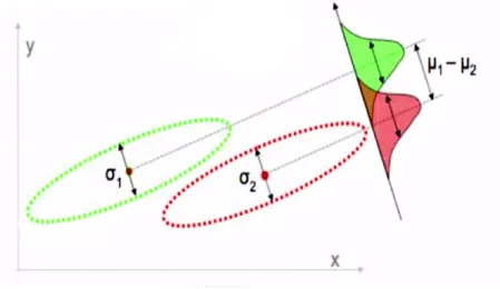
3.5 LDA versus PCA in finding a new axis for separation of red and green data. Both methods project the data on their new axis. LDA finds the red axes and PCA finds the blue one. . . 36
3.6 LDA works better than PCA in this case, because the mean of two datasets are easily distinguishable. . . 37
3.7 PCA performs better than LDA in this case, because the means of two variables are very close to each other but their variance can distinguish them. . . 37
3.8 Two classes of positives and negatives. . . 38
3.9 Widest possible street between closest elements of two groups. . . 39
3.10 Vector of deference of positive support vector and negative support vector. The dot product of this vector and a normal unit vector gives the width of the street. . . 40
Figure Page
4.1 Schematic of a common BCI. . . 43
4.2 Subject wearing the silicon EEG neuro-headset with 21 electrodes on the left hemisphere plus one frontal reference electrode. . . 44
4.3 Frequency bandwidth of components of recorded EEG. . . 45
4.4 Positives and negatives are not easily separable in this space. . . 49
4.5 Changing the space will result in easily separable datapoints. . . 49
5.1 EEG recording time frames. . . 52
5.2 Raw signals from 21 channels taken from one subject including 11 conse-qutive trials. . . 52
5.3 Raw signals for 21 channels in one trial. . . 53
5.4 Bandpass filter specifications. . . 54
5.5 Band pass filter. . . 54
5.6 Signal from one electrode before and after BPF(noise and artifact rejec-tion). . . 55
5.7 Taking average of periodograms over all datapoints gives a value for each channel. This figure shows this value for 21 channels in each class in first trial with subject one. . . 57
5.8 Taking average of periodograms over all datapoints gives a value for each channel. This figure shows this value for 21 channels in each class in first trial with subject two. . . 58
5.9 a) groups of training data, b)first iteration of applying the tree algorithm creates a new group (6), c) second iteration of applying the tree algorithm creates the group (7), d) third iteration of the tree algorithm applying on groups (7), (3), and (6) creates a new group (8), e) finally there is only two groups of (6) and (8) to classify. . . 61
5.10 Grouping classes based on their centers’ distance. . . 62
5.11 SVM training for groups of classes. . . 63
5.12 Classifying the new input dataset xk. . . 64
5.13 Confusion matrix obtained for classification. . . 65
Appendix Figure A.1 Decision tree using seuclidean distance method. . . 80
Figure Page A.2 Classification result using the tree with seuclidean distance method. . . 80 A.3 Decision tree using cosine distance method. . . 81 A.4 Classification result using the tree with seuclidean distance method. . . 81 A.5 Decision tree using spearman distance method. . . 82 A.6 Classification result using the tree with spearman distance method. . . 82 A.7 Decision tree using hamming distance method. . . 83 A.8 Classification result using the tree with hamming distance method. . . 83
ABSTRACT
Ghane, Parisa. M.S.E.C.E., Purdue University, December 2015. Silent Speech Recog-nition In EEG-based Brain Computer Interface. Major Professor: Lingxi Li.
A Brain Computer Interface (BCI) is a hardware and software system that estab-lishes direct communication between human brain and the environment. In a BCI system, brain messages pass through wires and external computers instead of the nor-mal pathway of nerves and muscles. General workflow in all BCIs is to measure brain activities, process and then convert them into an output readable for a computer.
The measurement of electrical activities in different parts of the brain is called electroencephalography (EEG). There are lots of sensor technologies with different number of electrodes to record brain activities along the scalp. Each of these elec-trodes captures a weighted sum of activities of all neurons in the area around that electrode.
In order to establish a BCI system, it is needed to set a bunch of electrodes on scalp, and a tool to send the signals to a computer for training a system that can find the important information, extract them from the raw signal, and use them to recognize the user’s intention. After all, a control signal should be generated based on the application.
This thesis describes the step by step training and testing a BCI system that can be used for a person who has lost speaking skills through an accident or surgery, but still has healthy brain tissues. The goal is to establish an algorithm, which recognizes different vowels from EEG signals. It considers a bandpass filter to remove signals’ noise and artifacts, periodogram for feature extraction, and Support Vector Machine (SVM) for classification.
1. INTRODUCTION
Communication between human brain and external world is an interesting way for paralyzed people to conduct their daily activities much easier. This excites scholars to work on a new non-muscular path to send commands from ones brain to external tools. There are lots of works on designing a faultless BCI system presented in last few decades. Although there are many big achievement in this field, it looks like applications of BCI for speechless people has not been into consideration that much. Designing a BCI system for speech recognition from EEG signals would be a big step toward the expansion of BCI applications.
1.1 History and background
Working on BCIs started from 1924 by German neurologist ,Hans Berger 1. He
started studying brain circulation, psychophysiology and brain temperature at uni-versity. He first started with inserting two silver wires under the patients scalp, at the front and back of the head. Later his research ended with invention of electroen-cephalography (EEG). He could record the first human brain electrical activity in 1924 and published his paper in 1929 [1]. After a few years, EEG got very popular among researchers in United States, England, and France [2]. Berger was also the first person to introduce different brain waves such as alpha waves, which is also called Berger’s waves. His analysis of EEG wave diagrams with brain diseases opened a new window for the research of human brain activities. Nowadays, After several decades of research and laboratory experiments on EEG, we are still far from having EEG recording and applications useful for daily tasks.
1http://www.brainvision.co.uk/blog/2014/04/the-brief-history-of-brain-computer-interfaces (last
Defense Advanced Research Projects Agency of USA initiated program to ex-plore brain communications using EEG in 1970. The term Brain Computer Interface (BCI) was made up by Professor Jacques J. Vidal (from University of California, Los Angeles) in his article in 1976 [3–5].
Several years after BCI introduction, in 1998, the first invasive measurement was done to produce high quality brain signals. In 1999, BCI helped a quadriplegic for limited hand movements. Training monkeys to control a computer cursor in 2002 was next big step in BCIs. First BCI game was release to the public in 2003, and first control of a robotic arm by a monkey brain was in 2005 [4, 6].
BCIs has had a significant growth due to the applications of use of neural electrical activities in control of machines. Understanding neural mechanism of communication between human and machine has become a research issue that has been considered more in last few decades. The measurement of brain electrical activities, Electroen-cephalography (EEG), plays an important role in non-invasive BCI systems. Depend-ing on the function of a BCI system, different electroencephalographical (EEG) signals have to be used [7, 8]. These signals include slow motor imagery potentials [9–11], P300 potentials [12, 13], and visual evoked potentials (VEP) [14, 15].
1.2 Related works
[4, 16] give general reviews of BCI systems. A review of EEG measurements is done by M. Teplan in [17]. Extracting information and features for a BCI system is the main concentration of Waldert and his colleagues in [18]. Also, McFarland with his coauthors and M. J. Safari with his colleagues provide overviews of feature extraction and translation methods [19, 20]. Furthermore, Lotte, et al. concentrate on classifications in [21].
Among successful researches done in BCI fields, we can mention Neural Signals inc. founded by Philip Kennedy in 1988. The first intracortical BCI, which tested on monkeys, was built by him and his colleagues [22]. Cats where the subjects for Yang
Dan’s team at university of California at Berkelely research. The cats were shown some pictures and their neural signals were recorded and then were used to reproduce the images in cat’s sight [23]. Other examples of successful projects in BCI is the one done by was done by Miguel Nicolelis, a professor of Duke university in North Carolina. He and his team recorded and then decoded mental activities first in rats and then in monkeys to regenerate their movements. The first result of their project was an open loop BCI for remotely control a robot. Then they expanded this system to a closed-loop BCI with feedback meaning that monkeys could see the robot moving and so that the BCI system received feedback [24]. Some other BCI developments are the ones that John Donoghue and Andrew Schwartz have done at Brown University and the University of Pittsburgh respectively. They were the first people who built BCI systems using recording of only a few neuron activities. Donoghue and his team had monkeys to follow the movement of a mark on a computer screen in one project, and control a prosthetic arm [25]. The monkeys brain were examined through the experiments by Schwartz and his research team [26].
Since 2010, there has been an annual BCI research award program hosted by one of the institutes known for BCI research. The host is responsible to judge and award an outstanding and innovative research in the field of Brain-Computer Interfaces. The list bellow includes a record of outstanding works that won the competition from 2010 to 20152.
2010 ”Motor imagery-based Brain-Computer Interface robotic rehabilitation for stroke” by Cuntai Guan, Kai Keng Ang, Karen Sui Geok Chua and Beng Ti Ang, from
Agency for Science, Technology and Research, Singapore.
2011 ”What are the neuro-physiological causes of performance variations in brain-computer interfacing?” by Moritz Grosse-Wentrup and Bernhard Schlkopf, from
Max Planck Institute for Intelligent Systems, Germany.
2012 ”Improving Efficacy of Ipsilesional Brain-Computer Interface Training in Neu-rorehabilitation of Chronic Stroke” by Surjo R. Soekadar and Niels Birbaumer, from Applied Neurotechnology Lab, University Hospital Tbingen and Institute of Medical Psychology and Behavioral Neurobiology, Eberhard Karls University, Tbingen, Germany.
2013 ”A learning-based approach to artificial sensory feedback: intracortical mi-crostimulation replaces and augments vision” by M. C. Dadarlata,b, J. E. ODohertya, P. N. Sabesa,b fromDepartment of Physiology, Center for Integra-tive Neuroscience, San Francisco, CA, US, bUC Berkeley-UCSF Bioengineering Graduate Program, University of California, San Francisco, CA, US.
2014 ”Airborne Ultrasonic Tactile Display BCI” by Katsuhiko Hamada, Hiromu Mori, Hiroyuki Shinoda, Tomasz M. Rutkowski, from The University of Tokyo, JP, Life Science Center of TARA, University of Tsukuba, JP, RIKEN Brain Science Institute, JP.
2015 The meeting will be held in Chicago, Illinois, USA by the Department of Bio-sciences and Informatics - Faculty of Science and Technology, Keio University, Japan.
1.3 Applications
Different EEG recordings are used in various areas and applications of BCIs. In the past, the main application of BCI was in medical purposes to help paralyzed people. Nowadays, However, it is being used for people with normal health conditions as well. Gaming and entertainment are examples of applications that motivate designers to make faster, cheaper, and user-friendlier systems. Other applications are in operator monitoring and lie detection [27]. One of the biggest advantages of EEG, over other brain activity measurement methods, is high speed of signal recording. However, it does not have a good spatial resolution and has to be combined with some other
methods like MRI when high spatial resolutions are required. The most common applications of measurement and study of EEG data in humans and animals are as following [17]:
• Monitor alertness, coma and brain death.
• Locate areas of damage after an accident, head injury, stroke, tumour, etc.
• Test afferent (the central nervous system) pathways.
• Monitor cognitive engagement.
• Produce biofeedback situations, alpha, etc.
• Control anaesthesia depth.
• Investigate epilepsy and locate seizure origin.
• Test epilepsy drug effects.
• Monitor human and animal brain development.
• Test drugs for convulsive effects.
• Investigate sleep disorder and physiology.
Also, most common applications of BCI systems are in the list bellow:
• Communication with external world.
• Control of robots and objects.
• Game and entertainment.
• Operator monitoring.
• Lie detection.
1.4 Problem
BCIs design and implementation have always been a hard problem. Some reasons are difficulties of signal recording and knowledge requirements from multiple fields. The signal recording is difficult since 1) EEG recording always suffer from different types of artifacts, 2) EEG is a very noisy signal (low signal to noise ratio), 3) all sensors record almost the same signals (they are mathematically hard to distinguish from each other), 4) EEG signal depends on several unknown parameters (person specific, task specific, other variables), 5) in capturing EEG signals we have to consider many factors such as non-brain signals, head motions, muscle movements, and some other unexpected stimulus, and 6) large connections of neurons are involved in many different activities. In other words, many neurons fire at the same time, so they all affect the activity measurements. Two reasons are internally generated events and stimulation of cascade of related processes by an external event, for example a flash of light triggers a bunch of changes into the brain.
Furthermore, a wide range of knowledge is required such as methods and models specific to the nature of brain, statistics, linear algebra, signal processing, pattern recognition, and machine learning. However, on the other hand, there are many other problems that are similar to BCI design like speech recognition, pattern recognition, image processing, control systems, and robotics.
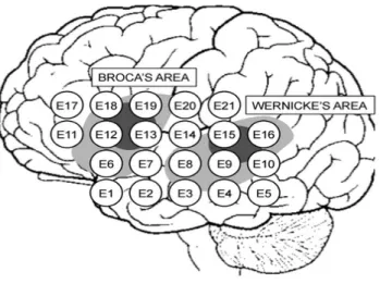
One of the problems that has been forgotten in last decades is design of a BCI system that can help speechless people to talk to the environment. This requires a system to recognize imagination of words in mind. Identification of different words needs recognition of different vowels [28]. It needs to record the brain electrical activities from the language area to have signals from speech imagination. Since different functions are assigned to various parts of brain, there is no need to measure activities all around the brain. There will be voltage changes in the posterior-superior temporal lobe, or Wernickes area, and in the posterior inferior frontal gyrus, or Brocas
area, when a person mentally pronounces a word [29] [30] (Figure 1.1)3. So that, there
should be signal recording from left hemisphere. In this project we worked with the signals coming from imagination of one of five English vowels /a/, /e/, /i/, /o/, and /u/. In some literature this process is called silent speech, in which a subject mentally speaks without generating acoustic signals [31].
Fig. 1.1: Brain auditory and language areas.
The EEG signals for this work have been collected from 20 individuals at the National University of Colombias Clinical Electrophysiology Laboratory, with the same noise and brightness levels for all individuals. Everyone on the experiment was in good health condition with their eyes closed wearing a neuroheadset with 21 electrodes plus one ground and one reference electrode. All the electrodes were places in the left hemisphere, and labeled from E1 to E21. Figure 1.24 show the position of
electrodes in the EEG data recording experiment. The ground electrode was located on the lobe of the left ear, and the reference electrode was located within the EEG
3http://mrmikesibpsychology.weebly.com/physiology-and-behaviour.html (last accessed:
12/02/2015)
4The experiment was done by Dr. Luis Carlos Sarmiento Vela and his colleagues at the Clinical
neuroheadset in the medial part of the forehead. In order to locate the neuroheadset in each subject, two reference points were used. The first point was the nasion and the second point was the left preauricular ear. To place each electrode on the scalp, the surface was first cleaned with an abrasive and later a gel conductor was applied. The lights were on and off periodically. The subjects have been asked to think about a specific vowel form /a/, /e/, /i/, /o/, and /u/ while the light is on and try to enter the relaxing state when the lights are turned off. The EEG signals were recorded by NicoletOne (Natus, San Carlos, California), amplified by Nicolet v32 amplifier, and processed using the software Nicolet VEEG (Natus, San Carlos, California). The sampling frequency was set to 500 Hz. The recorded signals are imported into Matlab in the form of two-dimensional arrays.
Fig. 1.2: Position of the 21 electrodes on the brains left hemisphere.
Nicole is specifically designed for EEG purposes by neurology team in Natus Medi-cal Incorporated Company provides a high quality diagnostic information. It can also be used to investigate LTM (Long Term Monitoring), Sleep, EP (Evoked Potential), and EMG (Electromyography). Due to NicoletOne’s high quality, ease of use, low cost, flexibility, and several available add-on packages, it is widely being used in BCI research labs.
1.5 Goal
The goal is to answer this question: is it possible to build a non-invasive brain computer interface system for vowel recognition? Reaching this goal, we can move forward to the next steps of silent speech recognition. The next step can be either identification of vowels and consonants or manipulation of the algorithm for using a portable headsets with different number of electrodes. Recognition of vowels and consonants will make the system more applicable in a wide range of speech recog-nition, like recognition of words and sentences. On the other hand, using portable EEG recording tools will give users this opportunity to use the system in their daily activities no matter in which place they actually are. This thesis focuses on the first step, which is recognition of English vowels using a non-portable EEG measurement system.
1.6 Contributions
Considering the problem and goal, we tried to implement an algorithm to take the raw signals as input and return a class label as an output. To reach this purpose, we needed to first preprocess the data and extract some of their important features, and then train a classifier, which can group all the data into 5 classes.
In order to work with the input signals easier and more accurately, we broke them into smaller pieces in such a way that no information gets lost. Then each piece was passed trough a bandpass filter to get rid of the high frequency noise and low frequency artifacts. After normalizing the filtered signals, we used periodogram to find the power spectral density as data features and meanwhile to reduce the size of the data. Sending these features to our classifier training system resulted in 4 binary classifiers based on support vector machines. Finally we used the whole system to predict that to which of 5 groups a new raw signal belongs.
It should be noted that this thesis focuses on 3 major parts: raw signals pre-processing, feature extraction, and classification (classifier training and new signals prediction). Details of each part are explained in this file. The EEG signal acquisition part of our system is done by Dr. Luis Carlos Sarmiento Vela and his colleagues at the National University of Colombia. The rest is literature review and some clarifications on methods that are common in BCI fields and the ones that we used.
1.7 Thesis outline
This thesis is divided into 5 chapters. Here is a list of chapters description:
Chapter 2 defines some of the key concepts that are being used in EEG based BCI
systems. It explains about the function of different parts of brain and how to measure these activities using the state of the art technologies. Furthermore, creation of EEG signals and different types of brain waves is described. In this chapter, different classes of a BCI system and technologies are introduced.
Chapter 3 talks about the common structure of BCI systems. It elaborates each
part of the system and some of the most used methods for each part. In this chapter, you can find the general workflow for a step by step BCI system design.
Chapter 4 shows the work flow of this thesis including experiments and algorithms.
This chapter elaborates the process of training and classifying 5 groups of data using Periodogram, Decision Tree, and Support Vector Machines.
Chapter 5 summarizes the whole project and gives some recommendations for
2. BRAIN FUNCTIONALITY, EEG, AND BCI
The measurement of electrical activities in different parts of the brain is called elec-troencephalography or EEG. There are lots of sensor technologies with different num-ber of electrodes to record brain activities along the scalp. Each of electrodes captures the weighted sum of each neurons activity from the areas in the brain around that electrode, so more electrodes give more accuracy. This chapter explains about how electrical signals are generated in brain and how electrodes can capture these signals. It also talks about common EEG and BCI technologies.
2.1 Brain and neurons
Active nerves in brain generate electrical current, which in turn produces mag-netic field and changes voltages in scalp. These can be measured and recorded as Electromyography (EMG) and Electroencephalography (EEG) respectively [32]. Electroencephalography (EEG, discovered by Hans Berger, helps us to look at brain activities without any health hazard, and even in a lower price rather than other mea-surement methods. The identification of electrographic patterns requires recognition of electrical sources and fields [33].
The brain consists of almost 100 billion nerve cells or neurons. If we consider a neuron as a switch that has on and off states, we can say that it is off while resting and on during sending electrical signal. This signal is sent through a wire called axon in which the membrane carries ions with electrical charges such as sodium (N a+),
potassium (K+), chloride (Cl−), and calcium (Ca2+). Each of axons of these billion
neurons generate a very small electrical charge, which helps the neurons to transmits information through electrical and chemical signals. Neurons can connect to each other to form neural networks.
Fig. 2.1: A signal propagating down an axon to the cell body and dendrites of the next cell.
A neuron typically has a cell body (soma), dendrites, and an axon. Dendrites arise from the cell body and travel from micrometer to meters in different species, having several branches. The cell body of a neuron often has multiple dendrites, but never more than one axon. However, an axon may branch hundreds of times before it terminates. At the majority of synapses, signals are sent from the axon of one neuron to a dendrite of another. Figure 2.1 1, explains a signal propagation of a neuron and
its transmission to the next neuron.
As explained, a neuron generates electro-chemical signals when transmitting in-formation. This neurons’ activities are measured in microvolts (µV), and frequency spectrums. The amplitude of the EEG is about 100µV when measured on the scalp, and about 1-2mV when measured on the surface of the brain. The bandwidth of this signal is from under 1Hz to about 50Hz, as demonstrated in Figure 2.2 [34]. The combination of electrical activity of the brain is commonly called a brainwave pattern, because of its cyclic wave-like nature. Brainwaves are produced by synchronized electrical pulses from masses of neurons communicating with each other. Brainwaves are divided into smaller bandwidth intervals or different brainwave types. Depending
on what a person is doing, brainwaves will change and move from one type to another. Following is different brain waves with their specifications like frequencies, amplitudes, mental states, and such that.
Fig. 2.2: Frequency spectrum of normal EEG in a random trial from a random subject.
2.2 Brain waves
Brain waves are detected using sensors placed on the scalp. They are divided into bandwidths to describe their functions (as defined bellow), and are a metric of relaxation and consciousness. For example, delta waves are slow, but gamma waves are fast, sensitive, and complex (Figure 2.3 2). Our brainwaves change according to
what we are doing and feeling. When slower brainwaves are dominant we feel tired, slow, lazy, or dreamy. The higher frequencies are dominant when we feel wired, or hyper-alert. Brainwave speed is measured in Hertz (cycles per second) and they are dived into bands of slow, moderate, and fast waves.
2http://www.zenlama.com/the-difinitive-guide-to-increasing-you-mind-power (last accessed:
2.2.1 Delta waves (0.5 to 4 Hz)
Delta waves has lowest frequency. They are the slowest but high-amplitude brain-waves. They happen in deep dreamless sleep mostly when person is unconscious. healing, regenerating and resetting of the body happens only in this state. They have also been rarely found in some continues attention tasks [35].
2.2.2 Theta waves(4 to 8 Hz)
Theta waves occur in light sleep and extreme relaxation. This state is known as a gateway to deep learning and memory. In theta, person has a very limited sense from external world but a very strong focus on a specific thing.These signals are also dominant in deep meditation. In this state, person is in a dream, or in a very special state of relaxation or intuition beyond normal conscious awareness. It is very receptive mental state that has proven useful for hypnotherapy, as well as self-hypnosis using recorded affirmations and suggestions [36, 37].
2.2.3 Alpha waves (8 to 12 Hz)
Alpha waves is the state of awake but relaxed resting and also not processing much information. They are dominant during quietly flowing thoughts, and in some meditative states. The brain is naturally in this state when an individual gets up in the morning and just before sleep. When one closes eyes, brain automatically starts producing more alpha waves. Studying EEG activities of experienced meditators reveal strong increases in alpha activity. Alpha activity has also been connected to the ability to recall memories, lessened discomfort and pain, and reductions in stress and anxiety. For more information about alpha waves see [38–42].
2.2.4 Beta waves (12 to 35 Hz)
Beta waves are present in our normal waking state of consciousness. This state is also known as wild awake. Brain goes into this state when a person is completely conscious and active. Active calm, focusing, stress, anxiety, judgement, decision making, problem solving, and all conscious activities fall into this type of waves. Some mental or emotional disorders such as depression and ADD can be caused from lack of beta activities in one’s brain. Stimulating beta activity can improve emotional stability, energy levels, attentiveness and concentration. For more information on beta waves see [43, 44].
2.2.5 Gamma waves (35 Hz and up)
Gamma waves are the fastest type of brain waves (high frequency) and relate to simultaneous processing of information from different brain areas. In this type, information are passed rapidly and happens when brain is highly active. Gamma waves have been shown to disappear during deep sleep induced by anesthesia, but return with the transition back to a wakeful state. For more information see [45, 46].
The signals and messages that are generated by BCI users’ brain pass through external wires and computers instead of the normal pathway of nerves and muscles. BCI systems make it easy to interact with the people who can not or do not like to use their muscles for any reason [4]. BCIs can be placed into two categories of dependent and independent. In order to have a dependent BCI, we need to have some knowledge about the activities that is being carried out. For example in the experiment of a screen with flashing letter, the user can choose a letter by directly looking at it. In contrast, an independent BCI is a case that does not need any of muscle activities or brains normal output pathway, like the screen with flashing letter in which the person can choose a letter not by gazing at it, but by thinking about it.
2.3 BCI classes
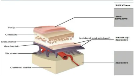
Generally, everything that is being controlled by a computer can be controlled by a BCI system. Depending on the required speed and accuracy, applications, patient states, and available equipment different types of BCI has been offered. There are basically three types of BCI systems: invasive, Partially invasive, and noninvasive. Figure 2.4 and table 2.1 3 briefly show these three types of BCIs.
Fig. 2.4: BCI classes in different layers covering the brain [47].
2.3.1 Invasive BCI systems
Invasive BCI systems are those that need to implant electrodes on or near the surface of the brain, directly into the grey matter, during neurosurgery. Signals are in the highest resolution and quality but after a while the signals become weaker, or even non-existent, as the body reacts to a foreign object in the brain. On the other hand it requires electrodes to be implanted through a surgery with health hazards One of the under research goals for invasive BCIs are to help people with sight damage and those who are seriously paralyzed [48].
2.3.2 Partially invasive BCI systems
Partially invasive BCI systems are another type of BCIs which records signals from electrodes placed inside of the skull, but outside the grey matter. An electrode grid is being implanted by a surgical process. They produce better resolution signals than non-invasive BCIs, because there is no bone tissue to deflects and deforms signals and have a lower risk of forming scar-tissue in the brain than fully invasive BCIs. Partially invasive BCI shows potential for real world application for people with motor disabilities [49, 50].
2.3.3 Non-invasive BCI systems
Non-invasive BCI systems are those which do not need any surgery to penetrate or break any part of scalp. Non-invasive systems are easy to wear without any dis-comfort. However, non-invasive implants produce poor signal resolution because the the electromagnetic field generated by neurons are dispersed and blurred while pass-ing through the skull. Although the waves can still be detected it is more difficult to determine the area of the brain that created them or the actions of individual neurons. FMRI is one of the well-known technologies that measures brain activities by detecting changes in blood volume. this method has two main advantages: no
surgery hazard and high space resolution Most non-invasive systems use electrodes placed on the scalp. Non-invasive measurements are commonly used in research and most of medical applications. In this research we consider this type of BCIs.
EMG and regular EEG are non-Invasive measurements, which means there is no need for penetrates or breaks in scalp. On the other hand, there are some brain activities recording that are known as invasive measurements. An example is Elec-trocorticography (ECoG) or intracranial EEG (iEEG) in which electrodes should be directly implanted on the cortex surface. They shows higher resolution compared to EMG and EEG but requires electrodes to be implanted through a surgery with health hazards. Medical clinics prefer to use non-invasive methods in neuroimaging. FMRI is one of the well-known technologies that measures brain activities by de-tecting changes in blood volume. this method has two main advantages: no surgery hazard and high space resolution
2.4 EEG capturing tools in non-invasive BCIs
Electrophysiological experiments consider the electrical features activities of bio-logical cells and tissues. In this field we put measurement tools in some important zones and study changes in recorded voltages. However, hemodynamic activities are those ones which are involved with the process of body adjustment while delivering glucose and oxygen to some tissues. Delivered glucose and oxygen increase activity of neurons in those body tissues. Some clinical methods like Functional Magnetic Res-onance Imaging (FMRI) can measure this change in neuronal brain activities. Table 2.2 gives a summary of neuroimaging methods [16].
The electrodes, whether invasive or non-invasive, capture neuron activities. These activities are sent to a computer, which has to use a software to translate the brain signals into computer commands. Different BCI systems use different types of EEG headsets with different types of EEG electrodes. There are basically two types of electrodes: wet and dry.
Table 2.1: Advantages and limitations in different BCI classes. BCI Class Predominant Platform Advantages Limitations Non-invasive EEG • Inexpensive. • No surgical implantation.
• Less training requirements
for using.
• Inference from non
corti-cal. stimuli
• Low quality.
Partially
Invasive ECoG
• Higher resolution than
non-invasive.
• No cortical damage.
• Good signal-to-noise ratio.
• Low clinical risk.
• Long-term stability.
• Neurosurgical
implanta-tion required.
• Not studied in
motor-impaired patients. Invasive Cortical multi-electrode array
• High performance and rate
of data output.
• Direct recording of cortical
neuron potentials.
• Vascular and neuronal
damage.
• Lack of signal stability
over time.
• Neurosurgical
Table 2.2: Neuroimaging methods.
Neuroimaging Activity Direct/Indirect Spatial Risk Portablility
method measured measurement resolution
EEG Electrical Direct ∼10 mm Non-invasive Portable
MEG Magnetic Direct ∼5 mm Non-invasive Non-Portable
ECoG Electrical Direct ∼1 mm Invasive Portable
fMRI Metabolic Indirect ∼1 mm Non-invasive Portable
BCI has been started with wet electrodes, and conductive gel. Preparation of wet electrodes are more difficult than the dry ones, which is an obstacle to use EEG-BCI system day to day for patients with impaired mobility. Scrubbing of the scalp sig-nificantly increase the signal resolutions, but it would be an unpleasant experience for almost all subjects. Also, having wet electrodes on the skin for several frequent sessions heighten skin-sensitivity. Besides, over hours of use, it requires regular main-tenance as the conductive gel dries and degrades signal quality. So that there has been several efforts to develop dry electrodes. However, studies show that additional work is needed before dry electrodes become an alternative to standard wet electrodes for the recording of EEG signals in clinical and other applications with long-term ex-posures [51].
Fig. 2.6: Dry foam electrode fabricated by electrically conductive polymer.
Nowadays new dry EEG electrodes progresses give rise to a wide range of appli-cations other than clinical appliappli-cations. Some advantages of dry electrodes, such as gel-free operation, make them easy to frequently use. Robust dry EEG electrodes are one of the key issues to practically develop BCI technologies. Dry electrodes are sub-ject to several challenges since they do not use the electrolytic gel to penetrate hair and contact the skin. They have to be designed in a way to directly touch the scalp. Also, the location of the electrode should be accurate to reduce artifact and noises as much as possible. Figures 2.5 4 and 2.6 5 show two types of common dry electrodes. The electrodes can be installed on a headset or helmet. They can be whether with a conductive gel, or dry electrodes which does not use the gel. There are two major types of tools that are being used to capture EEG signals in non-invasive BCIs: EEG caps with wet electrodes and EEG headsets with dry electrodes [17].
4http://www.gtec.at/Products/Electrodes-and-Sensors/g.Electrodes-Specs-Features (last accessed:
12/02/2015)
3. BCI STRUCTURE
BCI systems can be used in a wide variety of applications such as communication and control, operator monitoring, lie detection, gaming and entertainment, health, and help to paralyzed people. However, before reaching any of these goals several steps have to be passed. Similar to any other systems, a BCI has inputs, outputs, several components in between to translate input to outputs, and in some BCIs a feedback circuit to make the system stable all the time. More precisely, first step to design a BCI system is to provide a biocompatible EEG signals recording system, second is to develop an algorithm which can decode the messages in the EEG data with a good accuracy, and last is to create commands to send to the target system, which can be a computer, or a moving object, or a emotion detection system, or such that [4].
3.1 Signal acquisition
BCI systems use information from brain activities to identify the user’s intention. As shown in figure 3.1 1, different functions are assigned to various parts of brain, so
depending on the activity and intention, different groups of neurons will be activated. The brain is a very busy organ and is the control center for body. It runs all organs such as heart and lungs. All of senses, sight, smell, hearing, touch, and taste depend on brain functionality. For example, tasting food with the sensors on tongue is only possible if the signals from taste buds are sent to the brain. Once in the brain the signals are decoded. The sweet flavor of an orange is only sweet if the brain tells so. This highlights the role of recording brain activities as well as converting them to electrical signals.
Fig. 3.1: Left and right hemispheres.
EEG recording systems measure difference of potentials between two electrodes, which have been placed on an active neuron, and another neuron in resting state. As explained before, EEG signals depend on several unknown parameters (person specific, task specific, other variables) and always suffer from different types of arti-facts. The reason of this variability can be some biological or experimental facts like: 1) relevant functional map differs across individuals, 2) sensor locations differ across recording sessions, 3) brain dynamics are not the same at all time scales (each week something will be change in ones brain), and so on.
In order to deal with some of EEG measurement variabilities, standard systems are being used to locate sensors on scalp. These methods are developed to ensure standardized reproducibility so that a subject’s studies could be compared over time and subjects could be compared to each other. One of popular international methods is ten-twenty system, which is based on proportional measurements between easily identified skull landmarks and provides adequate coverage of all parts of the head. Figure 3.2 shows internationally standardized ten-twenty system electrode setup.
According to the ten-twenty system there are 21 electrodes placed on the scalp, as shown in Figure 3.2. To locate these electrodes the following steps has been considered: there are two reference points which are called Nasion and Inion. Nasion is the delve at the top of the nose, level with the eyes; and Inion is the bony lump at the base of the skull on the midline at the back of the head. From these points, the skull
Fig. 3.2: 10-20 standard system [34].
perimeters are measured in the transverse and median planes. Electrode locations are determined by dividing these perimeters into 10% and 20% intervals. Ten-twenty system has been widely used in the EEG cap designs since it was introduced.
The international ten-twenty system of electrode placement, originally proposed in 1958 [52]. It is widely being used as a recommended standard method for recording scalp EEG. Recently, the American EEG Society has made some modifications to the original alphanumeric. According to this new modified system, the original T3, T4, T5 and T6 are now referred to as T7, T8, P7 and P8 respectively. This modifica-tion allows standardized extension of electrode placement in the sub-temporal region (e.g., F9, T9, P9, F10, T10, P10) and designates named electrode positions in the intermediate coronal lines between the standard coronal lines (e.g., AF7, AF3, FT9, FT7, FC5, FC3, FC1, TP9, TP7, CP5, CP3, CP1, PO7, PO3 and so on)(Figure 3.3). Letters specifying the spatial locations are in table 3.12.
Fig. 3.3: 10-20 system modified by American EEG society [34].
Table 3.1: Spatial letters.
Letter Location C Central P Parietal F Frontal T Temporal O Occipital 3.2 Signal preprocessing
Once the EEG signal is captured, we are good to move toward processing, pattern recognition, classifier training, and classification of the data. In every EEG recording experiments, possible non-neural signals, such as noises and artifacts, are inevitably added up with the actual brain signals. Removing these non-neural part of the data is the first step to make signals ready for later analysis. In EEG signal processing, first, we need to use filter to remove some unwanted components of the signal. Filtering
is a method of signal processing, which deletes some frequencies and pass the rest to remove some background noises and artifacts of the signal. There are several types of filters for EEG signals processing. Some common filters used in EEG signal processing are:
• Constant filters, which have constant dynamic for all sampling times.
• Spatial filters like Independent Component Analysis (ICA) [53, 54].
• Temporal filters like moving average filters [55, 56].
• Frequency selective filters like high pass, low pass, band pass, band stop filter [28, 57].
As explained before, EEG signals are in the frequency domain below 60Hz. A high pass filter can remove any components of the signal which are in frequency higher than 60Hz. These components mostly come from background noise [58].
3.3 Feature extraction
Classification of patterns based on sampled waveforms results in poor performance. Hence, extraction of characteristic features from the data can increase the classifica-tion performance. Recorded EEG signals consist of a large number of simultaneous fired neurons. In order to select a suitable classifier, it is required to find any or all of the the sources, properties, and features of the data. Four most common groups of features are time-domain features (TDF), frequency-domain features (FDF), wavelet features (WF), and cepstral features (CF) [59].
The recorded EEG data can be quantified as voltage versus time, in the time-domain analysis, and as power versus frequency, in frequency time-domain analysis. Both forms of analysis can be used for EEG-based communication [60]. In time-domain, changes in the form or magnitude of voltage can function as a command. They are referred to as an evoked potential or evoked response. For example, in flashing letters
experiments, the evoked potentials shows that if the person wants to pick that letter or not. [60, 61] In the frequency-domain, the commands are the changes in amplitude of the signal in a specific frequency band. They are referred to as a rhythm. The major works done on cursor control on a computer screen is an example of EEG processing in frequency domain [62–64]. Bellow is a discussion of different common methods of interest. Table 3.2 from [65] compares the performance of these feature extraction methods and their general advantages and disadvantages.
3.3.1 Fast Fourier Transform (FFT) & Power Spectral Density (PSD)
Fast Fourier Transform (FFT) in signal processing is the most widespread method that analyzes data using mathematical tool. Generally, Fourier transform finds the spectrum of any type of signals using the equation 3.1. However, it is not being used for non-deterministic variables. Instead people use Power Spectral Density (PSD) for stochastic processes, in which the distribution of signal’s power is studied over different frequencies. PSD can be interpreted as the Fourier transform of the auto-correlation function and is calculated as equation 3.2.
X(ω) =
Z +∞
−∞
x(t)e−jωtdt (3.1) where x(t) is a deterministic signal in time domain and X(ω) is the represents the Fourier transform of the signalx(t).
Sxx(ω) =
Z +∞
−∞
Rxx(τ)e−jωτdτ (3.2)
where Rxx(.) is autocorrelation function and Sxx(ω) shows PSD.
There are many features to extract from data for machine learning purposes and specifically, in the field of signal processing, power spectral density is widely used as a feature of the signals of under study because it is both easily measurable and observable [66, 67]. It shows that how much power in each frequency a signal has and in this way describes the specific features from different data.
3.3.2 Wavelet Transform (WT)
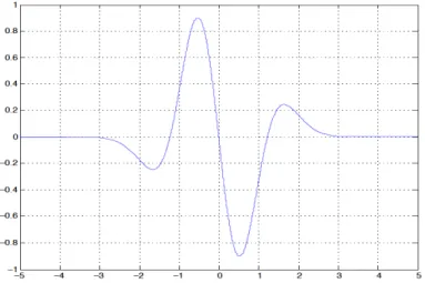
In Wavelet Transform (WT) the process includes finding a set of basis function and decompose the signals onto them. These basis functions are called wavelets. The prototype wavelets are called mother wavelets. The basic functions are made up from extended, contracted, and/or shifted versions of mother wavelets [68]. As an example of a basic function, figure 3.4 shows a Gaussian wavelet of order three. Equation 3.3 shows the general wavelet transform formula, which also represents the Continues Wavelet Transform (CWT) [69].
Xw(a, b) =
Z +∞
−∞
x(t)ψa,b∗ (t)dt (3.3) wherex(t) is the unprocessed signal, which can be EEG signals, a stands for dilation (scaling parameter), and b represents translation parameter. ∗ is the complex conju-gate symbol, functionψa,b(t) is calculated from ψ(t), and ψ(t) is the wavelet that we
has been chosen as the mother wavelet.
ψa,b(t) = 1 p |a|ψ t−b a (3.4) The wavelet transform or wavelet analysis can be regarded as a successful solution for shortcomings of the Fourier transform. In fact Fourier transform is a special case of wavelet transform whereψ∗a,b=e−jωt. The main difference is that Fourier transform decomposes the signal into sines and cosines, but the wavelet transform uses functions that are localized in both the real and Fourier space [69].
Wavelet transform is widely being used to reduce the signals parameters without much changes in the original signal [70]. It has also been applied on the EEG data as a spectral estimation strategy for the feature extraction purpose. The main focus in wavelet problems is to re-express any function as an infinite series of wavelets [71–73]. Wavelet transforms can be continuous wavelet transform (CWT) or Discrete Wavelet Transforms (DWT) [74, 75]. The DWT is a modified version of CWT when it can only be scaled and translated in discrete steps.
Fig. 3.4: Gaussian wavelet of order three, an example for continues wavelets.
3.3.3 Eigenvectors
This method is used to find frequency and power of a signal which is artifact dom-inated measured. There are a few eigenvector methods such as Principal Component Analysis (PCA), MUSIC, and Pisarenkos method [76–78]. Eigenvector methods are mostly used to reduce the dimensionality of the data. In many cases, feature extrac-tion can be only a dimensionality reducextrac-tion technique, where a subset of new features will be extracted as the new dimensions. This subset shows the most involved di-mensions and keeps as much information in the data as possible [79]. In many cases, working with a feature space with high dimensions increase the computational com-plexity and the probability of having classification error [80]. Hence, dimensionality of the feature space is reduced before sending features to classification algorithm.
Principal Component Analysis (PCA)
One of important aspects of BCI systems design is extracting and selecting the main features of data. However, a bad feature selection can result in a very poor classification. On the other hand, classification of features only based on sampled waveforms would end in computationally complex and inaccurate classification
per-formance [59]. PCA provides features that are robust to small amounts of noise since it keeps maximum variance. PCA is widely being used in many applications and forms of analysis such as neuroscience and computer graphics. It simplifies complex high dimension confusing data by extracting uncorrelated and relevant information of the data. In other words, it provides a roadmap for revealing the hidden dynamic and important features as well as reducing the complexity and dimensionality.
Principal component analysis has been introduced to compute the most meaning-ful basis of a noisy, garbled data set [81]. Using this new basis can filter out much of noise and artifacts. For each of experimental trials, an experimenter records a set of data consisting of multiple measurements like voltage or position. The dimension of the data set is the number of measurement types.
Generally, each data sample is a vector in space of dimension m, where is the number of measurement types. This m-dimensional vector space is spanned by a possible orthonormal basis. PCA tries to find a linear combination of the original basis that best re-expresses the original data set [82]. This linear combinations of unit length basis vectors produce all measurement vectors in the space.
Generally, PCA maps huge correlated data to small-uncorrelated data by using orthogonal linear transformation. Presenting PCA is quite simple after obtaining the form of a data matrix. There are two solutions for PCA: the eigenvectors of the covariance matrix, and the singular value decomposition. The second one is more general. PCA is closely related to singular value decomposition (SVD).
Pisarenkos method
Pisarenko’s method, is a method of frequency estimation, which is used to evaluate power spectral density (PSD). It considers a signal x(n) as a sum of p complex exponentials in the presence of white noise [83]. Pisarenko’s technique estimates the frequencies from the eigenvector corresponding to the minimum eigenvalue of the autocorrelation matrix. The polynomialA(f) which contains zeros on the unit circle
is used to estimate the PSD [77]. This method is sometimes limited in its usefulness because it is sensitive to noise and the number of complex exponentials must be known. For more about Pisarenko’s method see [77, 78, 84].
Multiple Signal Classification (MUSIC)
The MUSIC method is the one that looks for the frequency content of a signal. It uses autocorrelation matrix and eigenspace methods to form power spectral density as 3.5 [84]. PM U SIC(f) = 1 1 k PK−1 i=0 |Ai(f)|2 (3.5) whereK is the dimension of noise subspace andAi(f) is the desired polynomial that
corresponds to all the eigenvectors of the noise subspace.
A(f) =
m
X
k=0
ake−j2πf k (3.6)
where ak are coefficients of A(f), and m is the order of A(f).
3.3.4 Autoregressive Method (AR)
Autoregressive (AR) is another method which is used to estimate the power spec-trum density (PSD) of the signal using a parametric approach. Since AR methods use parametric approaches, they give better frequency resolution and rarely face problem of spectral leakage [65]. Two examples of AR methods are Yule-Walker method and Burgs method. For more about AR methods see [67].
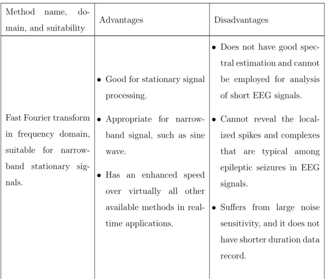
Table 3.2: Comparison between performance of different EEG feature extraction methods.
Method name,
do-main, and suitability Advantages Disadvantages
Fast Fourier transform in frequency domain, suitable for narrow-band stationary sig-nals.
• Good for stationary signal processing.
• Appropriate for narrow-band signal, such as sine wave.
• Has an enhanced speed over virtually all other available methods in real-time applications.
• Does not have good spec-tral estimation and cannot be employed for analysis of short EEG signals.
• Cannot reveal the local-ized spikes and complexes that are typical among epileptic seizures in EEG signals.
• Suffers from large noise sensitivity, and it does not have shorter duration data record.
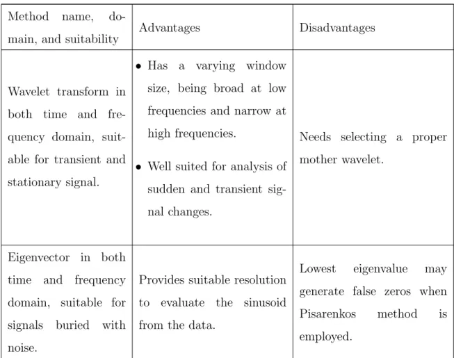
Table 3.2: continued
Method name, do-main, and suitability
Advantages Disadvantages
Wavelet transform in both time and fre-quency domain, suit-able for transient and stationary signal.
• Has a varying window size, being broad at low frequencies and narrow at high frequencies.
• Well suited for analysis of sudden and transient sig-nal changes.
Needs selecting a proper mother wavelet.
Eigenvector in both time and frequency domain, suitable for signals buried with noise.
Provides suitable resolution to evaluate the sinusoid from the data.
Lowest eigenvalue may generate false zeros when Pisarenkos method is employed.
Table 3.2: continued
Method name, do-main, and suitability
Advantages Disadvantages
AR in frequency do-main, suitable for sig-nal with sharp spec-tral features.
• Limits the loss of spec-tral problems and yields improved frequency reso-lution.
• Gives good frequency res-olution.
• Spectral analysis based on AR model is particularly advantageous when short data segments are ana-lyzed, since the frequency resolution of an analyti-cally derived AR spectrum is infinite and does not de-pend on the length of an-alyzed data.
• The model order in AR spectral estimation is dif-ficult to select.
• Gives poor spectral esti-mation once the estimated model is not appropriate, and models orders are in-correctly selected.
• Is readily susceptible to heavy biases and even large variability.
3.4 Features classification
Generally, a good BCI system needs a good pattern identification and translation part, which depends on classification algorithms used in the system [19]. A classifi-cation algorithm is designed to train a system that can predict the class of an input data based on its features [85]. In other words, it finds out that a new observation
belongs to which sub-population or category. There are several factors that should be considered in choosing the classifier. An example of problems in classifications is the curse of dimensionality [21].
The curse of dimensionality is a concern when the training set is small but the dimensionality of the feature vector is high. The system needs enough data to describe the different categories and find the proper class for a newcomer signal. Depending on feature vector dimensionality, the required data will be increased exponentially [86]. For a good classification performance, it is suggested to have training samples more than at least five times rather than the features dimensionality [87].
3.4.1 Linear Discriminant Analysis (LDA)
Linear Discriminant Analysis (LDA) is a statistical pattern recognition and ma-chine learning method for classification problems. It is also used for dimensionality reduction before later classifications. LDA looks for a linear combination of variables, which can best describe data, and in this point of view it is similar to PCA [88, 89]. Two major advantages of LDA over PCA for some types (not all) of data are explained in the following.
PCA is based on the covariance matrix. Covariance in sensitive to individual large values, so if someone takes a single attribute of the data and multiplies it by a large number, the PCA will be easily messed up. It wrongly shows that large attribute as the dominant component of the whole data. The other problem with PCA is that it considers the space as a linear one, so that in one dimensional it finds a straight line and in two dimensional it finds a flat sheet.
Most times we use PCA to reduce dimensionality before classification problems. It sometimes helps but sometimes not. It can sometimes hurt the data preprocessing. A reason is that PCA only looks at the datapoint coordinates but does not consider the classes labels. As a result the dimension that it picks might be very bad for
later classifications. Take, for example, the data points in figure 3.5 3. There are
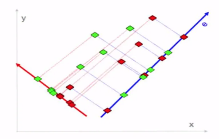
two classes of red and green. PCA takes the dimension with the greatest variance (dimension along the blue axis shown in the figure 3.5), and projects all the datapoint on this axis. This makes the two classes completely mixed into each others. There is no way to separate the data in new dimensions. However, if different dimension is picked up (like the red axis), then the projected data will be easily seperable. Hence, we need to find another way to choose a dimension as close as possible to this red axis. This is where LDA got introduced. LDA is a version of PCA that reduces the dimensionality in such a way that is most useful for the classifier [90].
Fig. 3.5: LDA versus PCA in finding a new axis for separation of red and green data. Both methods project the data on their new axis. LDA finds the red axes and PCA finds the blue one.
LDA is very similar to PCA, but it takes advantage of class labels when picking a new dimension. This new dimension gives maximum separation between means of projected classes, while having minimum variance within each projected class. LDA algorithm takes a few assumptions such as the data is Gaussian and there is a simple boundary between the data points. As result LDA does not always guarantee a
3linear discriminant analysis, Introductory Applied Machine Learning (IAML) course by Victor
better projection for the classifier. It usually fails when separating information is not in the mean of datapoint in each class, but is in the variance the data. So, generally, sometimes LDA works better (like in figure 3.64), sometimes PCA gives better result
(like in figure 3.7 5). They should be tried out in experiments.
Fig. 3.6: LDA works better than PCA in this case, because the mean of two datasets are easily distinguishable.
Fig. 3.7: PCA performs better than LDA in this case, because the means of two variables are very close to each other but their variance can distinguish them.
4linear discriminant analysis, Introductory Applied Machine Learning (IAML) course by Victor
Lavrenko at the University of Edinburgh
5linear discriminant analysis, Introductory Applied Machine Learning (IAML) course by Victor
3.4.2 Support Vector Machine (SVM)
In 1964, Vapnik and Chervonenkis introduced a new algorithm which constructs an optimal separating hyperplane when the training data is separable. They proposed the method with the simplest possible case, which is to have linear machines on separable data. At that time, they called it the generalized portrait method [91]. In 1995, Vapnik and Cortez generalized the method to a non-separable set of training data [92]. The concept of SVM is given in the following.
Considering that the problem is to divide positives from negatives in the figure 3.8, we are trying to find the line (plane and hyperplane in higher dimensions) that can separate the data into two groups. There can be many lines (planes or hyperplanes) to separate the training data into groups, but the question is which one is the best. According to [93], the best choice is the one that leaves the maximum margin from both classes. This is also called the widest approach because we are looking for the widest street that separates the positives from the negatives. As result, the SVM method tries to put the line in such a way that the street is as wide as possible.
Fig. 3.8: Two classes of positives and negatives.
Vapnik tried to first find the decision rules that make that decision boundary. Imagine that we have a vector ¯w of any length perpendicular to the median line of the street and also an unknown vector ¯u. The question is to figure out the vector ¯uis on which side of the street. To find the answer, we would need to find the distances
Fig. 3.9: Widest possible street between closest elements of two groups.
of ¯u with any lines of the street. So that we project the vector ¯u onto a vector that is perpendicular to the street, like ¯w. The starting point is to is to see if the inner product of ¯w and ¯u is greater than a constantc or not.
¯
w·u¯≥c
For our positive-negative example, if the equation above is true, then the vector ¯u shows a positive sample. The dot product lets us apply the directional growth of one vector to another, and can give us the projection of ¯u on the ¯w. If we take b = −c, without loss of generality we can write our first decision rule for positive samples as:
¯
w·u¯+b≥0 (3.7)
The equation 3.7 is not specific, because there can be many b and ¯w. In order to fix a particular b and ¯w there should be more constraints. Let’s take the inner product of ¯w with a positive sample x+ that is on the positive side of the street, we
will have the equation:
¯
w·x¯++b≥1
Likewise if take the inner product of ¯w with a negative sample x− that is on the
negative side of the street, we can we will have the equation: ¯
Since dealing with two equations is not mathematically convenient, we can intro-duce a new variable yi such that,
yi =−1 for negative samples
yi = +1 for negative samples
where the value of y show that in which group our sample is. Multiplyingyi with the
decision rules, we will have both equations equal to a single equation defined as: yi( ¯w·x¯i+b)≥1 or
yi( ¯w·x¯i+b)−1≥0
It is equal to zero (= 0) for xi on the borders of the street. So the second decision
rule can be:
yi( ¯w·x¯i+b)−1 = 0 for xi on the borders of the street. (3.8)
Fig. 3.10: Vector of deference of positive support vector and negative support vector. The dot product of this vector and a normal unit vector gives the width of the street.
At this point we can have the vector for the negative and the vector for the positive samples on the border. The dot product of the vector (¯x+−x¯−) and a normal unit
vector, gives us the width of the street in figure 3.10. We have assumed that ¯w is a normal, so ||ww¯|| is a normal unit vector.
width= (¯x+−x¯−)·
¯ w
||w|| (3.9)
From equation 3.8 for x+ (positive samples) yi = 1 and for x− (negative samples)
yi =−1 so that, x+.w¯= 1−b x−.w¯=−1−b
substituting these values for in the equation 3.9:
width= (¯x+−x¯−)· ¯ w ||w|| = 1−b−(−1−b) ||w|| = 2 ||w|| (3.10)
Considering the equation 3.10, in order to maximize the width of the street, ||w2|| should be maximized. We can instead minimize ||w||, which means we can solve the following optimization problem:
minimize 12(||w||)2
subject to yi( ¯w·x¯i+b)−1 = 0 f or i = 1,2,3,· · · , N
(3.11)
The method of Lagrange multiplier is used to find the minimum of the function in equation 3.11. Generally the Lagrange multiplier method (introduced by Joseph Luis Lagrange) is a strategy that is used in optimization problems to find the local minimum or maximum of a function by putting the main function and the constraints in a single equation [94, 95]. As result, the Lagrange multiplier method gives us a new expression (L) that can be maximize or minimize without thinking about the constraints any more. L is the function minus the summation of constraints while each constraint is equal to 0 and has a multiplier.
L= 1 2||w||
2−X
i
αi[yi( ¯w·x¯i+b)−1] (3.12)
We are minimizing L in respect to variables ¯w and b. Because the differentiating in respect to a vector is same as the differentiation in respects to a scalar, the extremum of L is easy by finding the derivatives in respect to all variables and set them to 0.

![Fig. 3.2: 10-20 standard system [34].](https://thumb-us.123doks.com/thumbv2/123dok_us/859383.2609578/36.918.262.711.109.367/fig-standard-system.webp)
![Fig. 3.3: 10-20 system modified by American EEG society [34].](https://thumb-us.123doks.com/thumbv2/123dok_us/859383.2609578/37.918.320.633.114.427/fig-modified-american-eeg-society.webp)