Understanding Exchange Rate Dynamics: What Does
The Term Structure of FX Options Tell Us?
Yu-chin Chen and Ranganai Gwati
∗March 2014
Abstract
This paper proposes using foreign exchange (FX) options with different strike prices and maturities (“the term structure of volatility smiles”) to capture both FX expectations and risks. Using daily options data for six major currency pairs, we show that the cross section and term structure of options-implied standard deviation, skewness and kurtosis consistently explain not only the conditional mean but also the entire conditional distribution of subsequent currency excess returns for horizons ranging from one week to twelve months. This robust empirical pattern is consistent with a representative expected utility maximizing investor who, in addition to caring about the mean and variance, also cares about the skewness and kurtosis of the return distribution. We also find that exchange rate movements, which are notoriously difficult to model empirically (“the exchange rate disconnect puzzle”), are in fact well-explained by the term structures of forward premia and options-implied higher moments. Our results suggest that the perennial problems faced by the empirical exchange rate literature are most likely due to overly restrictive assumptions inherent in prevailing testing methods, which fail to properly account for the forward-looking property of exchange rates and potential skewness or excess kurtosis in the conditional distribution of FX movements.
Keywords: exchange rates; excess returns; options pricing; volatility smile; risk; term structure of implied volatility; quantile regression
JEL Code: E58, E52, C53,F31,G15
∗First Draft:October 2012. We are indebted to the late Keh-Hsiao Lin and Joe Huang for pointing
us to the relevant data sources. We would also like to thank Samir Bandaogo, Nick Basch, Yanqin Fan, David Grad, Ji-Hyung Lee, Charles Nelson, Bruce Preston, Abe Robison, and Eric Zivot for their helpful comments and assistance. All remaining errors are our own. Chen’s and Gwati’s research are supported by the Gary Waterman Scholarship and the Buechel Fellowship at the University of Washington. Chen: [email protected]; Gwati: [email protected]; Department of Economics, University of Washington, Box 353330, Seattle, WA 98195
1
Introduction
The exchange rate economics literature has over the years faced many empirical “puzzles”, or anomalies that are hard “to explain on the basis of either sound economic theory or practical thinking” Sarno (2005). As an example, although theory predicts that nominal exchange rates should depend on current and expected future macroeconomic fundamentals, the consensus in the literature is that exchange rates are essentially empirically “disconnected” from the macroeconomic variables that are supposed to determine them. This empirical disconnect comes in the form of low correlations between nominal exchange rates and their supposed macro-based determinants and also in the form of poor performance of macro-based exchange rate models in out-of-sample forecasting (see Engel (2013) for a review).
A related empirical anomaly that has received considerable attention in the literature is the uncovered interest parity (UIP) puzzle or the forward premium puzzle. The UIP puzzle is the empirical irregularity showing that the forward exchange rate is a biased predictor of future spot exchange rates. One manifestation of this empirical (ir) regularity is that countries with higher interest rates tend to see their currencies subsequently appreciate and a “carry-trade” strategy exploiting this pattern, on average, delivers excess currency returns.1 This violation of the UIP condition is commonly attributed to time-varying
risk premia and biases in (measured) market expectations. However, empirical proxies based on surveyed forecasts or standard measures of risk - for instance, ones built from consumption growth, stock market returns, or the Fama and French (1993) factors - have been unsuccessful in explaining the puzzle. 2 As such, while recognizing the presence of risk, macroeconomic-based approaches to modeling exchange rates often ignore risk in empirical testing ( see for instance, Engel and West (2005); Mark (1995)). On the finance 1 A carry trade strategy is to borrow low-interest currencies and lend in high-interest currencies, or to
sell forward currencies that are at a premium and buy forward currencies with a forward discount.
2 See, Engel (1996) for a survey of the forward premium literature, as well as recent studies such as
side, efforts aiming to identify portfolio return-based “risk factors” offer some empirical success in explaining the cross-sectional distribution of excess FX returns, but have little to say about bilateral exchange rate dynamics (see for example, Lustig et al. (2011); Menkhoff et al. (2012); Verdelhan (2012)). 3 The UIP puzzle is taken seriously in the exchange rate
literature because the UIP condition is a property of most open-economy macroeconomic models.
This paper first links the persistent empirical puzzles faced by the exchange rate economics literature to overly restrictive preference and distributional assumptions in conventional testing methods. We argue that these auxiliary assumptions often inadequately account for either the forward-looking property of nominal exchange rates or potential skewness and/or fat tails in the distribution of FX returns. We then propose using the term structure of volatility smiles to capture expectations of future macroeconomic conditions as well as market perceived volatility, crash and tail risk of future exchange rate realizations.
Conceptually, since payoffs of option contracts depend on the uncertain future realization of the price of the underlying asset, option prices must reflect market sentiments and beliefs about the probability of future payoffs. Using prices of a cross section of option contracts (at-the-money, risk reversals and vega-weighted butterflies at 10 and 25 deltas) which deliver payoffs under differential future realizations of the spot exchange rate, we uncover ex-ante standard deviations, skewness, and kurtosis of the distribution of expected future exchange rate movements.
With daily options data for six major currency pairs and seven tenors, we show that these market-based ex-ante measures of FX volatility, crash and tail risk can explain the conditional means of excess currency returns or ex-post deviations from UIP for horizons ranging from one week to twelve months. We then use quantile regression analysis to demonstrate that 3Lustig et al. (2011) and Verdelhan (2012) for example, identify a “carry factor” based on cross sections
of interest rate-sorted currency returns and a “dollar factor” based on cross sections of beta-sorted currency returns.
the options-based FX risk measures not only explain the conditional mean but also the entire conditional distribution of subsequent deviations from UIP . Additionally, we find that proxies for options-implied FX global risks show significant explanatory power for quarterly excess returns.
We carry out a battery of robustness checks that include robust least squares regression analysis, regression analysis using non-overlapping data and option-implied moments extracted from 10-delta options (instead of the 25-delta options used in the main regressions) as well as sub-sample analyses. Our main empirical findings survive these robustness tests, suggesting that the strong empirical relationship between excess returns and options-based measures of FX higher moment risks is not being driven by issues such as our use of data with overlapping observations or the presence of outliers in our sample.
We then move beyond matched-frequency analysis and extend the approach pioneered by Hansen and Hodrick (1980) and later used in Clarida and Taylor (1997) and Chen and Tsang (2013), that uses the forward rates or interest differentials over time and across currency pairs to model excess returns. The term structure component adds significant explanatory power, shown by the huge increases in the adjusted R2s when compared to results from matched frequency analyses.4
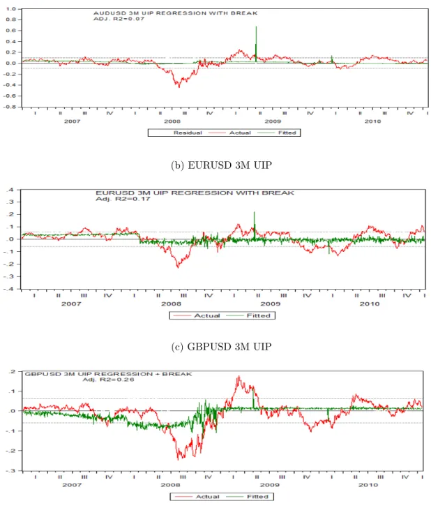
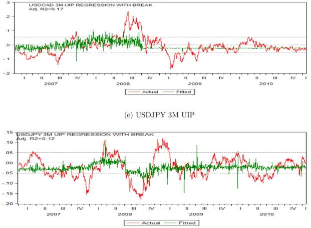
We further show that exchange rate movements, which have proved notoriously hard to model empirically over the years, are in fact well-explained by the term structures of option-implied first moments and higher order moments. Standard UIP analyses regress exchange rate movements on the first moment of the perceived distribution of exchange rate movements for the same tenor, and the explanatory power of such are usually very low. For quarterly exchange rate movements, we find that augmenting such regressions by also including information from the term structure of first moments as well as the term structure of option-implied second to fourth moments yields R2s ranging from 70% to 85% and fit
remarkably well. The good fit of our multi-moment term structure specifications, shown in figures (4a)-(4e), can be contrasted to the poor fit of the standard UIP regressions shown in figures (5a)-(5e).
On one hand, there is a huge literature linking the term structure of interest rate rates (or yield curve) to expected future dynamics of macroeconomic fundamentals such as monetary policy, inflation and output (for example, Ang and Piazzesi (2003), Diebold et al. (2006) and Ang et al. (2006)). Chen and Tsang (2013) extend this strand of literature to the open economy context by noting that the term structure of interest rate differentials (relative yield curve) contain information about the expected future dynamics of differences in macroeconomic fundamentals. On the other hand, we argue in section (2) that the term structure of option-implied first moments captures the same information as the term structure of interest rate differentials. Therefore, to the extent that the relative yield curve contains information about expected future path of domestic and foreign macroeconomic conditions, our findings that the term structure of first moments help explain exchange rate movements suggest that exchange rates are not disconnected from macroeconomic fundamentals. On one hand, studies that focus on term structure dynamics tend to only concentrate on forward exchange rates or interest rate differentials, which are first moments of the distributions of future spot rates (for example Hansen and Hodrick (1980), Clarida and Taylor (1997) and Chen and Tsang (2013)). On the other hand, studies that focus on higher moment risks tend to conduct matched-frequency analyses (for example, Malz (1997) and Lyons (1998)).
The robust empirical findings in this paper suggest that both expectations and risk should be carefully accounted for in structural and empirical modeling of exchange rates. In addition, our results suggest that over-the-counter FX options market captures both concepts in practice. These results also demonstrate that the perennial problems faced by the exchange rate economics literature are most likely due to overly restrictive auxiliary assumptions in
the empirical testing of the models rather than to limitations of the theoretical models themselves.
Simple derivatives such as the forwards and futures have been used extensively in explaining excess currency returns or exchange rate movements.5 Payoffs from forward contracts,
however, are linear in the return on the underlying currency and as such do not contain as useful a set of information as the non-linear contracts we examine. Indeed, FX options have been used to proxy variance or tail risk in various specific contexts such as testing the portfolio balance model of exchange rate determination (Lyons (1998)), measuring announcements effects (Grad (2010)), evaluating rare events theory (Farhi et al. (2009)) and conducting density forecasts (Christoffersen and Mazzotta (2005)). To the best of our knowledge, however, there has been no systematic and comprehensive testing of whether the ex-ante information contained in the term structure of volatility smiles indeed predicts ex-post excess currency returns. Our paper aims to bridge this gap. 6
Our use of options price data and related empirical methodologies has a number of motivating factors. First, options are forward-looking by construction, which means option prices should therefore be able to incorporate information such as forthcoming regime switches or the presence of a peso problem.7 Second, option prices are deeply rooted in market participant behavior because they are based on what market participants do instead of what they say. 8 Furthermore, cross sections of option prices imply a subjective probability
5See for example, Hansen and Hodrick (1980) and Clarida and Taylor (1997) among many others. 6 This paper also contributes more generally to bridging the gap between the literature on currency
derivative pricing and that on the economics of exchange rates. Chen (1998) comments that “Most students of financial economics focus on the mathematical tools of the option pricing models with little emphasis on the economics of exchange rate determination, while traditional macro-international economics tend to shy away from the technicality of the currency derivative, despite its obvious importance in practice. This gap in academic research and training has created a problem for practitioners” .
7 The peso problem refers to the effects on inferences caused by low-probability events that do not occur
in the sample, which can lead to positive excess return.
8As discussed earlier, forward contracts are forward-looking by construction, but for a given currency
pair and tenor, there is only one forward price with linear dependency on future spot realization. The multiple option prices for options with different strikes offer a much richer information set. Lastly, standard constructions of market expectations and perceived risks based on macro fundamentals or finance factors do not work well.
distribution of future spot exchange rates, which captures both market participants’ beliefs and preferences. 9Third, modern techniques such as the Vanna-Volga method (see Castagna and Mercurio (2005)) and the methodology of Bakshi et al. (2003) facilitate elegant and model-free computation of options-implied higher order moments of future exchange rate changes. Lastly, option-implied moments can be extracted at a higher frequency, the options approach gives us genuinely conditional estimates and avoids a trade-off problem encountered when estimating higher moments from historical returns data. When using historical returns data, longer windows are required to increase precision, while shorter windows are required to obtain conditional rather than unconditional estimates.
2
Why Higher Order Moments and Term Structure?
2.1
Forward Premium Puzzle and Excess Currency Returns
The efficient market condition for the foreign exchange markets, under rational expectations, equates cross border interest differentials it−i∗t with the expected rate of home currency
depreciation, adjusted for the risk premium associated with currency holdings, ρt:10
iτt −iτ ,t ∗ =Et∆st+τ +ρt+τ. (2.1)
This condition is expected to hold for all investment horizons τ, with interest rates that are at matched maturities. Ignoring the risk premium term, numerous papers have tested this 9This distribution is commonly referred to as the “risk-neutral distribution”, though it does NOT
imply that the distribution is derived under risk-neutrality. On the contrary, it incorporates both the expected physical probability distribution of future exchange rate realization as well as the risk premium, or compensation required to bear the uncertainty.
10 In this paper, we define the exchange rate as the domestic price of foreign currency. A rise in the
exchange rate indicates a depreciation of the home currency. However, “home”does not have a geographical significance but follow the FX market conventions. See table (1A)
equation since Fama (1984), and find systematical violations of this UIP condition: st+τ −st =α+β(iτt −i ∗,τ t ) +t+τ; Et[t+τ] = 0,∀t, H0 :β = 1 (2.2)
with an estimated β < 0 and R2s that are usually close to zero. This is the so-called uncovered interest rate parity puzzle or the forward premium puzzle (see Engel (1996), for a survey of the literature). To see the connection with forward rates, we note that the covered interest parity condition, an empirically valid no-arbitrage condition, equates the forward premiumftt+τ−st,with interest differentials. The risk-neutral UIP condition above
thus implies that the forward rate should be an unbiased predictor for future spot rate: Etst+τ =ftt+τ or st+τ =ftt+τ +ut+τ,where Et[ut+τ] = 0∀t.
We should next define FX excess returns as the rate of return across borders net of currency movement, and one can see that the UIP or forward premium puzzle can be expressed as a non-zero averaged excess return over time:
xrt+τ =ftt+τ −st+τ = (iτt −i τ ,∗
t )−∆st+τ =ρt+τ +ut+τ (2.3)
It is natural then to note that the empirical failure of the risk-neutral UIP condition can be attributable to either the presence of a time-varying risk premium, ρt+τ, or that expectation error, ut, may not be i.i.d. mean zero over time. If the distribution of either of these is
not mean zero over the time series, empirical estimates of the slope coefficient in regression equation (2.2) would likely suffer omitted variable bias or other complications.
2.1.1 Some issues with conventional tests of UIP
The forward unbiasedness hypothesis is true for a given distribution of st+τ at each point in
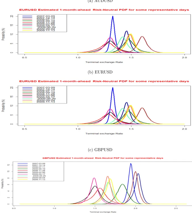
the extracted option-implied moments and sample distributions in figure ( 1) below - then testing the hypothesis Etst+τ = ftt+τ using time series data might not be appropriate. The
OLS regression-based testing framework in equation (2.2) makes the auxiliary assumption that shocks to ∆st+τ are i.i.d. normal over time. However, FX returns are well documented
to have fatter tails than normal, and in some cases skewed. 11
INSERT FIGURE (1) HERE
2.2
Why higher order moments?
12In this subsection we show that in addition to risk neutrality and rational expectations assumptions, the UIP condition also hinges on the rather restrictive auxiliary assumptions that FX returns are i.i.d. normal over time and that investors have constant absolute risk aversion (CARA) utility. These two additional assumptions reduce the representative investor’s optimal asset allocation problem to a mean-variance optimization problem.
We start with the problem of an investor who, in each period, allocates her portfolio among risky assets with the goal of maximizing the expected utility of next period wealth. In each period, the investor hasn risky assets to choose from. The vector of gross returns is given byrt+1 = (r1,t+1, ..., rn,t+1). If we supposeWtis arbitrarily set to 1, thenWt+1 =α
0 trt+1
, where α is an n by 1 vector of portfolio weights.
The investors problem is to choose αt to maximize the expression
Et[U(Wt+1)] =Et[U(α 0 trt+1)]
=R ...R U(Wt+1)f(rt+1)dr1,t+1dr2,t+1...drn,t+1
(2.4)
11Cincibuch and Vavra (2004) write: “It is common knowledge that financial returns are not normal, that
they usually have heavy tails and that they might be skewed. Therefore it seems odd to test efficiency, which involves the notion that rational market players utilize all available information, and restrict the expectation error to be normal. ”
subject to the condition thatPn
i=1αi,t = 1, wheref(rt+1) is the joint probability distribution
of rt+1.
2.2.1 CARA and Normality reduce problem to mean-variance optimization
Let us further assume that the investor has CARA utility and that returns are conditionally normally distributed. The CARA utility assumption means the utility is given by
U(Wt+1) = −e−γWt+1 , where γ ≥ 0 is the coefficient of absolute risk aversion. The
distributional assumption rt+1 ∼N(µt+1,Σt+1) implies that Wt+1 ∼N(µp,t+1, σ2p,t+1), where
µp,t+1 =α0tµt+1 and σ2
p,t+1 =α
0
tΣt+1αt
With the above two assumptions, expression (2.4) reduces to13
Et[U(Wt+1)] = −Et[e−γWt+1] =γµp,t+1−
1 2γ
2σ2
p,t+1 (2.5)
Equation (eq:MVOptim) demonstrates that under the assumptions of CARA utility function and conditional normality of returns, the general portfolio allocation problem (2.4) reduces to the mean-variance optimization problem.14
If we further assume that our investor has a 2-asset portfolio made up of a nominally safe domestic bond and a foreign bond, and that she allocates a fraction α of her wealth to the domestic bond, then next period wealth expressed in local currency units is given by
Wt+1 = α(1 +it) + (1−α)(1 +i∗t) St+1 St. Wt (2.6)
In this 2-asset example and CARA utility and conditionally normal returns the expressions 13The second equality follows from the fact that e−γWt+1 ∼ LN(−γµ
p,t+1, γ2σ2p,t+1) , so Et[e−γWt+1] =
−γµp,t+1+γ2σ2p,t+1
14The quadratic utility function imply mean variance optimization for arbitrary return distribution.
However, the quadratic utility implies increasing absolute risk aversion and satiation (Jondeau et al. (2010), page 352).
for the conditional mean and variance of next period wealth are given by: µp,t+1 = h α(1 +it) + (1−α)(1 +i∗t)E tSt+1 St i Wt, σ2 p,t+1 = (1−α)2(1+i∗ t)2V art(St+1)Wt2 S2 t (2.7)
Plugging the expressions in equation (2.7) into objective function (2.5), taking the first order condition with respect toαand rearranging the first order condition yields the following equation which implicitly determines the optimal α:
(1 +it)−(1 +i∗t) EtSt+1 St = −γWt(1−α)(1 +i ∗ t)2V art(St+1) S2 t . (2.8)
Equation (2.8) reduces to the UIP condition if we assume that all investors are risk-neutral (γ = 0):15 1 +it 1 +i∗t = EtSt+1 St . (2.9)
The Fama regression in equation (2.2) tests a logarithmic version of equation (2.9). The key steps in deriving the testable restrictions in equation (2.9) are the joint assumptions of CARA utility and conditional normality of next period wealth, which reduce the investor’s optimization to mean-variance. The above discussion illustrates that deriving the UIP equation tested through expression (2.2) depends on other assumptions beyond rational expectations and risk-neutrality. If the normality assumption is dropped, for example, then expression (2.9) will most likely include higher order moments. In fact, Jondeau et al. (2010) note that under CARA utility, if we drop the normality assumptions, then the investor would prefer positive skewness and low kurtosis, such that the investor’s objective function in equation (2.5) will also include the third and fourth moments of the FX return distribution. Scott and Horvath (1980) show that a strictly risk-averse individual who always prefers more to less (U(1) >0) and likes positive skewness at all wealth levels will necessarily dislike high
kurtosis.
2.3
Why term structure?
The term structure of option prices allows us to extract information about expected future macroeconomic conditions. Going back to UIP equation (2.1), rearranging and iterating forward, one can show that the nominal exchange rate depends on current and expected future interest rate differentials as well as on expected risk. The interest rates are monetary policy variables, and thus depend on macroeconomic fundamentals.
st= − ∞ X j=0 Et(it+j −i∗t+j) | {z }
Expected future interest differentials
− ∞ X j=0 Etρt+j | {z }
Expected Future FX risk
(2.10)
Writing the exchange rate in the form in equation (2.10) demonstrates the importance of capturing expectations and risks in testing exchange rate models. Standard empirical approaches, however, impose distributional assumptions that reduce the sum of expected future fundamentals to equal current fundamentals and also ignore risk (see Engel and West (2005), Mark (1995)).
Chen and Tsang (2013) propose using information contained in the term structure of interest rate differentials to side-step these distributional assumptions. They exploit information in the term structure of relative interest rate differentials to proxy for expected changes in future macro fundamentals and show that Nelson and Siegel (1987) factors extracted from relative yield curves predict bilateral FX returns and explain excess currency returns one month to two years ahead. Clarida and Taylor (1997) and Clarida et al. (2003) show that even if the forward rate is a biased predictor of future spot rate (the forward premium puzzles), the term structure of forward premia still contains information useful for predicting subsequent exchange rate changes.
of capturing expectations. We propose to use information contained in the term structure of option prices to capture the first part of (2.10) and use the cross section of option prices to capture the expected risk component. In subsection (3.1), we argue that the term structure of volatility smile contains information about expected future macro conditions and FX risks
beyond that contained in either the relative yield curve or term structure of forward premia.
3
Information Content of Currency Options
Option prices provide (at least) three distinct pieces of information about market participants’ expectations and preferences: options with the same underlying currency pair and tenor but different strike prices (volatility smile), options with the same strike price and same underlying currency pair but different tenors (term structure of implied volatility) and lastly, prices of options with the same strike price tenor but different underlying currency pairs. In section (3) we explain the information theoretically contained in the volatility smile, term structure of option prices and cross correlations of option prices with different underlying currency pairs. We then describe a methodology for extracting this information.
3.1
Volatility Smile, Term Structure and Cross Correlations
Breeden and Litzenberger (1978) show that in complete markets, the call option pricing function (C) and the exercise price K are related as follows:
∂2C ∂K2 =e
−rdτπQ
t (St+τ), (3.1)
where rd and rf are the domestic and foreign risk-free interest rates and πQ
t(St+τ) is the
risk-neutral probability density function (pdf) of future spot rates. Equation (3.1) implies that, in principle, we can estimate the whole pdf of time St+τ spot exchange rate from time
estimates of the standard deviation, skewness , kurtosis and even higher order moments of the market perceived probability density of St+τ given information available at timet.
In addition to the Breeden and Litzenberger (1978) result in equation (3.1), we note that although market participants can be treated as if they are risk-neutral for the purpose of option-pricing, option prices theoretically contain information about both investor beliefs and risk preferences, as shown from the following formula for the price of a European-style call option: C(t, K, T) = Z ∞ K Mt,T(ST −K) | {z } Preferences πPt (ST) | {z } Beliefs dST =e−r dτZ ∞ K (ST −K)πQt (ST) | {z } Both dST. (3.2)
In equation (3.2),Mt,t+τ is the pricing kernel, which captures the investor’s degree of risk
aversion and πP
t(St+τ) is the physical probability density function of future spot exchange
rates 16.
A forward contract can in fact be viewed as a European-style call option with a strike price of zero. To see this, we recall that, on one hand, the theoretical forward exchange rate is given by the formula:
Ft,T =e−r dτZ ∞ 0 STπQt (ST)dST =e−r dτ EQt(ST). (3.3)
On the other hand, evaluating equation (3.2) at K=0 yields:
C(t,0, T) = e−rdτ Z ∞ 0 STπ Q t(ST)dST =Ft,T. (3.4)
The relationship between options and forwards in equation (3.4) suggests that the cross section of option prices should, at a minimum, contain as much information about investor beliefs and preferences as that contained in forward prices.
16 In the second expression, the pricing kernel is performing both the risk-adjustment and discounting
Moving on to the term structure of option prices, one way to motivate the theoretical information content of the term structure of option prices is to start from equation (2.10):
st = − ∞ X j=0 Et(it+j−i∗t+j) | {z }
Expected future interest differentials
− ∞ X j=0 Etρt+j | {z }
Expected Future FX risk
. (3.5)
Now, under the empirically valid CIP condition, interest rate differential is equal to the forward premium for all tenors j:17
it+j−i∗t+j =f t+j t −st=−rdτ +EtQ ln St+j St | {z } First moment ofπQt + ωt |{z}
Jensen’s inequality term
,∀ tenor j. (3.6)
Equation (3.6) thus says that, ignoring the Jensen’s inequality termωtand the constant
term −rdτ, the interest rate differential equals the first moment of the option-implied
risk-neutral distribution of lnSt+j
St
for any given tenorj. The interest rates are monetary policy variables and therefore depend on macroeconomic fundamentals such as unemployment and inflation. When combined, equations (3.6) and (3.5) demonstrate that just like the yield curve, the term structure of the first moments of implied distributions also captures information about current and expected future macroeconomic fundamentals.
A second motivation for the information content of the term structure of option prices comes from the expectation hypothesis for implied volatility. If the expectations hypothesis holds in the FX market, then the implied volatility for long dated options should be consistent with the implied volatility of short dated options quoted today and in the future. For example, if the current six month implied volatility is 10% and the current three month implied volatility is 5%, then, under the expectation hypothesis, then the three month implied
17The second equality follows from dividing (3.3) by S
volatility three months from now should be 13.2% because
0.5(0.1)2 = 0.25(0.05)2+ 0.25(0.132)2.
The expectation hypothesis therefore suggests that the term structure of option-implied volatility contain information about the market’s perception about the future dynamics of short term implied volatility. Starting from the Hull and White (1987) stochastic volatility model, Campa et al. (1998b) test the expectation hypothesis for FX implied volatility and fail to reject the hypothesis.
A third source of information from currency options is by using correlations of options on different currency pairs to construct global measures of FX risk. Option-implied correlations arise from three way arbitrage arguments. For example: if the exchange rates at time t are given bySAB,t, SAC,t andSBC,t and assuming they follow stationary processes, we have that
ln(SAB,t) =ln(SAC,t)−ln(SBC,t) = sAC,t−sBC,t (3.7)
Equation (3.7) above implies that
V art(sAB) = V art(sAC) +V art(sBC)−2Corrt(sAC, sBC)V art(sAC)
1
2V art(sBC) 1
2, (3.8)
which can be rearranged to give:
Corrt(sAC, sBC) = V art(sAC) +V art(sBC)−V art(sAB) 2V ar 1 2 t(sAC)V art(sBC) 1 2 (3.9)
If we use option-implied variance to estimate the right hand side of equation (3.9), then the resulting estimate of ρt(sAC, sBC) is option-implied correlation. Siegel (1997) points
out that this option-implied correlation reveals market sentiment regarding how closely the currencies are expected to move in the future. The average option-implied correlation can
be interpreted as capturing global FX correlation risk.
Recently, efforts aiming to identify portfolio return-based global “risk factors” offer some empirical success in explaining the cross-sectional distribution of excess FX returns. 18 19 The majority of existing research in this line of literature, however, use proxies of global risk constructed from historical returns and focus on matched-frequency analysis. Given the advantages of using option price data outlined in section (1), a natural question to ask is whether options-based measures of FX global risk add further insights to the strand of literature using global FX risk to explain FX excess returns and FX returns.
3.2
Extracting Option-Implied Moments
20We use the methodology of Bakshi et al. (2003) (henceforth BKM) to extract model-free option-implied standard deviation, skewness and kurtosis from the volatility smile. Grad (2010) and Jurek (2009) also use the BKM methodology to extract FX options-implied higher order moments. 21
The extracted moments using the BKM methodology are model-free because we make no assumptions regarding the time series process governing the underlying spot exchange rate. The model-free nature of the methodology is attractive because it means the methodology is equally applicable to all exchange rate regimes. Campa et al. (1998a) argue that having a methodology that does not presuppose a stochastic process followed by the underlying spot exchange rate is especially useful in situations where the FX regime is unknown or changing, 18Verdelhan (2012)and Lustig et al. (2011) , for example, identify a “carry factor” based on cross section
of interest rate-sorted currency returns, and a “dollar factor” based on cross-section of beta-sorted currency returns. Rafferty (2011) constructs a global skewness risk factor using historical returns from carry trade portfolios and shows that higher average excess returns co-vary more positively with global skewness.
19 Menkhoff et al. (2012) investigate the role of global volatility risk in explaining cross-sections of carry
trade returns, and conclude that carry trade returns are compensation for exposure to global volatility risk. Mueller et al. (2012) investigate the role of global correlation risk as a driver of currency returns. Cenedes et al. (2012) show that higher average is significantly related to large future carry trade losses, while lower average correlation is significantly related to large gains.
20Extraction of moments done in the R statistical language R Core Team (2013). 21In this section we closely follow the exposition and notation in Grad (2010).
or when the degree of government intervention is unclear. The BKM methodology rests on the results of Carr and Madan (2001), which show that if we have an arbitrary claim with a pay-off function H[S] with finite expectations, then H[S] can be replicated if we have a continuum of option prices. They also show that if H[S] is twice-differentiable, then it can be spanned algebraically by the following expression
H[S] = (H[ ¯S] + (S−SH¯ S[ ¯S]) + Z ∞ ¯ S HSS[K](S−K)++ Z S¯ 0 HSS[K](K−S)+dK, (3.10) where HS = ∂H∂S and HSS = ∂ 2H
∂S2. Assuming no arbitrage opportunities, the price of a claim with pay-off H[S] is given by the expression
pt= (H[ ¯S]−SH¯ S[ ¯S])e−r dτ +HS[ ¯S]Se−r dτ + Z ∞ ¯ S HSS[K]C(t, τ , K)+ Z S¯ 0 HSS[K]P(t, τ , K)dK (3.11) where K is the strike price, C(t, τ , K) and P(t, τ , K) are, respectively, the prices of a European-style call and put options. ¯S is some arbitrary constant, usually chosen to equal current spot price.
Equation (3.11) indicates that any pay-off function H[S] can be replicated by a position of (H[ ¯S]−SH¯ S[ ¯S]) in the domestic risk-free bond, a position of H[ ¯S] in the stock, and
combinations of out-of-the-money calls and puts, with weights HSS[K]. Suppose we have
contracts with the following pay-off functions:22
H[S] = [Rt(St+τ)]2, Volatility Contract [Rt(St+τ)]3, Cubic Contract [Rt(St+τ)]4, Quartic Contract, (3.12) where Rt(St+τ) = ln(StS+τ t
. BKM show that the variance, skewness and kurtosis of the 22One can use the framework to price contracts with higher order payoffs and therefore extract moments
of order higher than 4. The point that we want to emphasize, that higher order moments matter, is demonstrated even if we only stop at 4thorder.
distribution of Rt+τ can be calculated using the following formulas: Stdev(t, τ) =perdτ V(t, τ)−µ(t, τ)2 (3.13a) Skew(t, τ) = erdτW(t,τ)−3V(t,τ)µ(t,τ)erdτ+2µ(t,τ)3 [erdτV(t,τ)−µ(t,τ)2]32 (3.13b) Kurt(t, τ) = erdτX(t,τ)−4erdτµ(t,τ)W(t,τ)+6erdτµ(t,τ)2V(t,τ)−3µ(t,τ)4 [erdτV(t,τ)−µ(t,τ)2]2 , (3.13c) where the expressions for V(t, τ),W(t, τ) and X(t, τ) andµ(t, τ) are given in appendix (A). Derivations of equations in (3.13) and expressions forµ(t, τ), V(t, τ), W(t, τ) andX(t, τ) can be found in Bakshi et al. (2003) and Grad (2010).
The BKM methodology described above requires a continuum of exercise prices. However, in the OTC FX options market implied volatilities are observed for only a discrete number of exercise prices. We therefore need a way to estimate the entire volatility smile from a few (K−σ) pairs by interpolation and extrapolation. To this end, we use the Vanna Volga (VV) method described in Castagna and Mercurio (2007). The procedure allows us to build the entire volatility smile using only three points. Castagna and Mercurio (2007) note that if we have three options with implied volatilityσ1,σ2,σ3 and corresponding exercise pricesK1,K2
and K3 such that K1 < K2 < K3, then the implied volatility of an option with arbitrary
exercise price K can be accurately approximated by the following expression:
σ(K) = σ2+ −σ2+ p σ2 2+d1(K)d2(K)(2σ2D1(K) +D2(K)) d1(K)d2(K) , (3.14) where D1(K) = lnK2 K lnK3 K lnhK2 K1 i lnhK3 K1 iσ1+ ln h K K1 i lnK3 K lnhK2 K1 i lnhK3 K2 iσ2+ ln h K K1 i ln h K K2 i lnhK3 K1 i lnhK3 K2 iσ3−σ2,
D2(K) = lnK2 K lnK3 K ln h K2 K1 i ln h K3 K1 id1(K1)d2(K1)(σ1−σ2) 2+ln[ K K1]ln[ K K2] ln[K3 K1]ln[ K3 K2] d1(K3)d2(K3)(σ3−σ2)2 and d1(x) = log[St x] + (r d−rf +1 2σ 2 2)τ σ2 √ τ , d2(x) =d1(x)−σ2 √ τ , x∈K, K1, K2, K3.
Expression (3.14) allows us to find the implied volatility of an option with an arbitrary strike price. We use K1 =K25δp, K2 =KAT M and K3 =K25δc. The VV methodology has a
number of attractive features, which are explained in Castagna and Mercurio (2007). First, it is parsimonious because it uses only three option combinations to build an entire volatility smile. This is the minimum number that can be used if one wants to capture the three most prominent movements in the volatility smile: change in level, change in slope, and change in curvature.23 The VV method also has a solid financial motivation: Castagna and Mercurio
(2007) show that it is based on a replication argument in which an investor constructs a portfolio that, in addition to hedging against movements in the price of the underlying asset (δ = ∂C∂S), also hedges against movements in volatility of the underlying asset (V ega= ∂C∂σ). In situations where volatility is stochastic, it might be useful to construct portfolios that, in addition to hedging against changes in the price of the underlying asset, the investor also hedges against for the Vega(∂C∂σ), the Vanna (∂∂σ2C2) and the Volga (
∂2C
∂σ∂S) as might be necessary
in situations when volatility is stochastic.
3.3
Data Description
In the o-t-c market, the exchange rate is quoted as the “domestic” price of “foreign” currency, which means a fall in the reported exchange rate represents an appreciation of domestic currency. “Domestic” and “foreign” , however, do not have any geographic significance, but 23The ATM straddle, VWB and the Risk Reversal capture these movements. See discussions in Castagna
are in accordance to some market quoting conventions. Table (1A) contains details of the market quoting conventions for the six currency pairs that we use in this paper.
Compared to exchange-traded options, there are several advantages that come with using o-t-c data in our empirical analysis. First, most of the FX options trading is concentrated in the o-t-c market. This means o-t-c currency options prices are more competitive and therefore more likely to be representative of aggregate market beliefs compared to prices in the less liquid exchange market. Table (1C), obtained from the 2010 BIS Triennial Survey, shows that although the o-t-c options market is small relative to the overall FX market, it is very liquid and rapidly growing when we look at it in absolute terms.
[INSERT TABLE (1C) HERE]
A second advantage of using o-t-c option price data is that fresh options for standard tenors are quoted each day, making it possible to obtain a time series of FX option prices with constant maturities. This can be contrasted with exchange traded options, whose prices are quoted for a specific expiry date, such that as we approach the expiry date, the option prices also incorporate the fact that the tenor is changing. O-t-c options make it possible to disentangle term structure, cross-sectional and time series aspects embedded in option prices.
Our third and final motivation for o-t-c option data is that European-style options are traded in this market, whereas exchange traded FX options are usually American-style. When analyzing option prices of a given tenor, American-style options have to be adjusted for the possibility of early exercise.
We next explain some important OTC currency market quoting conventions. First, option prices are given in terms of implied volatility instead of currency units while “moneyness” is measured in terms of the delta of an option. The delta of an option is a measure of the responsiveness of the option’s price with respect to a change in the price of the underlying asset. If the prices of call and put options are given by Ct and Pt, then option price
and implied volatility are linked using the formula from Garman and Kohlhagen (1983)’s extension of the Black-Scholes model to FX.
Ct = e−r dτ Ftt+τΦ(d1)−KΦ(d2) Pt = e−r dτ KΦ(−d2)−Ftt+τΦ(−d1) where d1 = log[St K] + (r d−rf +1 2σ 2 2)τ σ2 √ τ , d2 =d1−σ2 √ τ ,
There is a one-to-one relationship between option price and implied volatility when using the Black and Scholes (1973) formula. 24 The expressions for call and put deltas are given by the expressions: δc=e−r f Φ(d1) (3.15a) δp =e−r f Φ(−d1), (3.15b)
where Φ(.) is the standard normal cumulative density function (cdf). The absolute values of δc and δp are therefore between 0 and 1, while put-call parity implies that δp =δc−1. The
market convention is to quote a delta of magnitude xas a 100∗xdelta. For example, a put option with a delta of -0.25 is referred to as a 25δ put.
Lastly, in the FX o-t-c option market, prices are quoted in combinations rather than simple call and put options. The most common option combinations are at-the-money (ATM)25 straddle, risk reversals (RR), and Vega-weighted butterflies (VWB). An ATM
straddle is the sum of a base currency call and a base currency put, both struck at the 24Use of the Black-Scholes formula does not, however, mean traders agree with the assumptions underlying
the Black-Scholes model.
25“ATM here means the delta of the option combination is zero. That is, the option combination is
current forward rate. This is the most liquid structure in the o-t-c FX options market. A RR is set up when one buys a base currency call and sells a base currency put with a symmetric delta. The most liquid RR is the 25δ, in which both the call and put have a delta of 25 percent. Finally, a VWB is built by buying a symmetric delta strangle and selling an ATM straddle. 26 The 25δ combination is the most traded options VWB.
The ATM straddle, risk reversal and strangle are usually interpreted as short cut indicators of volatility, skewness and kurtosis of the perceived conditional distribution of exchange rate movements. The profit diagrams in figure (6) demonstrate why:
(i) the straddle becomes profitable if there is a movement in the underlying asset’s price
(ii) the risk-reversal makes profit if there is a movement in a particular direction
(iii) the strangle becomes profitable if there is a big movement in any direction in the underlying asset’s price.
INSERT FIGURE (6) HERE
The definitions of the three option combinations are as follows:27
σAT M,τ =σ0δc,τ =σ50δc+σ50δp (3.16a) σ25δRR,τ =σ25δc,τ −σ25δp,τ (3.16b) σ25δvwb,τ = σ25δc,τ +σ25δp,τ 2 | {z } Strangle −σAT M,τ (3.16c)
Equations (3.16) can be rearranged to get the implied volatility for 0δ call, 25δ call and 25δ put. Expressions for backing out implied volatility of these“plain-vanilla” options from the
26In a strangle, you buy an out of the money call and an equally out of the money put
prices of traded option combinations are given below: σ0δc,τ = σAT M =σ50δc,τ +σ50δp,τ (3.17a) σ25δc,τ = σAT M +σ25δvwb,τ + 1 2σ25δRR,τ (3.17b) σ25δp,τ = σAT M +σ25δvwb,τ − 1 2σ25δRR,τ. (3.17c)
Finally, K25δp, KAT M, K25δc, the exercise prices corresponding to σAT M,τ, σ25δc,τ and σ25δp,τ
can be backed out by using the expression for option deltas given in equation (3.15 ). For example, to get KAT M we use the fact that the ATM straddle has a delta of zero:
e−rfτ " Φ ln[ St KAT M] + (r d−rf +1 2σ 2 AT M)τ σAT M √ τ ! −Φ −ln[ St KAT M] + (r d−rf +1 2σ 2 AT M)τ σAT M √ τ !# = 0. (3.18) Since Φ(.) is a monotone function, we can solve equation (3.18) for KAT M to get:
KAT M =Ste(r d−rf+1 2σ 2 AT M)τ =Ft+τ t e 1 2σ 2 AT M. (3.19)
Using similar arguments, one can show that the expressions for K25δc and K25δp
K25δc=Ste[−Φ −1(1 4e rdτ)σ 25δc,τ √ τ+(rd−rf+1 2σ 2 25δc)τ] (3.20a) K25δp =Ste[Φ −1(1 4e rdτ)σ 25δp,τ √ τ+(rd−rf+1 2σ 2 25δp)τ], (3.20b)
with K25δp < KAT M < K25δc (Castagna and Mercurio (2007)).
Our options data consists of over the counter (o-t-c) option prices for the six currency pairs listed in table (1A) and covering the period 1 January 2007 to April 19 2011.
4
Empirical Strategy and Main Results
4.1
Empirical properties of extracted option-implied moments
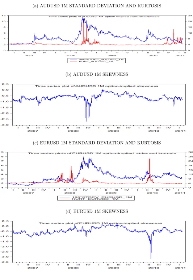
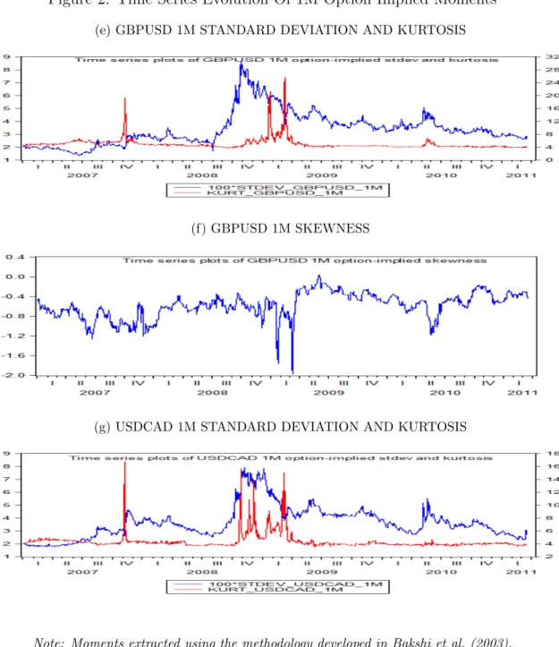
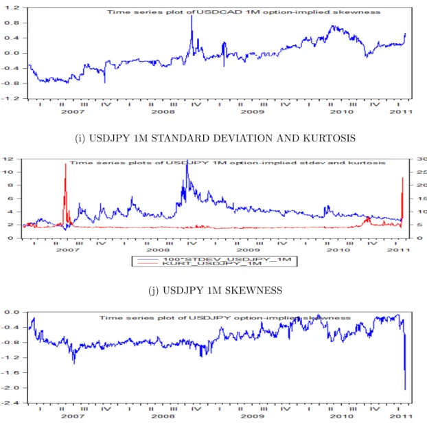
Summary statistics of the extracted moments are in table (2). 28 The summary statisticsshow that all the extracted moments are generally very persistent, with AR (1) coefficients as high as 0.99. Zivot and Andrews (1992) unit root tests, however, suggest that almost all the implied moments are stationary (with structural breaks in the means on dates around late 2008 and early 2009). For the rest of the analysis, we treat all variables as stationary.
Looking at the maximum and median for each series, as well as the time series plots, we see that there are a number of outliers, especially for the 9m and 12m moments. The time series plots in figure (2) show that these outliers are found mostly between late 2008 and early 2009.
INSERT TABLE (2) AND FIGURE (2) HERE
4.2
Can option-implied moments forecast FX excess returns?
4.2.1 Matched Frequency Analysis: Predictive ability of the volatility smile
We start by investigating whetherτ-period option-implied moments can explain the conditional mean of subsequent excess returns. Thus, for each currency pair i and tenor τ ,we estimate the following regression model by OLS:
fti,t+τ−Et(sti+τ) =γ0,τ +γ1,τstdev i,t+τ t +γ2,τskew i,t+τ t +γ3,τkurt i,t+τ t +ui,t+τ. (4.1)
Note that the LHS variable is ex-ante excess currency returns/forward bias. Under rational expressions, fti,t+τ −Et(sit+τ) is also equal to the risk premium. Gereben (2002) and Malz
28 Summary statistics for the option-implied moments of the other five currency pairs are similar, and can
be found in the online appendix. Time series plots forτ= 1W K,2M,3M,6M,9M and 12M are also in the online appendix.
(1997) also estimate regression specification (4.1) and interpret the results in light of the time-varying risk premia explanation of the UIP puzzle. Gereben (2002) argues that if the forward bias is due to time-varying risk premia, then variables that capture the nature of FX risk should be able to explain the dynamics of the forward bias. The option-implied moments on the RHS in regression equation 4.1), which capture perceived FX volatility, tail and crash risk should therefore be able to explain the forward bias. Malz (1997) also argues that statistical significance of the coefficient on skewtt+τ can be interpreted as providing support for the peso problem explanation of the UIP puzzle.
Going back to expression 4.1), we note thatEt(st+τ) is not observable. If we assume that
market participants have rational expectations, then Et(st+τ) and st+τ will only differ by a
forecast errorνt+1 that is uncorrelated with all variables that use information at timet, such
that
st+τ =Et(st+τ) +νt+1. (4.2)
Plugging equation (4.2) into equation (4.1) and rearranging gives us the following estimable regression equation: xrt+τ =γ0,τ +γ1,τstdev t+τ t +γ2,τskew t+τ t +γ3,τkurt t+τ t +t+τ (4.3)
where the error term t+τ = ut+τ + νt+τ and xrt+τ is ex-post excess returns defined in
expression (2.3).
To provide intuition regarding expected coefficient signs in the regression equation (4.3), we take the point view of a domestic investor who invests in domestic bonds using money borrowed from abroad. As shown in equation (2.3), such an investor benefits from higher domestic interest rates as well as appreciation of domestic currency. Let’s also assume that the home currency is riskier, such that our investor would demand higher excess returns for higher stdev and kurtosis in the exchange rate. If investors are averse to high variance and
kurtosis, they would require higher excess returns for holding bonds denominated in units of the riskier domestic and we would expect the coefficients on stdev and kurtosis to be both positive. We expect the skew coefficient to be positive for investor’s with preference for positive skewness. Such an investor will require higher compensation for an increase in skew, which represents a higher perceived likelihood of domestic currency depreciation.
Given the discussion in subsection (5.2), however, we note that pinning down the coefficient signs a priori is impossible without making further assumptions about the investor’s utility function or orthogonality of the moments. In our regression analysis, we therefore focus mainly on joint significance of the explanatory variables and model fit rather than on significance and signs of individual coefficients.
Sub-sample analyses suggest the presence of structural breaks in the matched-frequency regression relationships for the majority of currency pairs and tenors. We use the Bai and Perron (2003) structural break test to identify the date for the most prominent break29 and
estimate a modification of regression equation (4.3) that includes interactions with structural break indicator variable:
xrit+τ =γ0,τ +γ00,τD1i,τ +D1i,τ ∗γ1,τstdevi,tt +τ+D1i,τ ∗γ2,τskewi,tt +τ+D1i,τ∗
γ3,τkurti,tt +τ +γ4,τstdevti,t+τ +γ5,τskewti,t+τ +γ6,τkurtti,t+τ +it+τ.
(4.4)
where D1i,τ is an indicator variable that is zero before the break date and equal to one otherwise.
The matched-frequency results, shown in tables 3(a)-3(f), demonstrate a consistent ability of options-based measures of FX standard deviation, skewness and kurtosis-proxying to explain excess currency returns. The coefficients on the six non-intercept terms are always jointly significant, as shown by the low p-values for the Wald tests across currency pairs and across tenors. The adjustedR2s are also generally high across currency pairs and tenors, for
29We only focus on the major breaks, and therefore do not choose the number of breaks according to
example, ranging from 11% to 28% for 1M tenors .
We carry out a battery of robustness checks on the matched frequency results presented in table 3. First, we note that since we are using overlapping data, the R2s will be inflated.
30 To get an idea of the degree of R2 inflation and see if our results still change when we
use non-overlapping data, we re-run the regression (4.4) for 1M tenor using non-overlapping observations. We still use the same break date found from the regressions with overlapping data regressions, which are presented in table 3. The results of regressions with non-overlapping data regressions, shown in table (4a), suggest that the matched frequency results presented in table (3) are not being entirely driven by our use of overlapping data.
Results from sub-sample analysis and regressions using 10δ options (instead of 25δ) are presented in tables 4(b) and 4(c) respectively. Again, when we look at the adjusted R2s and
tests of joint significance of coefficients on the moments, we find that there are no major differences with the results presented in table (3).
Our final robustness check addresses the issue of outliers. The summary statistics of the extracted moments show some huge outliers. In the presence of outliers, ordinary least squares might give misleading results. For 3M tenor, we re-estimate the regressions specification (4.4) using robust least squares. Our estimation method addresses the presence of outliers in both the dependent variable and independent variables. Again, the main findings still hold, as can be seen in table table (4d).
INSERT TABLE (4) HERE
We digress from the bilateral analysis we have done so far in this section to investigate whether options-based measures of global volatility, skewness and kurtosis can explain the dynamics of bilateral excess returns. For the matched frequency global risk regressions, results of which are presented in 5(a), we extract the first three components from each of 3M 30For that reason, we do not interpret the higher R2s for 12m regressions as representing better fit at
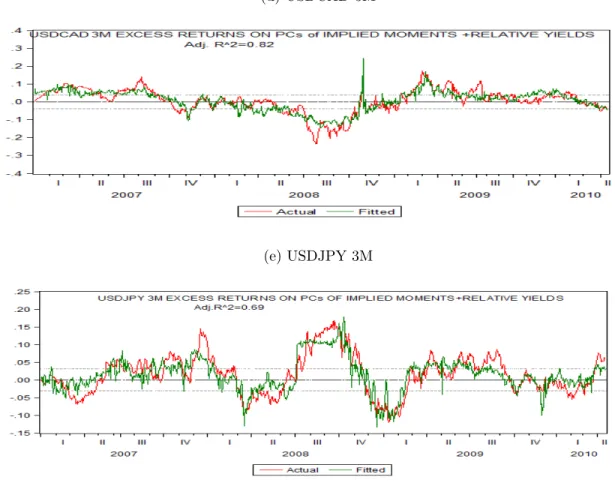
standard deviation, skewness and kurtosis across all currency pairs involving the USD. The coefficients on the pricincipal components are jointly significant, with adjusted R2s ranging from 14% to 26%. We then extend the global risk regression to incorporate term structure information by using principal components extracted from all currency pairs and from all tenors as regressors. The results from the term-structure of global risk regression, presented in table 5(b), show that information from the term structure of global risk adds further explanatory power, with adjusted R2s ranging from 16% to 40%.
INSERT TABLE (5 ) HERE
We next go beyond OLS regression, which models the conditional mean of the the dependent variable given the explanatory variables, by using quantile regression analysis (QR) to investigate the predictive ability of options-based FX risk measures for the entire distribution of ex-post excess currency returns. By modeling the entire distribution of the dependent variable, QR allows us to get a more complete picture of the predictive ability of the option-implied moments. QR also has a further advantage over OLS in that it is robust to outliers in the dependent variable and does not impose restrictive distributional assumptions on the error terms.
We estimate the following linear quantile regression model, modified to include one break:
Qxri (θ|.) = γ0,τ +γ1,τST DEVti,t+τ +γ2,τSKEWti,t+τ +γ3,τKU RTti,t+τ +i,t+τ, (4.5)
where Qxri (θ|.) is the θth quantile of excess returns given information available at time t.31 Matched-frequency quantile regression results for 3M tenor are shown in tables (6a)-(6f). We find that the coefficients on non-intercept terms are always jointly significant across quantiles for all currency pairs. Adjusted R2s are also consistently high, ranging from 16%
to 44% for AUDUSD and 10% to 26% for USDJPY for example. Another consistent pattern 31We estimate the quantile regression model using the same break dates obtained in the OLS analysis
across currency pairs and tenors is that option-implied moments have more predictive ability for lower and upper quantiles of excess returns than the middle quantiles.
INSERT TABLES (6a)- (6f)HERE
4.2.2 Can the term structure of implied moments explain FX excess returns?
The matched-frequency results presented in subsection (4.2.1)suggest that options-based measures of FX higher moment risks consistently explain subsequent bilateral excess returns. We now turn to studying the predictive ability of the term structure of options-implied moments for currency excess returns.
We first extend regression equation (4.3) by regressing 3M bilateral excess returns on 1M, 3M and 12M option-implied moments. That is, for each currency pair i, we estimate the following OLS regression:
xrti+3M =γ0,3M+X j γ1,τjstdevt+τj,i t + X j γ2,τjskewt+τj,i t + X j γ3,τjkurtt+τj,i t +it+3M, (4.6)
where j ∈ {1M,3M,12M}. Similar to the matched-frequency analysis in subsection (4.2.1), our final term structure regression model is a modification of (4.6) in which we include interactions with a structural break indicator variableD1. Regression results from specification (4.6) (with break ) are shown in columnBof table (7). Compared to the matched frequency results presented in columnA, we see a huge increase in the adjustedR2swith adjustedR2s
now ranging from 58% to 74% for the results from equation (4.6). In column Cof table (7) , we present condensed results of regressions that incorporate information from all tenors( not just 1M,3M and 12M) by using principal components extratced from all tenors.
xrti+3M =γ0,τ + 3 X j=1 γ2,jP CjstdevT ermi+ 3 X j=1 γ3,jP CjskewT ermi+ 3 X j=1 γ4,jP CjkurtT ermi+it+3M. (4.7)
In equation (4.7), P CjxxxxT ermi refers to the jth principal component extract from
the currency i term structure of option-implied moment xxxx. Results from estimation regression equation (4.7) are in column C of table (7).
Lastly, we extend the specification in (4.7) by adding information from the term structure of first moments as additional regressors:
xrti+3M =γ0,τ + 3 X j=1 γ1,jP CjmeanT ermi+ 3 X j=1 γ2,jP CjstdevT ermi+ 3 X j=1 γ3,jP CjskewT ermi+ 3 X j=1 γ4,jP CjkurtT ermi+it+3M. (4.8)
As we argued earlier, the term structure of first moments captures expectations of the dynamics of future macroeconomic fundamentals. We use the term structure of interest rate differentials to extract the principal components of the term structure of first moments of logSt+τ
St ) . As we noted in (3.1 ), under CIP, the forward premium f
t+τ
t −st,which is the
theoretical mean of the risk-neutral probability density of log
St+τ
St
is equal to the interest differentialiτ−i∗,τ.Using yield curve data to extract the term structure of first moments has
the advantage of allowing us to also use interest rate differentials for tenors not covered by our option price data. As with our previous regressions, we estimate a version of regression model (4.8) that includes interactions with a structural break indicator variable.
(D) of table (7). Actual vs fitted plots from this regression are shown in figures (3(a)-3(e)).
INSERT FIGURE (3) AND TABLE (7) HERE
The main finding from comparing columns C and D is that information from the term structure of first moments is not redundant. The adjusted R2s all show sizable increases,
and Wald tests for the null hypothesis that all coefficients on the first moment principal components are zero suggest the first moments are contributing additional explanatory power.
The main conclusion from analysis of the results presented in table (7) is that FX risks, captured by the higher order moments, and expectations, captured by the term structure of implied moments, have substantial explanatory power for ex-post excess currency returns.
4.3
Can option-implied moments forecast currency returns?
In subsection (4.3), we investigate the ability of options-based measures of higher moment risks and their term structures to explain currency returns ∆st+τ.
4.3.1 Can the volatility smile predict currency returns?
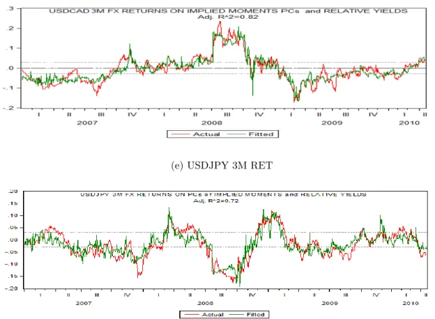
For each currency pair i, we start by estimating the standard UIP regression
sti+τ −sit =α+β(ftt+τi−sit) +it+τ (4.9) We focus on model fit and joint significance rather than testing whether the β coefficient is equal to 1. Fitted vs Actual plots of estimated regression (4.9) (with breaks) are shown in figures (4(a))-(4(e)), while condensed results can be found in column A of table (8).
estimating the following augmented UIP regression: sit+τ −sit=α+β1(fti,t+τ−st) +β2stdev i,t+τ t +β3skew i,t+τ t +β4kurt i,t+τ t +i,t+τ (4.10)
Equation (4.10) therefore augments the standard UIP equation (4.9) by studying the predictive ability of the 1st−4th moments of the distribution of logSt+τ
St
.
The condensed regressions results are shown in column B table (8) . The adjusted R2s for the matched-frequency augmented UIP regressions are consistently high and the higher order moments are always jointly significant.
INSERT TABLE (8) AND FIGURE (5) HERE
4.3.2 Can the term structure of implied moments predict currency returns?
We move on to studying whether the term structure of options-implied moments have predictive ability for subsequent FX returns. We start by estimating a term structure modification of the standard UIP equation (4.9) that uses information contained in the term structure of forward premia:
sit+τ −sit =γ0,τ +
3
X
j=1
γ1,jP CjmeanT erm+it+τ. (4.11)
Condensed results from regression specification (4.11) are presented in column C of table (8). Comparing columnsA and Cin table (8), we see that adding the whole term structure of forward premia significantly improves the UIP regression fit.
sit+3M −sit=γ0,τ + 3 X j=1 γ1,jP CjmeanT ermi+ 3 X j=1 γ2,jP CjstdevT ermi+ 3 X j=1 γ3,jP CjskewT ermi+ 3 X j=1 γ4,jP CjkurtT ermi+it+3M. (4.12)
Plots of actual versus fitted values from regression (4.12) are shown in figures (4) and the condensed regression results are in column D of table (8).
INSERT TABLE (8) AND FIGURE (4) HERE
Comparing columns C and D in table (8), we find that the term structure of 1st-4th moments adds a significant amount of explanatory power for exchange rate movements. The main conclusion from the results presented in table (8) is that higher order moments and expectations (captured through term structure dynamics) combine to explain subsequent exchange rate movements.
5
Further Interpretation and Discussion
5.1
Higher Moments Matter: Asset Pricing Derivation of UIP
Condition
32The fundamental asset pricing equation is given by
Et[Mt+τRt+τ] = 1, (5.1)
where Mt+τ is the pricing kernel and Rt+τ = StS+tτ is the gross return on an asset. Suppose
that assets can be denoted in domestic or foreign currency units. Under complete markets, 32The material in this subsection is from Backus et al. (2001)
the following relationship holds: Mt∗+τ Mt+τ = St+τ St (5.2)
where Mt∗+τ is the foreign pricing kernel. By taking logs and conditional expectations, expression (5.2) can be written as
Etst+τ −st=Et(logMt∗+τ)−Et(logMt+τ), (5.3)
where st =log(St).33 Applying pricing equation (5.1) to price a forward contract yields
Et[Mt+τ(Ftt+τ−St+τ)] = 0. (5.4)
Dividing equation (5.4) by St and using the result in expression in equation (5.2) gives the
expression for the forward premium:
ftt+τ −st =log(Et(Mt∗+τ))−log(Et(Mt+τ)) (5.5)
Applying the asset pricing equation (5.1) to price one-period domestic and foreign risk free bonds, we get expressions for the short rates: it =−log(Et(Mt+τ)) andi∗t =−log(Et(Mt∗+τ)).
Equation (5.5) and the expressions for short rates give us the CIP condition:
it−i∗t =log(Et(Mt∗+τ)−log(Et(Mt+τ) =ftt+τ−st. (5.6)
Finally, the expression for ex-ante currency excess returns or deviation from UIP condition 33Writing the returns in the form (5.3) also makes it clear why macroeconomic fundamentals such as
consumption growth are expected to explain currency excess returns. As pointed out by Backus et al. (2011), in macroeconomics, the pricing kernel is tied to macroeconomic quantities such as consumption growth. Expression (5.7) therefore suggests that the dynamics of FX returns should be explained by domestic and foreign macroeconomic fundamentals.
is therefore given by
ftt+τ−Etst+τ =it−i∗t−Etst+τ−st= (logEtMt∗+τ−EtlogMt∗+τ)−(logEtMt+τ−EtlogMt+τ).
(5.7) Under risk-neutrality the RHS of expression (5.7) is zero, and we get the forward unbiasedness condition ftt+τ = Etst+τ. Risk aversion is captured in the pricing kernel. Expression (5.7)
is therefore sometimes referred to as FX risk premium. Equation (5.7) makes it clear why the failure of the UIP condition is usually attributed to time-varying risk and expectational errors. Excess returns should theoretically depend on time-varying cross-country differences in risk, captured through the pricing kernels. This risk could include liquidity risk, business-cycle related risks, political risk, and liquidity risk. In macroeconomics, pricing kernel is linked to macroeconomic fundamentals such as consumption growth. Thus, expression (5.7) also suggests that currency excess returns should depend on differences in expected macroeconomic conditions. As we mentioned earlier, the difficulty faced by the literature is that standard proposed measures of risk do not appear to have strong correlation with excess returns.
Equation (5.7) is also insightful in showing how excess returns can potentially be explained by higher order moments. This can be seen clearly by expressing logEtMt+τ in terms of the
cumulants of the conditional distribution oflogMt+τ: logEtMt+τ =P ∞ j=1
κjt
j! ,whereκjtis the
jth cumulant of the conditional distribution of log(M
t+τ). Cumulants are closely related to
moments, and the expressions for the first four cumulants are : κ1t=µ1t, κ2t=µ2t, κ3t=µ3t
and κ4t = µ4t−3(µ2t)2, where µ1t is the conditional mean and µjt denotes the jth central
moment of the distribution of logEtMt+τ.
Equation (5.7) can therefore also be written in the form
ftt+τ −Etst+τ = ∞ X j=2 (κ∗j −κj) j! (5.8)
Equation (5.8) illustrates that currency excess returns will in general depend on the higher order moments of the distribution of the pricing kernel. Note that if we assume that pricing kernels are log-normally distributed, then expression (5.8) reduces to
ftt+τ −Etst+τ =
(µ∗2t−µ2t)
2 .
The preceding discussion yet again illustrates how distributional assumptions can potentially lead to a disregard for higher order moments which might crucial in empirical data.
5.2
Higher moments matter : asset allocation under higher order
moments
34We showed in subsection (2.2) that the assumptions of CARA utility and normality of returns reduce the investor’s problem to mean-variance optimization. However, if the distribution of portfolio returns is asymmetric, or the investor’s utility function is of a higher order than the quadratic, or the mean and variance do not completely determine the distribution of asset returns, then higher order moments and their signs must be taken into account in the portfolio asset allocation problem. In this subsection we present a framework for incorporating higher order moments into the asset allocation problem.
The objective in (2.4) can be intractable and it is usual to focus on approximation of (2.4) based on higher order moments. Jondeau et al. (2010) consider a Taylor’s series expansion of the utility function around expected utility up to the fourth order:
U(Wt+1) = U(EtWt+1) +U(1)(Wt+1)(Wt+1−EtWt+1) + 2!1U(2)(Wt+1)(Wt+1−EWt+1)2+ 1 3!U (3)(W t+1)(Wt+1−EtWt+1)3+4!1U(4)(Wt+1)(Wt+1−EtWt+1)4, (5.9) where Un(.) denotes the nth derivative of the utility function with respect to next period
wealth. Taking the conditional expectation of expression ( 5.9) yields Et[U(Wt+1)]≈U(EtWt+1) +U(1)(Wt+1)(Wt+1−EtWt+1) + 2!1U(2)(Wt+1)(Wt+1−EtWt+1)2+ 1 3!U (3)(W t+1)(Wt+1−EtWt+1)3+4!1U(4)(Wt+1)(Wt+1−EtWt+1)4. (5.10) Under the assumption that the investor’s utility function is CARA, expression (5.10) reduces to Et[U(Wt+1)]≈ −e−γµp h 1 + γ22σ2 p− γ3 6 s 3 p+ γ4 24k 4 p i . (5.11)
In equation (5.11),s3pandk4p are the skewness and kurtosis of portfolio return. It is clear from equation (5.11) that under CARA utility, investors prefer positive skewness and dislike high variance and high kurtosis. Optimal portfolio weights can then be obtained by maximizing expression (5.10) instead of the exact objective function shown in expression (2.4).
For CARA utility, the weight the investor puts on the higher order moments depends on the degree of risk aversion parameter γ. In more general settings, however, the weight on the nth moment depends on the nth derivative of the utility function, and the signs of sensitivities of utility function to changes in higher moments cannot be easily pinned down. If the moments are not orthogonal to each other, then the effect of utility of increasing one moment might not be straight forward. Scott and Horvath (1980) establish some general conditions for investor preference for skewness and kurtosis.
5.3
Higher Moments Matter: Higher order ICAPM
35 We start with the fundamental pricing equation,Et[Mt+τRit+τ] = 1 (5.12)